Localized LQR Optimal Control
Abstract
This paper introduces a receding horizon like control scheme for localizable distributed systems, in which the effect of each local disturbance is limited spatially and temporally. We characterize such systems by a set of linear equality constraints, and show that the resulting feasibility test can be solved in a localized and distributed way. We also show that the solution of the local feasibility tests can be used to synthesize a receding horizon like controller that achieves the desired closed loop response in a localized manner as well. Finally, we formulate the Localized LQR (LLQR) optimal control problem and derive an analytic solution for the optimal controller. Through a numerical example, we show that the LLQR optimal controller, with its constraints on locality, settling time, and communication delay, can achieve similar performance as an unconstrained optimal controller, but can be designed and implemented in a localized and distributed way.
I Introduction
Large scale systems pose many challenges to the control system designer: simple local controllers generated by heuristics cannot guarantee global performance (or at times even stability), whereas traditional centralized methods are neither scalable to compute, nor physically implementable. Specifically, a centralized controller requires computing with the global plant model for its synthesis (such a computation can quickly become intractable for large systems), and further necessitates that all measurements/control actions be collected/distributed instantaneously. In order to address the issues arising from communication constraints amongst sensors, actuators and controllers, the field of distributed optimal control has emerged. In particular, communication constraints often manifest themselves as subspace constraints in the optimal control problem, restricting the controller to respect specific delay and sparsity patterns.
It was soon realized, however, that the tractability of the distributed optimal control problem depends on how quickly information is shared between controllers, relative to the propagation of their control action through the plant. In particular when quadratic invariance (QI) [1, 2] holds, the distributed optimal control problem can be formulated in a convex manner – specifically, constraints in the Youla domain are then equivalent to constraints in the original “” domain, allowing the optimization to be written as a constrained model matching problem. With the identification of quadratic invariance as an appropriate means for convexifying the distributed optimal control problem, much progress has been made in finding finite dimensional reformulations of the optimization.
In the case of constraints induced by strongly connected communication graphs, computing the optimal controller has been reduced to solving a finite dimensional convex program in [3, 4] and [5]. In the case of sparsity constrained controllers, specific structures have been explicitly solved: including two-player [6, 7], triangular [8, 9], and poset-causal [10, 11] systems. It should also be noted that similar approaches to convex distributed optimal controller synthesis have been applied to spatially invariant systems satisfying a funnel causality property [12, 13].
Although the aforementioned results provide insight into the structure of the optimal controller, the applicability is highly limited to specific plant structures of moderate size. In particular, the distributed optimal controller is often as expensive to compute as its centralized counterpart, and even more difficult to implement. For example, if a plant has a strongly connected topology, (e.g. a chain), the QI condition requires that each controller share its measurements with the whole network – this becomes a limiting factor as systems scale to larger and larger size. Although several attempts have been made in the literature to find sparse controllers (which lead to tractable implementations), such as sparsity-promoting control [14, 15], and spatial truncation [16, 17], the synthesis procedure is still centralized. In this paper and our previous work [18], we advocate the importance of locality (i.e. sparsity in the controller and the closed-loop response) for the joint scalability of both computation and implementation.
The key observation in [18] was that a localized (and thus sparse and scalable) controller implementation does not mean that the information structure on controller (the transfer function from measurements to control actions) needs to be sparse. By allowing controllers to exchange both measurements and control actions, we showed that the controller implementation is localized if the system (with certain technical assumptions) is state feedback localizable. We characterize such systems in terms of the feasibility of a set of linear equations. These equations can be verified in a localized and distributed manner – further, the solution to these equations can be used to synthesize the controller achieving the desired closed loop response in a completely localized way. This offers a scalable design and implementation method that additionally achieves a localized closed loop performance.
This paper is an extension of the work in [18]. The primary contributions are that we (1) generalize the notion of state feedback localizability to non-scalar sub-systems, (2) propose a receding-horizon like control scheme that is numerically robust to computation errors, and (3) formulate the Localized LQR (LLQR) optimal control problem, and derive its analytic solution. In particular, we emphasize the fact that the LLQR optimal controller can be synthesized and implemented in a localized way.
The paper is structured as follows. Section II introduces the system model with spatio-temporal constraints and extends the notion of state feedback localizability to a general linear time invariant system. In Section III, we characterize localizable distributed systems by the feasibility of a set of linear equations, and propose a receding-horizon like controller implementation based on the solution of the local feasibility test. The robustness of the implementation is discussed in the same section. In Section IV, we formulate the LLQR optimal control problem and derive its analytic solution for both impulse and additive-white Gaussian noise (AWGN) disturbances. Section V compares the performance of our method to several different control schemes from centralized and distributed optimal control. Finally, Section VI ends with conclusions and offers some possible future research directions.
II Preliminaries
II-A System Model
Consider a discrete time distributed system with dynamics given by
| (1) |
where , and are stacked vectors of local state, control, and disturbances, respectively. The objective is to design a distributed dynamic state-feedback controller such that the transfer functions from to and to satisfy some spatio-temporal (locality) constraints. Throughout this paper, we use to denote the closed loop transfer function from to and the closed loop transfer function from to . The key idea in this paper is to force and to satisfy some spatio-temporal constraints, then show that the controller achieving the desired closed loop response can be synthesized and implemented by and . For any transfer function , we use to denote the -th spectral component of , i.e. . Thus in the time domain, the ordered set is the impulse response of the system.
II-B Spatio-Temporal Constraints
The spatio-temporal constraint on a transfer function can be specified by the sparsity pattern on each of its spectral component. Define the support operator , where iff , and otherwise. We define the entry-wise OR operation for two binary matrices . We say that if . The product with binary matrices of compatible dimension is defined by the rule
For a square binary matrix , we define for all positive integer , and . If is the support of the adjacency matrix of a graph, we define the distance from state to as
The sparsity pattern of a transfer function can be described by a set of binary matrices. Define constraint space by an ordered set of binary matrices . We say that a transfer function is in if and only if for all , which is denoted by . If for all , we say that is finite in time , and any transfer function in has a finite impulse response (FIR).
In order to impose locality constraints on the system, we introduce the notion of sparseness to measure how disturbances propagate through the plant.
Definition 1
We say that a real matrix is sparse if
A constraint space is sparse if and only if is sparse for all .11 1 For a large , it is possible that - this simply means that the “localized” region is the entire system.
Then, we define the following two sets to characterize the localized region for each state.
Specifically, contains all states with distance less than or equal to to -th state. Equivalently, it contains all the (possibly) nonzero elements in -th row of . contains all states with distance less than or equal to from -th state, which is equal to the set of all (possibly) nonzero elements in -th column of .
We can use to impose both sparsity and delay constraints. However, as the required communication delay constraints will depend on the implementation of the controller, we will discuss how these are constructed after we introduce the controller implementation in the next section.
II-C State Feedback Localizability
We now define localized FIR constraints and state feedback localizability for a system . Throughout this paper, we use to denote the constraint space for (the transfer function from to ) and the constraint space for (the transfer function from to ).
Definition 2
The constraint space pair is a localized FIR constraint for system if and only if
- 1.
and are finite in time .
- 2.
is sparse.
- 3.
is sparse.
The third condition of Definition 2 is key to extending our previous results [18] to non-scalar sub-systems.22 2 In this paper, each sub-system can contain several states and control signals. The and refer to a single state and a single control signal respectively, which are scalars. However, a scalar might affect several states at the same time, and a state might be affected by several control signals as well. Here, we not only want to localize the closed loop from to , but also want to achieve this by only using controllers in a localized region. For the scalar sub-system plant model that was considered in [18], the latter condition is automatically satisfied. For non-scalar sub-systems, we need to explicitly impose this constraint on the controller. State feedback localizability is then defined as follows.
Definition 3
Assume that is a localized FIR constraint for system . The system is state feedback -FIR localizable by if and only if there exists strictly proper transfer functions and such that
| (2) |
with .
Equation (2) is a relation that and must satisfy when the system dynamics are given by (1). To see this, apply an impulse disturbance at state in (1), i.e. . The closed loop response of and in (1) is by definition the -th column of and respectively. Therefore, a valid closed loop transfer function pair must satisfy (2). In addition, being a localized FIR constraints implies that and for all , meaning that and are both FIR as well.
Definition 3 has an intuitive interpretation in the time domain. For a -FIR localizable system, a local disturbance only affects with , and the effect will be eliminated in time . Furthermore, we only need to activate the local controllers for in order to localize the affected region. As illustrated in Figure 1, the affected region of is confined to the right section in the space-time diagram, which we call the forward space-time region for .

Imposing space-time constraints on the closed loop has the added benefit that the controller can then be implemented in a localized manner. Assume that the disturbance can be perfectly estimated. Then, each local controller only needs to collect the estimated disturbances from a backward space-time region as shown in Figure 1. Hence we can impose communication delay constraints for information collection through this region by ensuring that the backward space-time region is contained within an allowable region. We will discuss the relations between the closed loop (forward region) and controller implementation (backward region) in more detail in the next section.
III Feasibility Characterization and Controller Implementation
In this section, we give a feasibility test that characterizes localizable distributed systems, and that can be performed in a localized manner. We then show how a receding-horizon like controller can be synthesized based on the solution of the local feasibility test. Finally, we show that this implementation is robust with respect to computation error, and therefore especially useful for use with open-loop unstable systems.
III-A Local Feasibility Characterization
Let be a localized FIR constraint for . To check whether is -FIR localizable by , we can simply rewrite (2) and formulate the global feasibility test as
| (3) |
The feasibility of (3) can be verified in a localized manner by selecting each column of and . The fact that is a localized FIR constraint enables us to further reduce the dimension of each local feasibly test. In particular, let , , and apply an impulse disturbance to (1). As is a localized FIR constraint, we know that the nonzero states in , , and are all contained in , motivating the definition of -reduced state and control vectors [18].
Definition 4
The -reduced state vector of consists of all local state with and is denoted by . Similarly, the -reduced control vector of consists of all local control with and is denoted by .
We can then define the -reduced plant model by selecting submatrices of consisting of the columns and rows associated with and . The -reduced constraint space can be defined in a similar way. In addition, we denote by the new location of the source of disturbance within the reduced state . In this case, (1) can be simplified to
| (4) |
We can express (4) in the form of (3), and formulate the -th local feasibility test as
| (5) |
where and are the -th column of and respectively.
To prove the equivalence between the global feasibility test and local feasibility test, we define the embedding linear operators on and on , which simply add appropriate zero padding such that and , where and are the -th column of and respectively. In particular, we have that . The equivalence between local and global feasibility test is given by the following theorem.
Theorem 1
Proof:
See Appendix. ∎
Remark 1 (Robustness to local changes)
Equation (5) indicates that the solution only depends on the local plant model . Therefore, when a plant model changes locally, we only need to resolve some of the local feasibility tests to check whether it is still localizable.
For each local feasibility test (5), we can explicitly express the state trajectory over the horizon as a function of control input as
| (6) |
where
with , and and the stacked sparsity constraints that can be derived directly from (5). The form of (6) is the same as the traditional way to check controllability of a system. We can then interpret state feedback localizability as a generalization of controllability within a space-time region.
In the next section, we will show that the global LQR problem for localizable system can be decomposed into several local optimization problems with (6) being the constraint on local plant dynamics for each local optimization problem. However, we will first show that any state feedback localizable system admits a localized controller implementation.
III-B Controller Synthesis and Implementation
After solving (5) for all , we can reconstruct the solution of (3) by applying Theorem 1. For each time step , the controller can be implemented via
| (7) | |||||
| (8) | |||||
| (9) |
At each time step, every controller (i) collects estimated disturbances from its backward space-time region, (ii) computes its control strategy and reference trajectory based on the collected estimated disturbances by (7)-(8), (iii) applies the control action and measures its own state, and (iv) computes its own estimated disturbance by (9) and broadcasts it out to its forward space-time region. This general strategy, as implemented at a single node, is illustrated in Figure 1.
We can now formally discuss the relation between the backward space-time region and forward space-time region in Figure 1. In particular, the backward space-time region is defined by the sparsity pattern of the rows of and , and the forward space-time region by the sparsity pattern of the columns of and .
For example, from (7) and the sparsity pattern of the -th row of , each local controller only needs to collect , for , with , to generate its control action. Similarly, to generate , we only need to collect , for .
For the forward space-time region, we need to show that the distributed controller (7) - (9) indeed yields the desired closed loop responses and . The key is to show that is a perfect estimate of the disturbance . Substituting (1) into (9), we get
| (10) | |||||
Substituting (7) and (8) into (10) and using the identity for with , we can derive . As is a perfect estimate of , the transfer functions from to and to are indeed and . Therefore, a local disturbance only affects with , and we only need to activate the local controls for to localize the effect of the disturbance.
The localized synthesis procedure follows from a combination of the sparsity patterns of the rows and columns of and . Focussing on , we see that to synthesize the reference trajectory generator for , we need to collect the solutions of the -th local feasibility tests, for . To solve the -th local feasibility test, we need to know the plant model associated with . Combining these two arguments, we can synthesize (7) - (9) via a local feasibility test following by a local update procedure. A complete localized synthesis procedure for scalar sub-systems can be found in Algorithm 1 of [18].
Finally, we can examine the communication delay constraints in the controller implementation. For simplicity, we assume that each sensor computes its own reference trajectory (8) and that the sensing delay is the same at every state. In order not to degrade the system’s performance, the reference trajectory must be generated before the state measurement is obtained. To ensure this property, we require the communication delay between any two states within the localized region to be less than the plant propagation delay. For example, if the constraint space satisfies
for all , a simple proof by induction shows that all local reference trajectories can be generated before they are needed. In this case, can be calculated once is available. Then, the delay constraint on is just the usual information sharing constraint from to , but delayed by one time step since is calculated from .
III-C Sensitivity Analysis
An advantage of using this receding-horizon like control scheme (7) - (9) is its numerical robustness. Assume some computation error in the feasibility test, that is, for some perturbation matrices , . From (10), we can derive
| (11) |
If the norm of each is small enough, then will be bounded and hence so will and . Notice that when a system cannot be exactly localized, we can use (11) to bound the performance degradation as well.
Assume now that there is only one disturbance at time . If we neglect the higher order terms for , we have that
| (12) |
for – through a more detailed, but standard, analysis, one can use the small gain theorem to quantify the maximum allowable for stability. On the other hand, if we do not use (7) - (9), and estimate directly from the measured state and control action instead as
| (13) |
then the computation error will accumulate over time for unstable . Using (13) for the same disturbance , we will have
| (14) |
If the original system is unstable, then would grow unbounded for large for any non-zero .
The robustness of the receding-horizon like implementation can also be interpreted in the frequency domain. After solving the feasibility test, we obtain a pair of localized transfer functions such that and . A naive approach to implementing the controller is via , which results in (14). This is ill-conditioned since the controller is attempting to cancel the unstable open-loop dynamics. Instead, the frequency domain interpretation of equations (7) - (9) are
We actually use another feedback loop to compute based on without explicitly inverting the plant. Nevertheless, we need to ensure that the communication between controllers is fast enough such that the delay introduced by this extra feedback loop does not degrade the system performance and maintains localizability.
IV Localized LQR Optimal Control
IV-A Optimal Control Problem Formulation
The localized optimal control problem can be formulated as the following affinely constrained convex program:
| subject to | (3) | (15) |
for some convex function . Localizability is determined by the feasibility of this optimization problem. Note that as the closed loop system is constrained to be FIR, traditionally infinite dimensional objectives and constraints, such as those present in optimal control, trivially admit a finite dimensional representation.
IV-B LLQR Optimal Controller for Impulse Disturbances
For a general objective function in (15), the optimization cannot necessarily be solved in a localized way. However, when the cost function is chosen to be LQR, leading to a LLQR optimal control problem, (15) can be decomposed in exactly the same way as the local feasibility test. Thus, the optimal LLQR controller can be synthesized based on local optimizations followed by local update procedures, which are similar in spirit to Algorithm 1 in [18].
Given a positive semi-definite matrix and a positive definite matrix , we define the LLQR problem as
| subject to | (16) |
Letting be the number of states, the objective in (16) can be written as
| (17) |
As trace is invariant under cyclic permutation, we can write (17) as
Using Theorem 1, each and can be solved for via the -th local feasibility test. Thus, we can decompose the full objective in (16) into the sum of local objectives and formulate the reduced LLQR problem for the reduced trajectory and as
| subject to | (6) | (18) |
where and are submatrices of consisting of the columns and rows associated with and . To lighten notational burden, we drop all subscripts and write (6) as , , and . In addition, we define as the augmented block diagonal matrix with along the block diagonal. The objective in (18) can therefore be written in a single term . The analytic solution of (18) can be derived as follows.
Noting that is an affine constraint that forces some of the elements of to be zero, we can eliminate this constraint by selecting the appropriate columns of matrix to form a reduced matrix such that
where is the reduced unconstrained control signal.
Similarly, we can impose the constraint by selecting the corresponding rows on and . Specifically, we define matrices and by selecting the rows of and according to the positions of the zero entries in , and the rows of and according to the positions of the nonzero entries in . The equation is then separated into two parts:
| (19) | |||||
| (20) |
where (19) corresponds to the sparsity constraints imposed by , and (20) enforces that the non-zero states satisfy the dynamics.
We define the submatrices of associated with the support of and respectively. Then, (18) becomes
| subject to (19) and (20) | (21) |
Substituting (20) into the objective function, we have
| subject to | (22) |
If this problem is feasible, then we can solve the quadratic optimization via its optimality conditions
| (23) |
In summary, the reduced LLQR problem is subject to the constraint in (22), and has the optimal solution given by (23), implying that the LLQR optimal controller can be synthesized by solving a set of linear equations. Although the problem size of (23) is proportional to time , it is independent to the size of the global plant model since we only need to know the local plant model for each -th LLQR feasibility test. This property is especially favorable for large scale distributed systems. Future work will look to find a dynamic programming based solution to remove this linear scaling with .
IV-C LLQR Optimal Controller for AWGN Disturbances
In this subsection, we show that the controller synthesized by (16) is also mean square error optimal with respect to AWGN disturbances, i.e. we assume that and for all . The objective is to minimize
| (24) |
for . For , we have . As is determined by for , and are uncorrelated. Therefore,
Notice that . As expectation distributes over the trace sum, we can write
| (25) |
Substituting (8) into , we can then derive that
| (26) |
Summing (25) and (26) gives the first term in the objective in (16). Similarly, we can show that for ,
Therefore, the objective in (24) will converge to the objective in (16) as , implying that the controller synthesized for the impulse disturbances is also optimal in expectation for AWGN disturbances.
In general, imposing FIR or locality constraints degrades the transient performance of the controller, so our controller is not optimal. However, we will see in the next section via a numerical example that by choosing appropriate , the difference becomes negligible.
V Performance Comparison
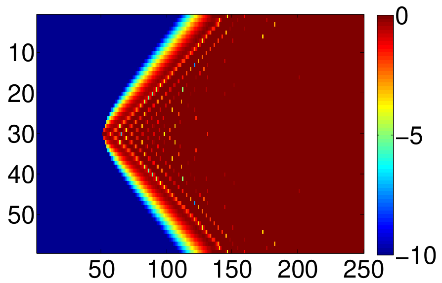


In this section, we synthesize our LLQR optimal controller for a specific plant, and compare the performance with different classes of optimal controllers from [3]. In particular, we consider the centralized, delayed centralized and optimal distributed (with quadratically invariant (QI) information sharing constraints) controllers.
The plant model is given by , where is a tridiagonal matrix with dimension given by
The instability of the plant is quantified by the spectral radius of , which is . is a matrix with the -th and -th entries being and zero elsewhere, . Even though our method can be applied to an arbitrary plant topology, we use this simple plant model as it leads to easily visualized representations of the aforementioned space-time regions.
For the LLQR controller, we choose . For all controllers with communication delay constraints, we assume that the communication network has the same topology as the physical network, but the speed is times faster than the speed at which dynamics propagate through the plant. The spatio-temporal constraint for the LLQR controller is given by
| (27) |
We then solve (16) with and set to identity.
We illustrate the difference between the different control schemes by plotting the space-time evolution of a single disturbance hitting the middle state. A concrete realization of a localized forward space-time region is in Figures 2(h) and 2(i): the effect of the disturbance is limited in both state and control action in time and space.
Next, we calculate the optimal value for each controller and summarize the results in Table I. The objective is normalized with respect to that of the centralized controller. Clearly, LLQR controller can achieve similar performance to that of the centralized one. Numerical evidence seems to suggest that this property holds for most plants that are localizable. For an ideal controller, the closed loop response decays exponentially in both time and space, as indicated by Figures 2(b) and 2(c). Therefore, it is generally possible to find a favorable to synthesize the LLQR controller such that the closed loop transient response does not degrade much – this is akin to the insight in [13] used to localize the implementation of funnel-causal systems.
In summary, our result demonstrates that the LLQR optimal controller can be synthesized and implemented in a localized manner, but can achieve transient response close to that of an unconstrained optimal controller.
| Ideal | Delayed | Distributed | LLQR | |
| Comm Speed | Inf | 1.5 | 1.5 | 1.5 |
| Control Time | Inf | Inf | Inf | 29 |
| Locality | Max(58) | Max(58) | Max(58) | 9 |
| Objective | 1 | 126.7882 | 1.1061 | 1.1142 |
VI Conclusion
In this paper, we introduced the notion of state feedback localizability through a feasibility test consisting of a set of linear equations. From the solution of the local feasibility tests, we synthesized a receding horizon like controller achieving a localized closed loop. We showed that this implementation is localized and robust with respect to computation error, and is particularly well suited to unstable plants. The Localized LQR optimal control problem was formulated, and its analytic solution was derived. Through numerical simulation, we further showed that the LLQR optimal controller achieves similar transient performance to that of an unconstrained optimal controller.
In the future, we will look to extend these results to output feedback, and to more rigorously analyze the robustness of our scheme.
APPENDIX
The following lemma is useful to prove Theorem 1. We assume that is a localized FIR constraint for .
Lemma 1
Suppose that and . Then
| (28) |
| (29) |
Proof:
We only prove equality (28), as (29) follows from a nearly identical argument. implies that the support of is contained within . Let be a state such that and a state such that : then . Let be a matrix of the same dimension as , but only have one (possibly) non-zero entry at -th location. Clearly, . Therefore, setting the -entry of to zero does not change the value of the RHS of (28).
Similarly, let be a state such that . Letting be a matrix of the same dimension as , but with only one (possibly) non-zero entry at -th location, we then also have for all . Thus setting the -entry of to zero does not change the value of the RHS of (28).
Repeatedly applying this argument, we can explicitly set all the elements in the -th row/column of to zero, without changing the value of the RHS of (28) – clearly this implies that the desired equality indeed holds. ∎
Now, we can prove Theorem 1.
Proof:
Assume that is a feasible solution for (5). Applying the operator to both sides of (4) and using Lemma 29, it is straightforward to verify that satisfy (1). In addition, and , so the global feasibility test is feasible.
To show the opposite direction, assume that is a solution to the global feasibility test. It suffices to show that satisfy the same sparsity constraints as . This directly follows from the fact that is a localized FIR constraint for . ∎
References
- [1] M. Rotkowitz and S. Lall, “A characterization of convex problems in decentralized control,” Automatic Control, IEEE Transactions on, vol. 51, no. 2, pp. 274–286, 2006.
- [2] M. Rotkowitz, R. Cogill, and S. Lall, “Convexity of optimal control over networks with delays and arbitrary topology,” Int. J. Syst., Control Commun., vol. 2, no. 1/2/3, pp. 30–54, Jan. 2010. [Online]. Available: http://dx.doi.org/10.1504/IJSCC.2010.031157
- [3] A. Lamperski and J. C. Doyle, “Output feedback model matching for decentralized systems with delays,” in 2013 IEEE American Control Conference (ACC), June 2013.
- [4] ——, “The control problem for decentralized systems with delays,” arXiv preprint arXiv:1312.7724v2, 2014.
- [5] N. Matni, “Distributed control subject to delays satisfying an norm bound,” in 2014 53th IEEE Conference on Decision and Control (CDC), To appear, 2014. [Online]. Available: http://arxiv.org/pdf/1402.1559.pdf
- [6] L. Lessard and S. Lall, “Optimal controller synthesis for the decentralized two-player problem with output feedback,” in 2012 IEEE American Control Conference (ACC), June 2012.
- [7] L. Lessard, “State-space solution to a minimum-entropy -optimal control problem with a nested information constraint,” arXiv preprint arXiv:1403.5020v2, 2014.
- [8] C. W. Scherer, “Structured -optimal control for nested interconnections: A state-space solution,” arXiv preprint arXiv:1305.1746v3, 2013.
- [9] T. Tanaka and P. A. Parrilo, “Optimal output feedback architecture for triangular LQG problems,” in 2014 IEEE American Control Conference (ACC), June 2014.
- [10] P. Shah and P. A. Parrilo, “-optimal decentralized control over posets: A state space solution for state-feedback,” in Decision and Control (CDC), 2010 49th IEEE Conference on, 2010.
- [11] ——, “An optimal controller architecture for poset-causal systems,” in 2011 50th IEEE Conference on Decision and Control and European Control Conference (CDC-ECC),, 2011.
- [12] B. Bamieh, F. Paganini, and M. A. Dahleh, “Distributed control of spatially invariant systems,” Automatic Control, IEEE Transactions on, vol. 47, no. 7, pp. 1091–1107, 2002.
- [13] B. Bamieh and P. G. Voulgaris, “A convex characterization of distributed control problems in spatially invariant systems with communication constraints,” Systems & Control Letters, vol. 54, no. 6, pp. 575–583, 2005.
- [14] M. Fardad, F. Lin, and M. R. Jovanovic, “Sparsity-promoting optimal control for a class of distributed systems,” in 2011 IEEE American Control Conference (ACC), June 2011.
- [15] F. Lin, M. Fardad, and M. R. Jovanovic, “Design of optimal sparse feedback gains via the alternating direction method of multipliers,” Automatic Control, IEEE Transactions on, vol. 58, no. 9, pp. 2426–2431, 2013.
- [16] N. Motee and A. Jadbabaie, “Approximation methods and spatial interpolation in distributed control systems,” in 2009 IEEE American Control Conference (ACC), June 2009.
- [17] N. Motee and Q. Sun, “Sparsity measures for spatially decaying systems,” arXiv preprint arXiv:1402.4148v1, 2014.
- [18] Y.-S. Wang, N. Matni, S. You, and J. C. Doyle, “Localized distributed state feedback control with communication delays,” in 2014 IEEE American Control Conference (ACC), June 2014.