Triple- and Quadruple-Gluon Azimuthal Correlations from Glasma and Higher-Dimensional Ridges

In nucleus-nucleus collisions, ridges occur in the di-hadron correlations as structures that are elongated in pseudorapidity difference $\Delta\eta=\eta_{1}-\eta_{2}$, and peak on the near $\Delta\phi\sim 0$ and away sides $\Delta\phi\sim\pi$, where $\Delta\phi_{1}-\phi_{2}$ is the azimuthal angle difference between hadron pairs. The origin of these correlations have long been ascribed to the interplay between these two effects: The rapidity correlations between the gluons that are produced from the same longitudinal color flux tube and the radially outward collective flow due to quark gluon plasma giving rise to the azimuthal collimation and anti-collimation of hadron pairs in the near and away sides, respectively. Historically, the appearance of collective flow as the prime indicative of quark gluon plasma have been thought to be specific to nucleus-nucleus collisions, and ridges had not been observed experimentally, nor had they been predicted by event generators particularly for p–p collisions until recently.

This established idea [1] has been challenged when the CMS collaboration at LHC announced the discovery of the ridge in high-multiplicity p–p collisions at ${\sqrt{s}=7\;\mathrm{TeV}}$ [2, 3, 4]. Soon after, this was followed by the discovery of the ridge in p–Pb collisions at ${\sqrt{s}=5.02\;\mathrm{TeV}}$ [5, 6, 7, 8, 9, 10, 11]. This puzzling situation gave rise to the question whether quark gluon plasma has been created even in small systems such as p–p and p–Pb. Relativistic hydrodynamics that employ the collective flow idea has been applied to these small systems, and interesting results have been obtained for p–Pb [12, 5, 13, 14, 15, 16, 17] and p–p collisions [18].

Another approach to explain the ridges in p–p and p–Pb collisions comes from saturation physics, and particularly its implementation within the glasma framework. Glasma (“glassy plasma”) refers to the flux tubes of classical $SU(3)$ color fields which result from high density color charge in the projectile and target at small-$x$. High gluon density in a nucleon or nucleus also gives rise to the emergence of the semi-hard saturation scale $Q_{\mathrm{s}}$, which itself makes diagrammatic approach feasible. Recently, the double-gluon glasma diagrams have been combined with the double-gluon BFKL diagrams, which are important at small-$x$ regardless of the gluon saturation. The variation of the ridge signal in the data for various momentum windows and multiplicity classes (“systematics”) in p–p and p–Pb collisions has been reproduced successfully without resorting to any collective flow in hydrodynamical sense [19, 20, 21, 22, 23, 24].

All these recent developments invite further studies that can possibly distinguish the underlying mechanism of the ridges. By deriving the triple- and quadruple-gluon azimuthal correlation functions in the gluon saturation regime we aim to take the first step towards this direction. For quantitative predictions on the triple- or quadruple-hadron spectra, one must convolve these gluon correlation functions with fragmentation functions, which will be performed in a separate study. Triple- and quadruple-hadron spectra can also be computed from hydrodynamics simulations, and data on these higher order hadron correlations can be another ground for testing the two frameworks; glasma and hydrodynamics.

Currently both glasma and hydrodynamics are seen as competing approaches (see the discussion in Ref. [25]). However, even in the case that hydrodynamics as a coarse grained model captures the liquid behavior of possible quark gluon plasma in p–p and p–Pb collisions, it would be desired to know how collectivity arises on a more fundamental level. Since successful applications of hydrodynamics to water do not preclude the existence of more fundamental van der Waals forces, we can ask what the van der Waals forces of quark gluon plasma might be.

In perturbative QCD, hadronic and nuclear collisions are understood as interaction of two partons from the projectile and target, which themselves are modeled in terms of parton distribution functions. One then adds radiative corrections to this picture by resumming logarithms of virtuality $Q^{2}$, Bjorken-$x$ or both simultaneously. Depending on the kinematic regime of the events, one of the resummation schemes such as DGLAP, BFKL, Double Logarithmic Approximation is followed. However, the conventional parton distribution functions constructed this way do not include gluon saturation. The two main effects of gluon saturation are slowdown of the unbounded growing of the gluon density, and the non-kinematical, nontrivial correlations between produced gluons depending on their transverse momenta and rapidities. In this work, we use unintegrated gluon distributions (UGD) from the running coupling Balitsky-Kovchegov (rcBK) evolution equation; these UGDs include gluon saturation effects. The non-kinematical correlation effect is captured by glasma diagrams which we shall calculate to triple- and quadrupole-gluon order. Any final quantitative study should combine gluon productions from both perturbative QCD and glasma diagrams.

This paper is organized in a way that first the well-known single- and double-gluon azimuthal cumulants are reviewed. By this, we aim to clarify the confusion in the literature regarding the prefactors, and in the mean time we will be showing the steps of glasma calculations over the relatively easier cases of the single- and double-gluon inclusive distributions. Then, we move to the derivation of the triple- and quadruple-gluon inclusive distributions. Finally we show the results of our numerical calculations where we use the UGDs obtained from the rcBK equation. We leave the quantitative predictions on the triple- and quadruple-hadron azimuthal correlations for another study; this requires convolving the triple- and quadruple-gluon correlations with fragmentation functions to attain final hadron spectra. However, our results based on gluons and how they change with the variance of transverse momentum and rapidity as well as the number of participants as presented in the last section can be seen as qualitative predictions for the future measurement on triple- and quadrupole-hadron correlations at LHC for p–p and p–Pb collisions.

In this section we first give an overview of the single- and double-gluon inclusive distribution functions from glasma. The purpose of this section is introducing the main steps of diagram calculation in glasma as well as determining the correct prefactors of the azimuthal cumulants which is mostly unsettled in the literature (See Appendix B).

We start with the single-gluon inclusive distribution function. The rate for a single gluon in the leading order is given by [26]

where the gluon production amplitude is

Here $p=(E,\boldsymbol{p})$, $A^{a,\mu}(p)$ is the classical gluon field with color index $a$, and it satisfies the classical Yang-Mills equation with the sources of color charge density $\rho^{a}_{1}(\boldsymbol{x}_{\perp})$ and $\rho^{a}_{2}(\boldsymbol{x}^{\prime}_{\perp})$ of the projectile and target. The polarization vector of the produced gluon with polarization $\lambda$ is denoted by $\epsilon_{\mu}^{(\lambda)}$. By transforming the Lorentz invariant phase space factor as ${d^{3}\boldsymbol{p}/E_{p}\longrightarrow d^{2}\boldsymbol{p}_{\perp}dy_{p}}$, one can write the leading order single-gluon inclusive distribution as

Classical gauge fields due to the color charge density of the target and projectile in the leading order in powers of $\tilde{\rho}^{a}_{1,2}/\boldsymbol{k}^{2}_{\perp}$ can be written as follows¹¹ 1 Equation (4) appeared with an extra factor of $1/2$ in Ref. [1]; however, this mistake has been corrected in a footnote in Ref. [27]. [28, 26, 29, 30]

where $f^{abc}$ is the structure constant of the gauge group, $g$ is the gauge coupling and $L^{\mu}$ is the Lipatov vertex whose components in the light-cone coordinates are given by

By substituting Eq. (4) into Eq. (3) and making the replacement $\sum_{\lambda}\epsilon_{\mu}^{*(\lambda)}\epsilon_{\nu}^{(\lambda)}\rightarrow-g_{\mu\nu}$, the single-gluon inclusive distribution can be written as

The glasma diagram corresponding to the single gluon production is shown in Fig. 1.

In a given collision $\tilde{\rho}^{a}_{1}$ and $\tilde{\rho}^{a}_{2}$ are not known; so for any quantity one proceeds by taking the average of it over the ensemble containing all possible color charge configurations of the projectile and target,

Here the weight function $W[\rho_{1,2}]$ evolves with JIMWLK renormalization group equation [31, 32, 33, 34, 35, 36, 37] and it already includes resummations in powers of $\alpha_{\mathrm{s}}\ln(1/x_{1,2})$, where $x_{1,2}$ are the Bjorken-$x$ values of the partons from the projectile and target [28, 38, 39, 40]. In the approximation of the local (white noise) Gaussian fluctuations of the McLerran-Venugopalan model [1, 41, *McLerran:1993ka, *McLerran:1994vd, 44, 45], the average of multiplication of many charge densities as in Eq. (3) can be written in terms of the two-point correlation function

where $\mu^{2}(y_{p},\boldsymbol{k}_{\perp})$ is the Fourier transform of the color charge squared per unit transverse area, and $y_{p}$ is the momentum rapidity of the produced gluon. Here only the densities from the same nucleon or nucleus are correlated. After averaging Eq. (8) over all possible color charge configurations, and by using Eq. (10) and ${f_{abc}f_{abc}=N_{c}(N_{c}^{2}-1)}$, one arrives at

where $S_{\perp}$ is the transverse area of the overlap between the target and projectile, and it results from the replacement

The unintegrated gluon distribution per unit transverse area (UGD) is defined as [28]

By using Eq. (13) and $L^{\mu}(p,\boldsymbol{k}_{\perp})L_{\mu}(p,\boldsymbol{k}_{\perp})=-4\boldsymbol{k}_{\perp}^{2}(\boldsymbol{p}_{\perp}-\boldsymbol{k}_{\perp})^{2}/\boldsymbol{p}_{\perp}^{2}$, Eq. (11) becomes²² 2 Our result here matches with the one in Ref. [28].

where we used the compact notation $\Phi_{1,p}(\boldsymbol{k}_{\perp})\equiv\Phi_{A_{1}}(y_{p},\boldsymbol{k}_{\perp})$.

We now turn to the calculation of the double-gluon inclusive distribution from classical color fields in the leading logarithmic order. We start with

where

After using Eq. (4), we end up with

This leads to 9 distinct diagrams in total as there are three different contractions for each of the projectile and target. In Fig. 2 we show one of the 8 connected diagrams along with the disconnected diagram. Out of the 8 connected diagrams, we shall only consider the “rainbow” diagrams as in Ref. [28]; there are 4 such diagrams. Rainbow diagrams are the leading diagrams where dimers with the same momentum index are contracted among each other either on the upper or lower part of a given diagram, as in the connected diagram in Fig. 2. The tools for contractions and diagram calculation are explained in Appendix A.

The disconnected diagram in Fig. 2 can be seen as two separate single-gluon diagrams as shown in Fig. 1. A more useful quantity is the connected double-gluon correlation function which is defined as

where the subscript “LLog” will be suppressed henceforth. The disconnected contribution that is contained in the first term in Eq. (18), which contains 4 connected and 1 disconnected diagram, is subtracted by the second term. Hence calculating only the 4 connected diagrams will directly yield second cumulant $C_{2}(\boldsymbol{p},\boldsymbol{q})$.

In the calculation of $C_{2}(\boldsymbol{p},\boldsymbol{q})$ one should consider not only the contractions between the dimers across the cut line, but also contractions among the dimers on the same side of the cut line. Hence, all of the correlators below are needed

We use Eq. (19) when two dimers from opposite sides are contracted, and Eqs. (20) and (21) when two dimers from the same side are contracted. The rapidity index of $\mu^{2}$ in Eqs. (19), (20) and (21) will be determined as follows. We choose a convention that $y_{p}$ is closer to the rapidity of the projectile and $y_{q}$ is closer to the rapidity of the target. Hence, when contracting two charge densities, one connected to the gluon with momentum $\boldsymbol{p}$ and the other to the gluon with momentum $\boldsymbol{q}$ (see Fig. 2), one should take $y_{p}$ if the charge densities have nucleus index $1$ (projectile), and $y_{q}$ is the they have nucleus index $2$ (target)

This convention is independent of whether the $\tilde{\rho}$’s are the starred ones or not.

The rest of the calculation is similar to that of the single gluon except that here we also use $f^{abc}f^{abd}=N_{c}\delta^{cd}$. The double-gluon inclusive distribution have the form³³ 3 The mistake in the prefactor in Ref. [28] has been corrected in Ref. [20] where “$\int_{\boldsymbol{k}_{\perp}}$” means “$\int d^{2}\boldsymbol{k}_{\perp}$” without a factor of $1/(2\pi)^{2}$. As for Eq. (12) in Ref. [27], it does not reproduce correctly neither the prefactor of Eq. (24) here nor the momentum dependence of the UGDs in Eq. (27).

where

The double-gluon correlation function $C_{2}(\boldsymbol{p},\boldsymbol{q})$ in Eq. (24) has recently been used to explain the ridges seen in the di-hadron correlations in p–p ($\sqrt{s}=7\;\mathrm{TeV}$) and p–Pb ($\sqrt{s_{NN}}=5.02\;\mathrm{TeV}$) collisions at LHC [19, 20, 21, 22, 23, 24].

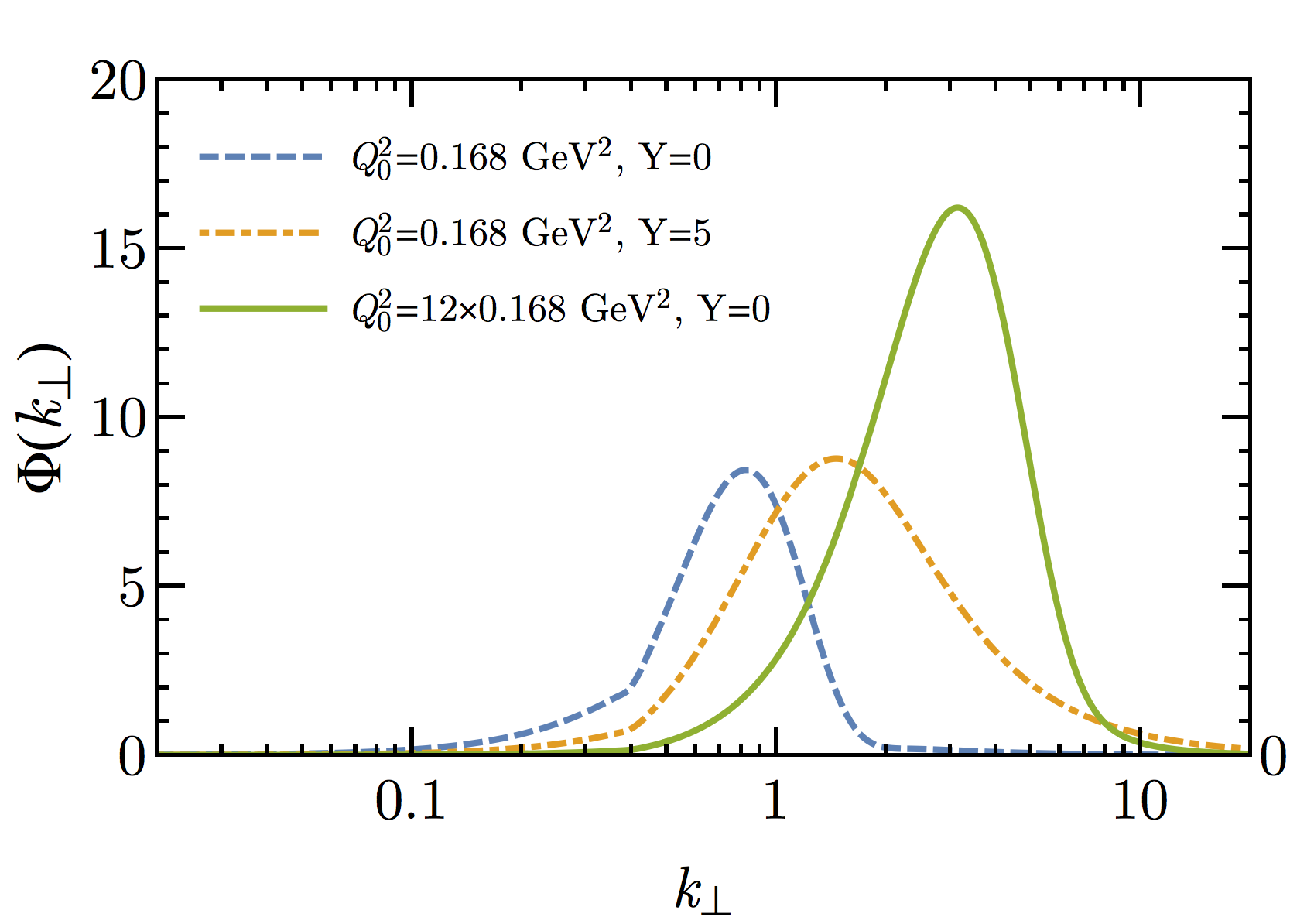
In order to obtain ridges, one needs to supply $C_{2}(\boldsymbol{p},\boldsymbol{q})$ with UGDs that are approximately bell-shaped curves which peak around the saturation scale $p_{\perp}\sim Q_{\mathrm{s}}$. So far, we have not yet mentioned which UGDs could be used for $C_{2}(\boldsymbol{p},\boldsymbol{q})$. The derivation of $C_{2}(\boldsymbol{p},\boldsymbol{q})$ is indeed independent of which UGD one wants to use as long as they have the aforementioned features. We will utilize the UGDs evolved by the rcBK equation; they include gluon saturation and are roughly bell-shaped curves with their peaks around $Q_{\mathrm{s}}$ (see Ref. [22]).

We find that $C_{2}(\boldsymbol{p},\boldsymbol{q})$ peaks at the azimuthal angle differences $\Delta\phi\sim 0$ and $\Delta\phi\sim\pi$

where $c$ is a constant. How $\cos(2\Delta\phi)$ structure (“double ridge”) arises from the glasma can be easily seen as follows. For this proof-of-concept calculation, instead of realistic rcBK UGDs, we shall use a mock Gaussian-shaped UGD

and we ignore the rapidity variable for the moment. We also rewrite the expressions in Eqs. (25), (26) and (27) in terms of azimuthal angles by using

where $p_{\perp}=|\boldsymbol{p}_{\perp}|$. The integration variable in Eq. (24) can be written as $d\phi_{k}dk_{\perp}k_{\perp}$. Since our mock UGD given in Eq. (29) peaks around $Q_{\mathrm{s}}$, we can make the substitution ${p_{\perp}\sim q_{\perp}\sim k_{\perp}\sim Q_{\mathrm{s}}}$ and get rid of the $dk_{\perp}$ integration. We ignore the rapidity coordinates $y_{p}$ and $y_{q}$ for the moment, and assume $A_{1}=A_{2}$. The azimuthal angles $\phi_{p}$ and $\phi_{q}$ are of the produced gluons whereas $\phi_{k}$ is to be integrated over. We define $\Delta\phi\equiv\phi_{q}-\phi_{p}$. We can rearrange our azimuthal coordinate system so that $\phi_{p}=0$, therefore the replacement $\phi_{q}=\Delta\phi$ can be made in Eq. (31). The only degree of freedom left is $\Delta\phi$. After carrying out the $\phi_{k}$ integration numerically for a list of values $\Delta\phi\in[0,2\pi]$, we verify the result given in Eq. (28) (see Fig. 3). This $\cos(2\Delta\phi)$ structure has been obtained numerically with rcBK UGDs in Refs. [21, 22, 23]. However, we note in passing that $\cos(2\Delta\phi)$ is not the only harmonic that exists in $C_{2}$. Although it is the dominant mode if the momenta of the tagged gluons are around $Q_{\mathrm{s}}$, different structures become visible as the transverse momenta and rapidities of the gluons are varied.

The away side ridge $(\Delta\phi\sim\pi)$ has contributions also from jet fragmentation and resonance decays. In Ref. [6], these contributions are removed and the double ridge structure became apparent in the data on p–Pb collisions $\sqrt{s}=5.02\;\mathrm{TeV}$. It has been observed that the near-side ridge ($\Delta\phi\sim 0$) was always accompanied with an identical ridge on the away side ($\Delta\phi\sim\pi$) (see Fig. 4), and this observation did not change with the systematics of event class and $p_{T}$ intervals of the measured hadrons. Also, based on the fact that the subtraction process is mostly independent of $p_{T}$, it has been concluded that the away-side ridge did not solely originate from the jet physics even though it included the jet and resonance decay contributions.

Although the glasma model is remarkably successful in explaining the ridges and reproducing their systematics in $N_{\rm track}$ and $p_{T}$ windows, there are other competing explanations which utilize the idea of final state collectivity (such as hydrodynamics) for p–p and p–Pb collisions, which has hitherto been thought to be impractical. At the moment, the di-hadron correlations are not enough to distinguish uniquely between the two scenarios leading to the ridges; final state collectivity or initial state effects by glasma. In order to settle this outstanding question, we suggest that one should look for possible ridges in triple-hadron, quadruple-hadron or even higher order hadron correlations. In the next section, we shall derive the triple-gluon $C_{3}(\boldsymbol{p},\boldsymbol{q},\boldsymbol{l})$ and quadruple-gluon $C_{4}(\boldsymbol{p},\boldsymbol{q},\boldsymbol{l},\boldsymbol{w})$ correlation functions for this purpose.

In this section, we calculate the triple-gluon correlation function at arbitrary rapidity and transverse momentum⁴⁴ 4 The triple-gluon correlation function that has been derived in Ref. [46] did not have rapidity and transverse momentum dependences since the charge densities $\mu^{2}_{A_{1,2}}$ therein have been taken to be constant. Hence, it is not suitable for calculating ridges in p–p and p–Pb collisions without resorting to collective flow in hydrodynamics sense.. Azimuthal collimations of ridges in tri-hadron and quadro-hadron correlations can be calculated from them.

The triple-gluon inclusive distribution can be written as

where

By using Eq. (4), we can write Eq. (32) in a compact way

where $\boldsymbol{r}_{i\perp}=(\boldsymbol{p}_{\perp},\boldsymbol{q}_{\perp},\boldsymbol{l}_{\perp})$ and

Here $\tilde{\rho}_{1}$’s and $\tilde{\rho}_{2}$’s can be contracted only among each other; i.e., there are no correlations between the charge densities of nucleus 1 (projectile) and nucleus 2 (target). For each of the projectile and target, there are $(2\times 3-1)!!=15$ contractions; hence, 225 diagrams in total. Examples of connected and disconnected diagrams are presented in Fig. 5. Here we shall only calculate the connected diagrams that are not power suppressed due to the contractions leading to extra delta functions, and at the same time non-vanishing in the limit of $\boldsymbol{p}_{\perp},\boldsymbol{q}_{\perp},\boldsymbol{l}_{\perp}\ll Q_{\mathrm{s}}$ (see Refs. [28, 46]). These are the rainbow diagrams where dimers of the same momentum are contracted among each other either on nucleus 1 or nucleus 2 [see Fig. 5(left)].

The disconnected diagrams are subtracted in the triple-gluon correlation function

Here $C_{3}(\boldsymbol{p},\boldsymbol{q},\boldsymbol{l})$ is the third cumulant, the first term on the right-hand side is the third moment, and the terms with the subscript “c” are the second cumulants, which are $C_{2}$’s. The cumulants include only the connected diagrams whereas the moments include both the connected and disconnected diagrams⁵⁵ 5 Alternatively, one can use the second moment rather than the second cumulant in the expansion of $C_{3}(\boldsymbol{p},\boldsymbol{q},\boldsymbol{l})$ as done in Ref. [46], and write ${C_{3}(\boldsymbol{p},\boldsymbol{q},\boldsymbol{l})=\left<d^{3}N_{3}\right>-3\left<d^{2}N_{2}\right>\left<dN_{1}\right>+2\left<dN_{1}\right>\left<dN_{1}\right>\left<dN_{1}\right>}$. The reason why we prefer the expansion in terms of cumulants rather than moments will be clear when we calculate the quadruple-gluon inclusive distribution. At that order, the naive cumulant expansion should be slightly modified so that the subtracted disconnected diagrams do not include the irrelevant diagrams which mix an upper and a lower disconnected two-gluon rainbow diagrams. These irrelevant diagrams are only partially in a rainbow form.. Let us first find out how many connected and disconnected rainbow diagrams the third moment has. There are $(2\times 3-1)!!=15$ contractions for each of the upper rainbow and lower rainbow. Both of these include the maximally disconnected diagram that is formed by three concentric circles. By avoiding double counting, we find there are 29 diagrams (connected and disconnected) in the third moment. We also know from the previous section that the second cumulant includes 4 diagrams. From Eq. (36), we can find the total number of diagrams included in $C_{3}(\boldsymbol{p},\boldsymbol{q},\boldsymbol{l})$

Since the experimentally relevant quantity is $C_{3}(\boldsymbol{p},\boldsymbol{q},\boldsymbol{l})$, we will only calculate these 16 diagrams that will lead us to $C_{3}(\boldsymbol{p},\boldsymbol{q},\boldsymbol{l})$.

In order to write ${\cal F}^{(3)}$ in terms of $\mu^{2}_{A_{1},A_{2}}$, we shall use the correlation functions given in Eqs. (19), (20) and (21) by keeping in mind that we now have one more rapidity variable $y_{l}$. The rapidity structure of these correlation functions are as follows. For correlations in $A_{1}$, $y_{p}$ will be chosen over $y_{q}$ and $y_{l}$, and $y_{q}$ will be chosen over $y_{l}$. For contractions in $A_{2}$, this ordering is reversed. Hence, for example

This pattern arises from our convention that the gluon with momentum $\boldsymbol{p}$ is close to the projectile, the one with momentum $\boldsymbol{l}$ is close to the target, and the one with momentum $\boldsymbol{q}$ is in between. Therefore, the rapidity ordering is $y_{p}>y_{q}>y_{l}$ (see also [28]).

After this point, the calculation proceeds similar to the cases of the single- and double-gluon calculations outlined before. The contractions between the color structure functions and the delta functions involving color factors give rise to a term $N^{3}_{c}(N^{2}_{c}-1)$. We skip the details of the tedious but straightforward calculations and show the final form of the triple-gluon correlation function⁶⁶ 6 Equation (12) in Ref. [27] does not reproduce correctly neither the prefactor of Eq. (41) here nor the momentum dependence of the UGDs in Eq. (44).

where

The prefactor in Eq. (41) follows a pattern in accordance with Eqs. (14) and (24). Note that we added the factor of two into the definitions in Eqs. (42) and (43). This factor of two arises from the diagrams which are mirror images of each other in the left-right direction. These pair of distinct diagrams, however, contribute precisely the same way.

In this section, we calculate the quadruple-gluon correlation function at arbitrary rapidity and transverse momentum. The procedure is identical to that of the triple-gluon calculation. At this order, there are $(2\times 4-1)!!\times(2\times 4-1)!!=11025$ diagrams in total. Some of the disconnected diagrams are shown in Fig. 6. We will only calculate the rainbow diagrams as mentioned in the previous section, and there are 96 of them at this order. This can be verified as follows. We first expand the fourth cumulant in terms of the third, second and first cumulants

where we used a compact notation; compare Eq. (45) with Eq. (36). The forth moment $\left<d^{4}N_{4}\right>$ contains

connected and disconnected diagrams, where the subtracted “1” is for the maximally disconnected diagram so that we do not double count it. We know from the previous sections that the cumulant $\left<d^{3}N_{3}\right>_{c}=C_{3}$ contains 16 diagrams, and the cumulant ${\left<d^{2}N_{2}\right>_{c}=C_{2}}$ contains 4 diagrams. From Eq. (45) we find the number of connected diagrams that $C_{4}$ contains

Although $\left<d^{2}N_{2}\right>_{c}$ contains 4 diagrams, note that the term $\left<d^{2}N_{2}\right>_{c}\left<d^{2}N_{2}\right>_{c}$ in Eq. (45) does not simply contribute $4\times 4=16$. This would be a mistake since we would have counted the disconnected diagrams which would include an upper rainbow from one of $\left<d^{2}N_{2}\right>_{c}$’s and a lower rainbow from the other one; these are not rainbow diagrams. This also tells us that the cumulant expansions of rainbow diagrams should be modified when necessary.

Since we already outlined the steps of the calculation of glasma diagrams in the previous sections, here we skip the details and only present the final result

where

References

- [1] Adrian Dumitru, Francois Gelis, Larry McLerran, and Raju Venugopalan. Glasma flux tubes and the near side ridge phenomenon at RHIC. Nucl.Phys., A810:91–108, 2008.
- [2] Vardan Khachatryan et al. Observation of Long-Range Near-Side Angular Correlations in Proton-Proton Collisions at the LHC. JHEP, 1009:091, 2010.
- [3] Drago Velicanu. Ridge correlation structure in high multiplicity pp collisions with CMS. J.Phys., G38:124051, 2011.
- [4] Wei Li. Observation of a ’Ridge’ correlation structure in high multiplicity proton-proton collisions: A brief review. Mod.Phys.Lett., A27:1230018, 2012.
- [5] Serguei Chatrchyan et al. Observation of long-range near-side angular correlations in proton-lead collisions at the LHC. Phys.Lett., B718:795–814, 2013.
- [6] Betty Abelev et al. Long-range angular correlations on the near and away side in -Pb collisions at TeV. Phys.Lett., B719:29–41, 2013.
- [7] Georges Aad et al. Observation of Associated Near-side and Away-side Long-range Correlations in TeV Proton-lead Collisions with the ATLAS Detector. Phys.Rev.Lett., 110:182302, 2013.
- [8] Leonardo Milano. Long-range angular correlations at the LHC with ALICE. 2014.
- [9] Betty Bezverkhny Abelev et al. Long-range angular correlations of pi, K and p in p–Pb collisions at TeV. Phys.Lett., B726:164–177, 2013.
- [10] Betty Bezverkhny Abelev et al. Multi-particle azimuthal correlations in p-Pb and Pb-Pb collisions at the LHC. 2014.
- [11] Betty Bezverkhny Abelev et al. Multiplicity dependence of jet-like two-particle correlations in p-Pb collisions at = 5.02 TeV. 2014.
- [12] Piotr Bozek. Collective flow in p-Pb and d-Pd collisions at TeV energies. Phys.Rev., C85:014911, 2012.
- [13] Piotr Bozek and Wojciech Broniowski. Correlations from hydrodynamic flow in p-Pb collisions. Phys.Lett., B718:1557–1561, 2013.
- [14] Piotr Bozek, Wojciech Broniowski, and Giorgio Torrieri. Mass hierarchy in identified particle distributions in proton-lead collisions. Phys.Rev.Lett., 111:172303, 2013.
- [15] K. Werner, M. Bleicher, B. Guiot, Iu. Karpenko, and T. Pierog. Evidence for flow in pPb collisions at 5 TeV from mass splitting. Phys.Rev.Lett., 112:232301, 2014.
- [16] Igor Kozlov, Matthew Luzum, Gabriel Denicol, Sangyong Jeon, and Charles Gale. Transverse momentum structure of pair correlations as a signature of collective behavior in small collision systems. 2014.
- [17] Adam Bzdak and Guo-Liang Ma. Elliptic and triangular flow in p+Pb and peripheral Pb+Pb collisions from parton scatterings. 2014.
- [18] Piotr Bozek. Elliptic flow in proton-proton collisions at TeV. Eur.Phys.J., C71:1530, 2011.
- [19] Adrian Dumitru, Kevin Dusling, Francois Gelis, Jamal Jalilian-Marian, Tuomas Lappi, et al. The Ridge in proton-proton collisions at the LHC. Phys.Lett., B697:21–25, 2011.
- [20] Kevin Dusling and Raju Venugopalan. Azimuthal collimation of long range rapidity correlations by strong color fields in high multiplicity hadron-hadron collisions. Phys.Rev.Lett., 108:262001, 2012.
- [21] Kevin Dusling and Raju Venugopalan. Evidence for BFKL and saturation dynamics from dihadron spectra at the LHC. Phys.Rev., D87(5):051502, 2013.
- [22] Kevin Dusling and Raju Venugopalan. Explanation of systematics of CMS p+Pb high multiplicity di-hadron data at TeV. Phys.Rev., D87(5):054014, 2013.
- [23] Kevin Dusling and Raju Venugopalan. Comparison of the color glass condensate to dihadron correlations in proton-proton and proton-nucleus collisions. Phys.Rev., D87(9):094034, 2013.
- [24] Raju Venugopalan. Long range correlations in high multiplicity hadron collisions:building bridges with ridges. 2013.
- [25] Raju Venugopalan. The ridge through colored glass. Nuclear Physics A, 2014. http://dx.doi.org/10.1016/j.nuclphysa.2014.08.071.
- [26] Jean Paul Blaizot, Francois Gelis, and Raju Venugopalan. High-energy pA collisions in the color glass condensate approach. 1. Gluon production and the Cronin effect. Nucl.Phys., A743:13–56, 2004.
- [27] F. Gelis, T. Lappi, and L. McLerran. Glittering Glasmas. Nucl.Phys., A828:149–160, 2009.
- [28] Kevin Dusling, Francois Gelis, Tuomas Lappi, and Raju Venugopalan. Long range two-particle rapidity correlations in A+A collisions from high energy QCD evolution. Nucl.Phys., A836:159–182, 2010.
- [29] Alex Kovner, Larry D. McLerran, and Heribert Weigert. Gluon production at high transverse momentum in the McLerran-Venugopalan model of nuclear structure functions. Phys.Rev., D52:3809–3814, 1995.
- [30] Yuri V. Kovchegov and Dirk H. Rischke. Classical gluon radiation in ultrarelativistic nucleus-nucleus collisions. Phys.Rev., C56:1084–1094, 1997.
- [31] Jamal Jalilian-Marian, Alex Kovner, Larry D. McLerran, and Heribert Weigert. The Intrinsic glue distribution at very small x. Phys.Rev., D55:5414–5428, 1997.
- [32] Jamal Jalilian-Marian, Alex Kovner, Andrei Leonidov, and Heribert Weigert. The BFKL equation from the Wilson renormalization group. Nucl.Phys., B504:415–431, 1997.
- [33] Jamal Jalilian-Marian, Alex Kovner, Andrei Leonidov, and Heribert Weigert. The Wilson renormalization group for low x physics: Towards the high density regime. Phys.Rev., D59:014014, 1998.
- [34] Jamal Jalilian-Marian, Alex Kovner, Andrei Leonidov, and Heribert Weigert. Unitarization of gluon distribution in the doubly logarithmic regime at high density. Phys.Rev., D59:034007, 1999.
- [35] Edmond Iancu, Andrei Leonidov, and Larry D. McLerran. Nonlinear gluon evolution in the color glass condensate. 1. Nucl.Phys., A692:583–645, 2001.
- [36] Edmond Iancu, Andrei Leonidov, and Larry D. McLerran. The Renormalization group equation for the color glass condensate. Phys.Lett., B510:133–144, 2001.
- [37] Elena Ferreiro, Edmond Iancu, Andrei Leonidov, and Larry McLerran. Nonlinear gluon evolution in the color glass condensate. 2. Nucl.Phys., A703:489–538, 2002.
- [38] Francois Gelis, Tuomas Lappi, and Raju Venugopalan. High energy factorization in nucleus-nucleus collisions. Phys.Rev., D78:054019, 2008.
- [39] Francois Gelis, Tuomas Lappi, and Raju Venugopalan. High energy factorization in nucleus-nucleus collisions. II. Multigluon correlations. Phys.Rev., D78:054020, 2008.
- [40] Francois Gelis, Tuomas Lappi, and Raju Venugopalan. High energy factorization in nucleus-nucleus collisions. 3. Long range rapidity correlations. Phys.Rev., D79:094017, 2009.
- [41] Larry D. McLerran and Raju Venugopalan. Computing quark and gluon distribution functions for very large nuclei. Phys.Rev., D49:2233–2241, 1994.
- [42] Larry D. McLerran and Raju Venugopalan. Gluon distribution functions for very large nuclei at small transverse momentum. Phys.Rev., D49:3352–3355, 1994.
- [43] Larry D. McLerran and Raju Venugopalan. Green’s functions in the color field of a large nucleus. Phys.Rev., D50:2225–2233, 1994.
- [44] Yuri V. Kovchegov. NonAbelian Weizsacker-Williams field and a two-dimensional effective color charge density for a very large nucleus. Phys.Rev., D54:5463–5469, 1996.
- [45] Sener Ozonder. Determination of the Parameters of a Color Neutral 3D Color Glass Condensate Model. Phys.Rev., D87(4):045013, 2013.
- [46] Kevin Dusling, Daniel Fernandez-Fraile, and Raju Venugopalan. Three-particle correlation from glasma flux tubes. Nucl.Phys., A828:161–177, 2009.
- [47] Francois Gelis, Anna M. Stasto, and Raju Venugopalan. Limiting fragmentation in hadron-hadron collisions at high energies. Eur.Phys.J., C48:489–500, 2006.
- [48] Hirotsugu Fujii, Francois Gelis, and Raju Venugopalan. Quark pair production in high energy pA collisions: General features. Nucl.Phys., A780:146–174, 2006.