Explicit Integration with GPU Acceleration for Large Kinetic Networks
Abstract
We demonstrate the first implementation of recently-developed fast explicit kinetic integration algorithms on modern graphics processing unit (GPU) accelerators. Taking as a generic test case a Type Ia supernova explosion with an extremely stiff thermonuclear network having 150 isotopic species and 1604 reactions coupled to hydrodynamics using operator splitting, we demonstrate the capability to solve of order 100 realistic kinetic networks in parallel in the same time that standard implicit methods can solve a single such network on a CPU. This orders-of-magnitude decrease in compute time for solving systems of realistic kinetic networks implies that important coupled, multiphysics problems in various scientific and technical fields that were intractable, or could be simulated only with highly schematic kinetic networks, are now computationally feasible.
Keywords:
ordinary differential equations , reaction networks , stiffness , reactive flows , nucleosynthesis , combustionPACS
02.60.Lj , 02.30.Jr , 82.33.Vx , 47.40 , 26.30.-k , 95.30.Lz , 47.70.-n , 82.20.-w , 47.70.Pq1 Introduction
Many important physical processes can be modeled by the coupled evolution of a reaction network (kinetic network) and fluid dynamics. A representative example is provided by astrophysical thermonuclear reaction networks, where a proper description of the overall problem typically requires multidimensional hydrodynamics coupled to the network across a spatial grid. Within each zone of the simulation the hydrodynamical (“hydro”) evolution controls the temperature and density, while the network influences the hydrodynamical evolution through energy release and composition changes. The solution of large kinetic networks by the usual implicit-integration approaches is slow and few calculations have attempted to couple the element and energy production strongly to the hydrodynamics with a network of realistic complexity. The most ambitious approaches use small schematic networks, perhaps tuned empirically to get critical quantities like energy production correct on average, coupled to the hydrodynamical simulation. Then a more physically realistic network is run in a separate “post-processing” step, where fixed hydrodynamical profiles computed in the hydrodynamical simulation with the schematic network are used to specify the variation of thermodynamic variables such as temperature and density with time.
Many other scientifically-interesting problems employ kinetic networks. Representative examples include the networks of chemical reactions required to model atmospheric chemistry, chemical evolution networks in contracting molecular clouds during star formation, plasma-surface interactions in magnetically confined fusion devices, fuel depletion in fission power reactors, and chemical burning networks in combustion chemistry. The corresponding reaction networks are large. Realistic atmospheric simulations, combustion of larger hydrocarbon molecules, studies of soot formation, core-collapse supernovae, and thermonuclear supernovae all can involve hundreds to thousands of reactive species undergoing thousands to tens of thousands of reaction couplings [1, 2]. Current techniques based on implicit numerical integration typically are not fast enough to allow coupling of realistic reaction networks to the full dynamics of such problems and even the most realistic simulations have employed highly schematic reaction networks.
As a representative example, the present situation in Type Ia supernova simulations is illustrated in Fig. 1.

A physically-realistic network is displayed in Fig. 1(a), a minimal physically-correct network for coupling to the hydrodynamical simulation is displayed in Fig. 1(b), and the current state of the art for Type Ia simulations employing multidimensional hydrodynamics is displayed in Fig. 1(c). The species omitted in reducing the 365-isotope network in Fig. 1(a) to the 150-isotope network in Fig. 1(b) are populated sufficiently weakly that they play little role in energy release and do not have significant influence on the coupling of the network to hydrodynamics. Thus, the 150-isotope network is a minimal network for coupling to the hydrodynamics; any network smaller than this will omit non-trivial parts of the realistic coupling between kinetics and fluid dynamics. The disparity between the minimal realistic network in Fig. 1(b) and the current state of the art in Fig. 1(c) is a consequence of insufficient computational power to couple a realistic kinetic network in real time to the fluid dynamics using current technology. This example from astrophysics is but one example of a number of problems from various fields of science and technology in which coupling realistic kinetics to fluid dynamics is hampered severely by insufficient computational speed for kinetic networks.
There are two general approaches that we might take to address the preceding issues. The first is to seek faster algorithms for solution of the typically large and stiff system of differential equations that describe the kinetic evolution. The second is to take advantage of advances in computational architectures to solve the chosen algorithm more rapidly. In previous work, [3, 4, 5, 6], we described a new algebraically-stabilized explicit approach to solving kinetics equations that extends earlier work by Mott [7] and is capable of taking stable integration timesteps comparable to those of standard implicit methods, even for extremely stiff systems of equations. Since the methods are explicit, they do not involve matrix inversions and thus scale linearly with network size. Because of this much more favorable scaling and competitive integration step size, we demonstrated that such algorithms are capable of performing numerical solution of extremely stiff kinetic networks containing several hundred species 5–10 times faster than the best implicit codes [3, 4, 5, 6].
One implication of new algorithms is that they may give new perspectives on optimization. Standard implicit methods spend most of their time on linear algebra operations for larger networks because they must be solved iteratively, which requires inversion of large matrices. Thus, the optimization strategy is clear for implicit algorithms: do the linear algebra faster. Conversely, the new explicit methods do not involve matrix inversions, so optimizing them involves different strategies. These may offer unique opportunities for implementation on newer architectures such as GPU or many-core accelerators coupled to standard CPUs [3]. In this paper we take a first step in addressing these issues by deploying the explicit integration methods described in our previous work [3, 4, 5, 6] on coupled CPU–GPU systems. We show that using GPUs to exploit the parallelism inherent in the explicit kinetic algorithm for networks of realistic size makes it possible find the solution for a single network on the GPU faster than on the CPU and the solutions for many networks simultaneously on the GPU versus serially on the CPU.
2 Implementation of Realistic Kinetic Networks
We shall assume that the coupling of reaction networks is done using operator splitting, where the hydrodynamical solver is evolved for a numerical timestep holding network parameters constant, and then the network is evolved over the time corresponding to the hydrodynamical timestep holding the new hydrodynamical variables constant (see §4 below). The general task for the kinetic network then is to solve efficiently coupled ordinary differential equations
| (1) | |||||
subject to initial conditions that have been determined in the current hydrodynamical timestep. In this expression, the describe the dependent variables (typically measures of abundance), is the independent variable (the time in our examples), the fluxes between species and are denoted by , and is the effective rate for all processes depleting the species . The sum for each variable is over all species coupled to by a non-zero flux , and for later convenience we have decomposed the flux into a component that increases the abundance of and a component that depletes it. For an -species network there will be such equations in the population variables , generally coupled to each other because of the dependence of the fluxes on the different . The variables are typically proportional to a number density for the species . For the specific astrophysical examples that follow we shall replace the generic population variables with the mass fraction , which satisfies
| (2) |
where is Avogadro’s number, is the total mass density, and is the atomic mass number for the species .
3 Algebraic Stabilization of Solutions Using Asymptotic Approximations
In the asymptotic limit we have for the species , leading to an approximate solution of Eq. (1) given by [4]
| (3) |
Since the asymptotic approximation specified above is expected to be valid if is large, we define a critical value of ( will be chosen here) and at each timestep cycle through all network populations and compute the product for each species and the proposed timestep . Then, for each population species
- 1.
If , the population is updated numerically by solving Eq. (1) using a standard explicit forward-Euler algorithm.
- 2.
Otherwise, for , the population is updated algebraically using the asymptotic approximation given in Eq. (3).
This algorithm is explicit, since all quantities required to update a timestep are available from the previous timestep. Thus, it avoids the iterative solution and associated matrix inversions required for implicit integration. As we have noted above, this algorithm alone implies as much as an order of magnitude increase in speed over standard implicit algorithms for solving realistic kinetic networks [3]. We shall demonstrate below that significant additional efficiencies are possible by using the GPU to exploit the parallelism inherent in the algebraically-stabilized explicit integration algorithm.
4 Operator-Split Integration Timesteps
In Fig. 2

the relationship of a hydrodynamical integration timestep (“hydro timestep”) to a kinetic network integration steps (“network timestep”) is illustrated for an operator-split simulation. The hydro integrator takes an adaptive timestep while the kinetic network is dormant. Then the updated hydrodynamical variables (temperature, density, …) are held constant while the kinetic network is integrated over the interval using adaptive network timesteps . The updated abundance variables and the energy released by the kinetic network are then passed from the kinetic network to the hydro integrator, which uses these and the equation of state to set the initial conditions for the next hydro integration timestep, and so on.
The hydro timestep and the network timestep are different timescales and should not be confused in the following discussion. The hydro timestep is set by characteristic times for response of the fluid while the network timestep is set by the inverse of the reaction rates in the kinetic network. For the examples discussed here, typically and the kinetic integrator might take 1–1000 network timesteps over the interval of one hydro timestep , depending on the ratio of characteristic kinetic reaction times to fluid response times in a given zone of the simulation. For our purposes, the hydro integration may be viewed as a black box to which the kinetic network is coupled by two-way transfer of information, and the only role of the current hydro timescale is to set the interval over which the kinetic network is to be integrated using adaptive timesteps .
5 GPU Acceleration
Modern supercomputers (as well as desktop and laptop systems) often have access to GPUs that can greatly accelerate the execution of algorithms formulated to take advantage of the parallelism exposed by the GPU. For example, Oak Ridge National Laboratory’s Titan supercomputer, which has been benchmarked at 17.59 petaflops and has a theoretical peak performance of 27.1 petaflops, employs 18,688 compute nodes, each consisting of 16 CPU cores and one NVIDIA Tesla K20X GPU, which uses the Kepler GPU microarchitecture [11]. The most powerful applications must integrate CPUs (each executing a few heavyweight threads) and GPUs (each executing many lightweight threads) seamlessly to reach speeds that are a significant fraction of the peak capability of the machine.
NVIDIA’s CUDA framework provides a parallel computing platform in which computational kernels written in CUDA C/C++ can be offloaded to the GPU from code running on the CPU. The CUDA programming model utilizes a heterogeneous memory paradigm in which a user first copies data from the CPU to the GPU using a special CUDA function, then launches a large number of threads, organized in blocks, which perform some computation. Thread blocks are distributed among streaming multiprocessors, which contain physical execution cores for integer and floating point operations along with registers, thread schedulers, and a cache, part of which can be accessed directly by the user as shared memory. Once kernel execution is complete, the user may copy data back to the CPU.
GPUs have various limitations that must be overcome to achieve large speedup from the massively-parallel, lightweight-thread implementation. Four issues are of particular importance:
- 1.
Data transfer between CPU and GPU is slow relative to compute speeds; thus scalable CPU–GPU computation must control the cost of communication between the CPU and GPU.
- 2.
Code running on GPUs must be highly parallel, since even small serial portions of a parallel code will greatly diminish performance (Amdahl’s Law).
- 3.
A modern general-purpose GPU typically has large amounts of relatively slow global memory and smaller amounts of much faster shared memory. For example, on a Tesla K20X GPU, each thread block has access to 6 GB of slow global memory and 48 KB of fast memory shared only within the block. Thus, optimal use of the GPU must enable a significant fraction of the calculation to use the fast, shared memory.
- 4.
The highest amount of performance is gained when as many as possible of the total number of threads on the GPU are used (“occupancy”).
Because of the simplicity and associated transparency of explicit integration algorithms and their intrinsically parallel nature for many of the required computing tasks, they are particularly attractive candidates for parallelization using GPUs. This task is greatly facilitated by the availability of computing platforms that allow high-level access to the GPU without the user having to deal with the details of thread management. In the applications discussed in this paper we have used NVIDIA CUDA C/C++ to implement algorithms that are launched under CPU control but that execute entirely on the GPU.
It is important to note that we do not present a detailed discussion on what the CPU can do with its free cycles. Ideally, the CPU would solve other coupled physics problems with these cycles in such a way that maximizes the amount of work done but minimizes the amount of time spent waiting for either piece of hardware to finish. However, it is also possible that the CPU could work on post-processing or uncertainty quantification. The easiest way to consume the cycles is to launch the GPU work asynchronously on a separate thread, possibly using OpenMP, and then do the CPU work.
6 Implementing the Explicit Asymptotic Algorithm on a CPU–GPU System
The prototype implementation that we shall describe here assumes an operator-split formulation of fluid dynamics coupled to a large kinetic network, with the computation of the fluid dynamics implemented on the CPUs and the computation of the kinetic networks implemented on the GPUs. This framework describes qualitatively a large number of potential scientific applications in a variety of fields, but to be definite we shall emphasize astrophysical thermonuclear networks coupled to hydrodynamical simulations in explosive burning scenarios. Our reference example will correspond to a 150-isotope network containing 1604 reactions (the minimal realistic network of Fig. 1(b)), integrated at a constant temperature of K and constant density of , but we shall display calculations with as many as 365 network species and 4300 reactions. In realistic simulations one often encounters approach to equilibrium and must use the asymptotic algorithm described above supplemented by a partial equilibrium approximation [3, 6]. Adding the partial equilibrium algorithm should not affect the parallelism of the problem substantially, so we shall simplify and illustrate using calculations not near equilibrium where the asymptotic approximation is sufficient.
In Fig. 3

we illustrate the basic structure of our example calculation. We shall refer to the code running on the CPU as the host and the code running on the GPU as the kernel in the following discussion. In a setup step that is executed once for each overall problem, library parameters required to calculate the temperature and density-dependent reaction rates are copied to the GPU and are resident on the GPU for the duration of the calculation. At the end of each hydrodynamical integration step a fully coupled CPU code would hold initial conditions for the kinetic network, which consists of the current temperature and density, and the current abundances for all species in the kinetic network. In a realistic simulation these values would be supplied to the CPU code by the hydrodynamical integration, but the source is irrelevant for our present tests and in our simulation we simply read in a trial set of initial conditions for a hydro timestep. One full kinetic network integration over a time interval corresponding to one hydrodynamical timestep then consists of the following steps.
- 1.
Copy from the CPU to the GPU (1) a vector of current network abundances, (2) the temperature, density, and duration of the current hydro timestep , and (3) a trial initial network timestep. For the representative 150-isotope network this corresponds to copying a total of 154 floating point numbers from the CPU to the GPU.
- 2.
Launch a GPU kernel to integrate the kinetic network over the time interval corresponding to the hydro timestep.
- 3.
When the integration on the GPU is complete, copy back to the CPU values of (1) the updated species abundances at the end of the kinetic network integration, (2) the integrated energy release over the kinetic network integration, and (3) a final kinetic network integration timestep for use in setting the initial trial timestep in the next network integration. For the representative 150-isotope network this corresponds to copying a total of 152 floating point numbers from the GPU to the CPU.
In this scheme, during the kinetic network integration corresponding to one hydrodynamical timestep (see Fig. 2) the network integration is done entirely on the GPU and the only communication between the CPU and GPU is at the beginning and end of the network integration. For the examples discussed here, the required data transfer between the CPU and GPU over each hydro integration step is thus 1 kB at the beginning and a similar amount at the end of each network integration. For typical installations the CPU–GPU data transfer rate is bytes per second, so each network integration over the interval of a hydro timestep requires a communication time that should be a negligible fraction of the total network integration time.
7 Performance for a Single Network
The accuracy of the GPU calculation relative to the reference CPU implementation of the algorithm used in Refs. [3, 4, 5, 6] has been tested for various networks containing from 14 to 365 isotopic species, in both single and double precision. This is illustrated in Fig. 4

for some arbitrarily selected species from the representative 150-isotope network integrated with double precision. It is clear that in double precision the GPU integration gives essentially the same results (typical differences between points and curves are less than one part in ) as the reference CPU implementation of the algorithm for mass fractions ranging over 20 orders of magnitude.
For GPU applications the limited amount of fast shared memory per block would make the use of single rather than double precision in the kinetic network highly advantageous, if it leads to stable and accurate results. We have tested single versus double precision implementations of the GPU algorithm. In general we find that for the conditions used in our tests (which are probably as extreme as for any kinetics simulation) the single-precision results are stable and more than accurate enough for coupling to fluid dynamics simulations. An example for the representative 150-isotope network is displayed in Fig. 5.

Thus we anticipate that considerable speed increase may be possible in a variety of applications by using single rather than double precision variables for the network, which allows more of the calculation to fit in the fast shared memory.
The execution time for the explicit asymptotic algorithm on several representative GPU installations for the case shown in Fig. 5 is displayed in Table 1.
| System | Microarchitecture | Time (s) | Steps | Time/Step (s) | Time/100 Steps (s) |
|---|---|---|---|---|---|
| Tesla M2090 | Fermi | 3.581 | 32,182 | ||
| Tesla K20X | Kepler | 5.910 | 32,182 | ||
| GT 640 | Kepler | 4.590 | 32,182 |
To put things on a common footing, we have divided the total integration time by the total number of integration steps and reported the average time to execute one network integration step in column 5. There is a range of almost two in speeds for different GPU microarchitectures, but we see that generally a GPU implementation is able to execute a kinetic integration step in - ms.
We may compare these results with representative explicit and implicit serial implementations of kinetic network integration on CPUs. For the example used in Table 1, the serial implementation of the explicit asymptotic algorithm [4] took seconds per kinetic integration step on a 3 GHz processor, which is not much longer than the GPU speeds displayed in Table 1. Although the GPU version is more parallel, the processors on the GPU are as much as 3–4 times slower than the CPU processor used, which partially offsets the parallelism advantage at the present level of optimization for the GPU code. We anticipate that with further optimization the explicit GPU code will become substantially faster than the corresponding CPU explicit code on present architectures.
For comparison with standard implicit methods we use as reference current implementations of the backward-Euler implicit code Xnet [8], which is a standard computational tool for solving thermonuclear networks in astrophysics and was the implicit-code reference used for comparisons in Refs. [3, 4, 5, 6]. We shall leave systematic comparisons aside until the explicit GPU code is more completely optimized, but some immediate quantitative comparisons are possible. We noted above that the current explicit serial CPU code is almost as fast as the GPU code at its current optimization. In Ref. [4] we used scaling arguments to predict that the serial (algebraically-stabilized) explicit algorithm should be able to integrate a 150-isotope network 5 or more times faster than an implicit algorithm on the same architecture because of faster computation of each timestep. Currently the implicit code using a sparse-matrix solver requires 0.5–1.0 ms per integration step on a CPU for integration of the representative 150-isotope network, depending on whether one or two Newton–Raphson iterations are required in an integration step (use of non-sparse methods for a 150-isotope network would be times slower) [9]. Thus, with the fastest GPUs in Table 1 the 150-isotope network appears to be executing 5–10 times faster on a GPU than current implicit codes running on a CPU.
The last column in Table 1 displays the time to execute 100 network integration steps using the explicit asymptotic GPU solver, which would be a representative number of kinetic network timesteps required in one hydro timestep for problems of the kind discussed here. Since the total time of this integration is ms, this suggests that a realistic kinetic network coupled to another physics solver could be executed in a time that will not slow the integration of the other physical system to a debilitating degree.
8 Scaling with Network Size for a Single Network
Fig. 6

shows the scaling of execution time for a single network integration step with network size. In Fig. 6(a) we compare the GPU version of the explicit asymptotic algorithm with a serial version of the same algorithm run on a standard 3 GHz CPU. We see that the speeds are comparable for small networks (with the serial code somewhat faster) but the parallel GPU version is approximately twice as fast as the serial version for 150 isotopes and almost three times as fast for 365 isotopes. Although the GPU version is aided by added parallelism, this is partially offset by the greater speed of the CPU processor versus GPU processors.
In Fig. 6(b) we make an approximate comparison of the parallel GPU explicit asymptotic algorithm with a standard backward Euler implicit integrator as a function of network size. We obtained the implicit curve by multiplying the serial explicit CPU curve in Fig. 6(a) by the scaling factors computed as a function of network size in Ref. [4], which give the ratio of the times to compute a single step for implicit and explicit methods, with because of the added matrix overhead of the implicit algorithm. The scaling of this curve could vary by factors of several because of variables such as the numerical solver used for the implicit method and the relative number of timesteps required in the implicit and explicit solves; however, with the present assumptions we see that for small networks the speeds are comparable but the explicit GPU calculation becomes considerably faster than the implicit calculation as network size increases. For 150 isotopes it is times faster, and for 365 isotopes the GPU code is times faster than the serial implicit calculation. We note that the explicit GPU scaling advantage of approximately 9 for a 150-isotope network inferred from Fig. 6(b) is consistent with the estimate made above based on current calculations with the implicit backward Euler code Xnet, giving some confidence in the validity of the comparison in Fig. 6(b).
Comparison of Fig. 6(a) and Fig. 6(b) indicates that the significant speed advantage of the GPU code for larger networks has two sources: (a) the explicit algorithm itself is faster per timestep for larger networks than implicit algorithms, as documented in Refs. [4, 5, 6, 3], and (b) the GPU implementation of the explicit algorithm is faster than the serial implementation of the same algorithm because of the enhanced parallelism of the GPU code, which is sufficient even at the present early stage of optimization to outweigh the slower speed of the GPU processors.
9 Multiple Parallel Networks and Thread Occupancy
The preceding examples indicate that a single realistic kinetic network can be integrated entirely on the GPU, with minimal communication overhead since CPU–GPU transfer of only a small amount of data at the beginning and end of the integration is required. This is already a substantial advance, since this implies that fast realistic fluid dynamics coupled to kinetic network simulations are now possible with the kinetic network running entirely on the GPU, freeing almost all CPU cycles for implementing the fluid dynamics. However, implementing a single network on the GPU is a woefully poor utilization of available threads since it basically engages only one of the available streaming multiprocessors. It is not easy to increase GPU thread occupancy in the solution of a single network because the network solution requires synchronization at several places (see Fig. 3). Without returning to the CPU, this can be enforced only within a single block containing a maximum of 1024 threads using present technology. However, it is desirable to run more than one network at a time on the GPU because in typical applications the CPUs of a compute node having a GPU will host multiple fluid dynamics zones and each zone has an independent network reflecting the conditions in that zone. Thus, we have tested running many networks in parallel on a single GPU, as illustrated schematically in Fig. 7.
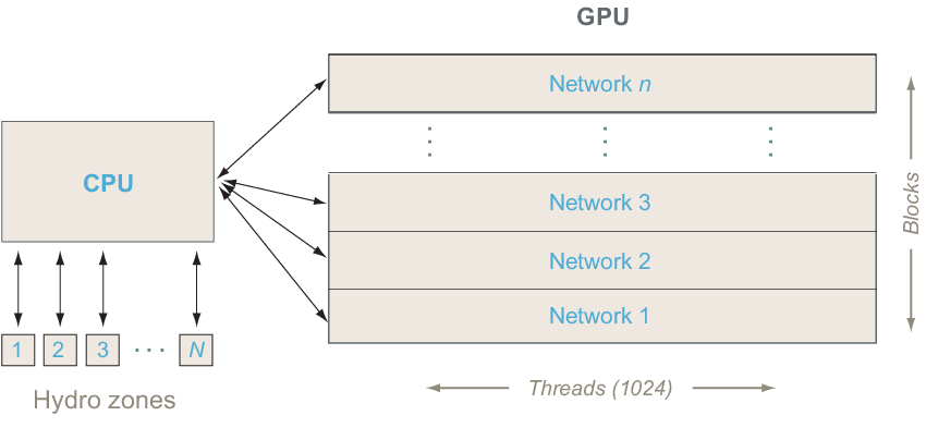
In our tests of concurrent execution of the reaction network kernel we deploy a number of OpenMP threads, with one asynchronous kernel launched by each thread after a small amount of processing on the CPU to prepare data for copying to the GPU. Timings are taken using the CUDA events timer and are started before thread creation and ended after all threads have joined. Thus the timing includes CPU processing and copying overhead as well as kernel execution time. Timing results for the launch of many representative 150-isotopes networks running in parallel are displayed in Fig. 8.

We see that the time to run networks scales almost perfectly (it is essentially the time to run a single network) up to . The time to run 15–28 networks is then about twice the time to run a single network, the time to run 29–42 networks is about three times the time to run a single network, and so on. The period of 14 concurrent networks in the steps reflects the availability of 14 streaming multiprocessors on the Kepler GPU microarchitecture. (The step period was found to be 15 when tested on a GPU using the Fermi GPU microarchitecture with 15 streaming multiprocessors available.) The slight rise in execution time on any given step presumably reflects a small increase in CPU overhead associated with launching increasing numbers of networks concurrently.
The results implied by Fig. 8 have large implications for simulations in a variety of scientific fields. They demonstrate that not only can a single realistic network be run fast enough now to couple to fluid dynamics, but in fact many such networks can execute in a short enough time to make the simulation feasible. The results presented in this paper are far from optimized (for example, we have only skimmed the surface of implementing efficient memory access), so we shall save detailed benchmarking for future papers. However, based on the results presented here (see Fig. 6 and Fig. 8 and the discussion associated with Table 1), and those of Refs. [3, 4, 5, 6], we may estimate that even without further optimization 14 realistic 150-isotope networks can now be run on a GPU in perhaps 10–20% of the time that a standard implicit code running on a CPU can integrate one such network, and that 100 realistic 150-isotope networks could be run in parallel entirely on a GPU in the same length of time that a standard implicit code could run one such network on a CPU.
Implicit algorithms are more complex than explicit algorithms because of the required iteration and matrix inversions. It remains to be seen whether they they can implement GPU versions having the same runtime qualities and low-memory footprint of this explicit method. In particular, problems with matrices of dimension a few hundred are memory bound because of a small number of computations relative to data required compared with problems with large matrices. To date, ports of the implicit code Xnet [8] to combined CPU–GPU architectures run only part of the calculation on the GPU, and do not give appreciable increase in performance over implementations on the CPU alone [9]. Recent tests of an accelerated batched LU factorization of matrices using the MAGMA library hybrid CPU–GPU algorithm have demonstrated speed increases as large as a factor of [10], but those methods remain to be fully implemented in Xnet [9].
The utility of these developments for realistic simulations is apparent. In an operator-split implementation of a zone-based fluid dynamics plus kinetics simulation, one could deploy the zones of the fluid dynamics on the CPUs of the compute nodes and the corresponding kinetic networks on the GPUs of the compute nodes (with one CPU per node allocating a small fraction of cycles to GPU management). Then the GPU can execute independent kinetic networks in parallel for many of the fluid dynamics zones at once in a short enough time to make the calculation with realistic networks in many zones feasible.11 1 The parallel network launches on a given GPU are asynchronous. To simplify this proof of principle the concurrent networks all were assigned the same temperature, density, and initial abundances, and so took the same number of integration steps. In a realistic application the concurrent networks in different zones typically would have the same reaction structure but perhaps different abundances and rates because of different conditions in each zone. Thus they may require varying numbers of integration steps and so might not return at the same time. The management of the network kernel launches can presumably be used to optimize workflow and load balancing in the coupled fluid dynamics and kinetic calculation. We have not explored these issues yet. This goes far beyond the current limitations of being able to execute only a highly-restricted number of unrealistically small kinetic networks coupled to the fluid dynamics, and plausibly enables a variety of simulations with realistic kinetics that previously were not accessible with available computing power.
10 GPU Virtues and the Explicit Approach
Let us revisit the four issues listed earlier in §5 that require particular attention for the efficient utilization of GPU acceleration. As we have shown, the simplicity of the explicit approach has permitted us to address these issues in a highly expeditious manner.
(1) Because the explicit method is compact, it is easy to fit entirely on the GPU so that no CPU–GPU communication is required except to launch the kernel and retrieve the results at the end of the calculation. Furthermore, the required data transfer at the beginning and end is minimal (of order a few kB for the representative examples shown here). Thus, there is little CPU–GPU communication penalty, even for the launch of multiple concurrent networks.
(2) The explicit algorithm is naturally highly parallel. The calculation of rates from the rate library expressions is a very parallel operation since the rates are all independent and need be calculated only once for each network integration.22 2 In the operator splitting approximation that we are employing the temperature and density are held constant during the network integration, so the rates also remain constant during the network integration steps corresponding to one hydro timestep and need be calculated only once per hydro timestep. The calculation of fluxes must be done at each network integration step (fluxes are products of rates and population variables; rates are constant but populations change with time in the integration), but that is also highly parallel since the fluxes are independent. The least parallel part of applying the algebraically-stabilized explicit asymptotic algorithm is that the sums of fluxes populating and depopulating a given isotope (the and of Eq. (1)) are required in order to compute the asymptotic update at each network timestep, and these summations are not intrinsically parallel. However, we have used tree methods to implement them, which can in principle attain execution times for the sum of fluxes. (We are far from that scaling now, presumably because our memory accesses are not yet optimized.)
(3) Even with double precision it is possible to fit most of the important variables into fast shared memory because of the compactness of the algorithm. We have also demonstrated that single-precision integration is stable and sufficiently accurate for many applications, which permits placing roughly twice as many variables in shared memory. For example, all relevant variables should fit in shared memory for the 150-isotope network in single precision.
(4) We have demonstrated that one can greatly increase thread occupancy by launching multiple networks concurrently. Thus the explicit method applied to multiple parallel networks scales to use all of the GPU streaming multiprocessors.
11 Future Work
It is our intention to develop the present technology into an open-source, general-purpose code for solving physically-realistic kinetic networks in a variety of disciplines. Although the present results are a substantial step in that direction, several important pieces remain to be implemented.
- 1.
The present implementation uses only the explicit asymptotic algorithm. This is adequate far from equilibrium but as systems approach equilibrium the asymptotic algorithm must be supplemented by a partial equilibrium algorithm to continue to scale [6]. Implementation of the asymptotic plus partial equilibrium algorithm requires only some flux modifications and some additional bookkeeping, neither of which should have much impact on parallelism, so we do not anticipate major issues with implementing it.
- 2.
The present algorithm is not well optimized with respect to memory access patterns. We anticipate that additional work on this issue will lead to a substantial increase in speed. The most significant source of concern in this area is coalescing memory accesses in order to prevent serialization caused by uncoalesced memory. It may be useful to utilize the GPU’s texture memory, which features a dedicated read-only cache optimized for spatial locality in a texture’s coordinate system rather than memory locality.
- 3.
We have shown that these calculations are stable and accurate with single-precision integration. This should allow less memory usage and faster calculations than double-precision integration, but this has not yet been fully explored.
- 4.
The least parallel part of the algorithm is the summation of fluxes changing the population of each isotope in each integration step. It is likely that this piece of the algorithm can be improved by restructuring, with a corresponding increase in speed.
- 5.
There are load-balancing issues associated with the flux summations that we have yet to address, occurring because the different isotopes in the network can require very different numbers of fluxes to be summed. For example, in the larger networks used here protons, neutrons, and 4He each have hundreds of fluxes that change their populations and must be summed, whereas almost all of the other isotopes in the network have fewer than ten. Presumably considerable optimization can be attained by a more load-balanced implementation of the flux summation algorithm.
- 6.
The explicit Quasi-Steady-State (QSS) algorithm is similar to the asymptotic algorithm and may in some cases give better CPU integration performance than the asymptotic algorithm [5]. It will be of interest to see if replacement of the asymptotic algorithm with the QSS algorithm in the present code leads to improved GPU performance.
- 7.
This paper has dealt with using GPU accelerators to implement the kinetics integration. We intend to port the current algorithm to systems with many-core accelerators, which we anticipate will also permit much more ambitious calculations than have been possible before.
- 8.
This work did not explore the benefits of overlapping computation and communication but it must be reviewed in the future.
Work is in progress on these improvements and we expect to report on them in future papers.
12 Summary and Conclusions
We have demonstrated that newly-developed explicit integration algorithms exhibiting many properties that are more desirable than those of implicit methods for large networks, coupled with multithreaded acceleration on GPUs, may permit orders of magnitude decreases in the runtimes to simulate large and realistic reaction kinetic networks that can be coupled to other physics solvers. Furthermore, we have demonstrated that for finding the solutions of many networks simultaneously the GPU far exceeds the performance of the CPU and its specific performance depends on the available number of streaming multiprocessors. These properties may make it possible to solve realistic coupled physics problems where the reaction network solve is the limiting factor. Finally, we described the future work that will be required to fully realize the performance benefits of using a GPU on these problems.
Readers interested in obtaining the source code should contact the corresponding author directly.
13 Acknowledgements
We thank Taro Yamaguchi-Phillips, Raph Hix, Bronson Messer, Austin Harris, Tom Papatheodore, and Reuben Budiardja for discussions; and David Bernholdt, Alexander J. McCaskey, and Phil Roth from Oak Ridge National Laboratory (ORNL) for thoroughly reviewing the manuscript and suggesting many helpful corrections.
This work has been supported by the US Department of Energy, Office of Nuclear Physics, and by the ORNL Undergraduate Research Participation Program, which is sponsored by ORNL and administered jointly by ORNL and the Oak Ridge Institute for Science and Education (ORISE). ORNL is managed by UT-Battelle, LLC, for the US Department of Energy under contract no. DE-AC05-00OR22725. ORISE is managed by Oak Ridge Associated Universities for the US Department of Energy under contract no. DE-AC05-00OR22750.
References
- [1] Oran E S and Boris J P 2005 Numerical Simulation of Reactive Flow (Cambridge: Cambridge University Press)
- [2] Hix W R and Meyer B S 2006 Thermonuclear kinetics in astrophysics Nuc. Phys. A 777, 188-207
- [3] Mike Guidry, J. Comp. Phys. 231, 5266-5288 (2012). [arXiv: 1112.4778].
- [4] M. W. Guidry, R. Budiardja, E. Feger, J. J. Billings, W. R. Hix, O. E. B. Messer, K. J. Roche, E. McMahon, and M. He, Comput. Sci. Disc. 6, 015001 (2013) [arXiv: 1112.4716].
- [5] M. W. Guidry and J. A. Harris, Comput. Sci. Disc. 6, 015002 (2013) [arXiv: 1112.4750]
- [6] M. W. Guidry, J. J. Billings, and W. R. Hix, Comput. Sci. Disc. 6, 015003 (2013) [arXiv: 1112.4738]
- [7] Mott D R 1999 New Quasi-Steady-State and Partial-Equilibrium Methods for Integrating Chemically Reacting Systems PhD thesis University of Michigan at Ann Arbor
- [8] Hix W R and Thielemann F-K 1999 Computational methods for nucleosynthesis and nuclear energy generation J. Comp. Appl. Mathematics 109 321-51
- [9] J. A. Harris; private communication
- [10] Dong, Tingxing, Haidar, Azzam, Luszczek, Piotr, Harris, J. Austin, Tomov, Stanimire, Dongarra, Jack. (2014). LU Factorization of Small Matrices: Accelerating Batched DGETRF on the GPU. Paper presented at the 16th IEEE International Conference on High Performance Computing and Communications (HPCC 2014), Paris, France, August 20-22, 2014.
- [11] June 2014 | TOP500 Supercomputer Sites. 10 Sept. 2014. Web. June 2014. http://www.top500.org/lists/2014/06