Correlations in the low-density Fermi gas:
Fermi-Liquid
state, Dimerization, and BCS Pairing
Abstract
We present ground state calculations for low-density Fermi gases described by two model interactions, an attractive square-well potential and a Lennard-Jones potential, of varying strength. We use the optimized Fermi-Hypernetted Chain integral equation method which has been proved to provide, in the density regimes of interest here, an accuracy better than one percent. We first examine the low-density expansion of the energy and compare with the exact answer by Huang and Yang (H. Huang and C. N. Yang, Phys. Rev. 105, 767 (1957)). It is shown that a locally correlated wave function of the Jastrow-Feenberg type does not recover the quadratic term in the expansion of the energy in powers of , where is the vacuum -wave scattering length and the Fermi wave number. The problem is cured by adding second-order perturbation corrections in a correlated basis. Going to higher densities and/or more strongly coupled systems, we encounter an instability of the normal state of the system which is characterized by a divergence of the in-medium scattering length. We interpret this divergence as a phonon-exchange driven dimerization of the system, similar to what one has at zero density when the vacuum scattering length diverges. We then study, in the stable regime, the superfluid gap and its dependence on the density and the interaction strength. We identify two different corrections to low-density expansions: One is medium corrections to the pairing interaction, and the other one finite-range corrections. We show that the most important finite-range corrections are a direct manifestation of the many-body nature of the system.
pacs
67.30.-n, 67.30.em, 71.10.Ca, 71.15.Qe, 71.45.GmI Introduction
The study of ultracold quantum gases is interlinked with controlling magnetic Fano-Feshbach resonances and thereby changing the effective interparticle interaction by many orders of magnitudes [1, 2, 3, 4, 5]. This makes ultracold Fermi gases a convenient tool to study the behavior of a degenerate fermionic many-body system [6] over a wide range of interaction strengths, in particular fermionic superfluidity [7, 8, 9, 10, 11]. Changing the magnetic field across a resonance makes it possible to continuously tune the gas from the Bardeen-Cooper-Schrieffer (BCS) state of Cooper pairs to a Bose-Einstein condensate (BEC) of weakly bound molecules. After the first observations of a molecular BEC of fermions [12, 13, 14], this so-called BCS-BEC cross-over has been widely studied experimentally [8, 15, 16, 9, 17, 18, 19] and theoretically [20, 21, 22], see also reviews Refs. 23, 24. The observation of quantized vortices on both sides of the BCS-BEC cross-over provided an unambiguous proof of superfluidity by fermionic pairing [25]. Recent work investigated the effect of partial polarization of a two-component Fermi gas on the Fermi liquid parameters [26], the nature of the transition from a BCS state to a state of a molecular BEC [27], and quantifying the superfluid fraction in a Fermi gas by means of second sound [28].
We study in this work the low-density properties of homogeneous Fermi gases at zero temperature. We use for our study a square-well and a Lennard-Jones interaction potential. Changing the interaction strength (coupling constant) of the respective potential changes the scattering length for two-body scattering , which we refer to as vacuum scattering length. The in-medium scattering length will be introduced later. When , i.e. the interaction is effectively attractive, one expects BCS type pairing of particles with opposite spin. As , a low energy resonance of the two-body problem generates bound dimers. is called the unitary limit, since the only relevant length scale is the inverse Fermi wave number . Increasing the attraction further, the Cooper pairs become bound molecules and the fermionic nature of their constituents becomes less visible.
We are in particular interested in structural quantities such as the energetics, distribution functions, the stability of the system against spinodal decomposition, dimerization, and BCS pairing. We utilize a quantitative method of microscopic many-body theory to determine correlation effects, i.e. effects beyond the weak coupling or mean-field approximations [29] that are routinely applied at low densities.
In the low density limit, many quantities like, for example, the ground state energy, depend only on the dimensionless parameter [30, 29]. We are interested here in the parameter range where this “universal” behavior ceases to persist due to correlation effects. An example for correlation effects is the pair distribution function, . In mean–field approaches, is equal to the distribution function of the non-interacting Fermi gas, . As we will see below, deviates, in particular for spin-antiparallel particles, substantially from when the absolute value of the scattering length becomes large compared to the characteristic length of the interaction potential.
In the limit of weak attractive interactions, the system can be described by a BCS type wave function. When the weak-coupling approximation does not apply (for example for Lennard-Jones type interactions), the pairing gap can be obtained by an extension of the Jastrow-Feenberg variational method. The correlated BCS (CBCS) method [31, 32] is reviewed in section III.1, see also Refs. 33, 34, 35 for a similar implementation of the same ideas. The CBCS theory takes into account short-ranged correlations analogously to the theory for normal systems, and supplements these by the typical BCS correlations. In its essence, CBCS provides a recipe for calculating an effective interaction that enters the standard BCS formalism. An alternative way to deal with the problem is a full Fermi Hypernetted Chain (FHNC) summation for large gap parameters has been suggested by Fantoni [36, 37], we will comment on this approach further below.
Our paper is organized as follows: In Sec. II we will review briefly the basics of the correlated basis functions (CBF) method. We call this approach “generic” many-body theory because the same equations can be derived from Green’s functions approaches [38], from Coupled Cluster theory [39] and from an extension of density functional theory which includes pair correlations. We evaluate in section II.2 the low-density limit and show that the exact formula [30] is not reproduced by the Jastrow-Feenberg and/or the “fixed node” approximation. To correct this problem, we apply in section II.3 perturbation theory in a correlated basis. We show that second-order CBF corrections must be added to obtain the correct low–density expansion.
In Sec. III.1 we will review the CBCS theory. We will show that the theory can be formulated in exactly the same way as ordinary BCS theory. CBCS simply provides a prescription for deriving weak, effective interactions from a strong, bare interaction. Upon closer inspection, the mapping of the bare interaction to an effective interaction is closely related to the transition from the bare interaction to the -matrix used in the low-density expansion of BCS theory [40, 41, 42].
In Sec. IV, we present our results for the energy, the pair distribution function, the in-medium scattering length, and the gap energy as a function of Fermi wave number and the vacuum scattering length . The dynamical correlations can be characterized by three regimes: For short distances, , these correlations are, of course, determined by the interaction. The intermediate regime is dominated by two-body scattering where correlations decay as . A third, asymptotic regime for larger than the average interparticle distance is dominated by many-body effects where the correlations decay as .
We find an instability of the FHNC-Euler-Lagrange (FHNC-EL) solutions accompanied by a divergence of the in-medium scattering length . This instability occurs well before the divergence of the vacuum scattering length ; it is caused by the induced interaction mediated by phonon exchange. Thus, strongly bound dimers can be formed at finite density even if the bare potential does not have a bound state. Note that this is a property of the normal system, wave functions of the type normally used only in the “BEC” regime [43, 44, 45] would here be more appropriate. We will return to this point further below.
In the regime we solve the CBCS gap equation and show that deviations from the simple BCS approximation can be separated into two contributions. One stems from the density dependence of the in-medium scattering length, the other one from the non-negligible momentum dependence of the pairing interaction in the CBCS gap equation.
II Generic Many-Body Theory
II.1 Variational wave functions
We start our discussion with the Jastrow-Feenberg theory for a strongly interacting, translationally invariant normal system. As usual, we assume a non-relativistic many-body Hamiltonian
| (1) |
where is a phenomenological, local interaction. The method starts with a variational ansatz for the wave function [46]
| (2) | ||||
| (3) | ||||
| (4) |
is a model state, normally a Slater-determinant for fermions and for bosons, and is the correlation operator written in the form (3). There are basically two ways to deal with this type of wave function. In quantum Monte Carlo studies, the wave function (2) is referred to as “fixed node approximation”. An optimal correlation function is obtained by stochastic means [43, 47, 44, 45, 48, 49, 50, 51, 52, 53, 54]. A decomposition into -body correlations is then, of course, not necessary. Alternatively, one can use diagrammatic methods, specifically the optimized Fermi-hypernetted chain method for the calculation of physically interesting quantities. These diagrammatic methods have been successfully applied to such highly correlated Fermi systems as 4He and 3He at [55]. They are naturally expected to work much better in the low density systems of interest here. In fact, we have shown in recent work [56] that even the simplest version of the FHNC-EL theory is accurate within better than one percent at densities less than 25 percent of the ground state density of liquid 3He.
Diffusion Monte Carlo calculations typically use a parametrized Jastrow-Feenberg (JF) ansatz for importance sampling, where the parameters are optimized by variational Monte Carlo calculations. JF theory makes explicit use of the form (3). It has been shown [38] that triplet correlations contribute to the ground state energy only in fourth order of the interactions. Even in strongly interacting quantum fluids like the helium liquids, triplet correlations contribute no more than five to ten percent to the ground state energy [57, 55] in both isotopes. They are completely negligible below approximately 25 percent of the respective equilibrium densities. We can identify, at the low densities we are concerned with here, the Jastrow-Feenberg approximation with the fixed-node approximation in quantum Monte Carlo calculations.
The correlations are obtained by minimizing the energy, i.e. by solving the Euler-Lagrange (EL) equations
| (5) | |||
| (6) |
The evaluation of the energy (5) for the variational wave function (3) and the analysis of the variational problem are carried out by cluster expansion and resummation methods. The procedure has been described at length in review articles [58, 55] and pedagogical material [32]. In any approximate evaluation of the energy expectation value, it is important to make sure that the resulting equations are consistent with the exact variational determination of the correlations. It has turned out that the (Fermi-)hypernetted chain hierarchy of approximations is the only systematic approximation scheme that preserves the properties of the exact variational problem [46].
Here, we spell out the simplest version of the equations that is consistent with the variational problem (“FHNC-EL//0”). These do not provide the quantitatively best implementation [55]. Instead, they provide the minimal version of the FHNC-EL theory. In particular, they contain the relevant physics, namely the correct description of both short- and long–ranged correlations. They also are the minimal implementation of the theory that gives the correct expansion of the ground state energy in powers of for the wave function Eq. (2).
In the FHNC-EL//0 approximation [59], which contains both the random phase approximation (RPA) and the Bethe-Goldstone equation in a “collective” approximation [32], the Euler equation (6) can be written in the form
| (7) |
where is the static structure factor of the interacting system, is the kinetic energy of a free particle, is the static structure of the non-interacting Fermi system, and
| (8) | |||||
is the so-called “particle-hole interaction”. We have also above defined the “Clark-Westhaus effective interaction” [58]. As usual, we define the Fourier transform with a density factor,
| (9) |
Auxiliary quantities are the “induced interaction”
| (10) |
and the “direct-direct correlation function”
| (11) |
Eqs. (7)–(11) form a closed set which can be solved by iteration. Note that the Jastrow correlation function (3) has been eliminated entirely.

The pair distribution function can generally be written as
| (12) |
Roughly speaking, describes dynamic, short-range correlations, is the pair distribution function of the non-interacting Fermi gas, and is the Slater exchange function. describes the combination of statistical and dynamic correlations. In leading order in the dynamic correlations we have
| (13) |
where is represented by the two exchange diagrams shown in Fig. 1.
In this approximation, the energy per particle is [55, 56],
| (14) | |||||
| (15) | |||||
| (16) |
where is the Fermi energy of non-interacting particles. is the degree of degeneracy of the single particle states; in our case we have generally . The term is the three-body term of the Jackson-Feenberg kinetic energy. The function is the sum of all three-point diagrams that have an exchange path connecting points and and no exchange lines attached to point which is dynamically connected in such a way that there exists a path between and each of the other two external points that does not go trough the third external point. The term is normally numerically very small; we must keep it here for the purpose of deriving the low-density expansion. To obtain the correct low-density limit, we retain all contributions to with two factors :
| (17) | |||||
The term cancels exactly the contribution to originating from the second diagram in ; the terms , and can then be combined to
| (18) |
The term is recognized as the three-body term of the “Clark-Westhaus” form of the kinetic energy. To summarize, the total energy has the form
| (19) |
For further reference, we also spell out the pair distribution functions in the spin-parallel and the spin-antiparallel channel:
| (20) | ||||
| (21) | ||||
| (22) |
where indicates the Fourier-transform (9). To leading order in the density, the term is the only term that reflects Fermi statistics, whereas the factor describes dynamical correlations. , , and are normalized such that they go to unity for large .
II.2 Low-density limit
In the limit of low densities, the equation of state and related quantities depend only on the vacuum -wave scattering length and the Fermi wave number . For example, the energy per particle has the expansion [30, 29]
| (23) |
Note that the expansion (23) is strictly valid only for . For attractive potentials the superfluid condensation energy must be added.
The locally correlated wave function (2) is not exact, and the question arises whether it recovers the expansion (23). It is plausible that this is not the case: The calculation of the third term in Eq. (23) makes explicit use of the form of the energy denominator in second order perturbation theory [29]. The local correlation operator corresponds to a “collective approximation” in which, among others, the particle-hole propagator is approximated by a collective mode.
Our task is to express the variational energy expression (19) to second order in the vacuum scattering length . One can deal with this task in two ways: One is to permit hard-core interactions, the other, somewhat simpler, approach is to assume a weak interaction that has a Fourier transform. In this case, one can parallel the derivation of Ref. 38 for fermions.
We will show the details of the calculation in Appendix A.1, here we discuss only the essential steps: The vacuum scattering length is determined from the zero-energy scattering equation
| (24) |
The scattering equation has the asymptotic solution
| (25) |
Multiplying Eq. (24) with and using the identity
| (26) |
gives a relationship that will be useful later:
| (27) |
The quantity is structurally identical to as introduced in Eq. (8), except that is calculated for the zero energy vacuum scattering solution . Integrating Eq. (27) leads to the relationship
| (28) | |||||
We notice that the induced interaction as defined in Eq. (10) is of second order in the interaction. To leading order in the density we can also expand Eq. (7)
and obtain from Eq. (11) the solution
| (29) |
In addition to calculating the energy contributions (19) for the correlation function (29), we must express in terms of the scattering length because is calculated with the optimal correlation function (11) of the many-body problem at finite density, and not with the solution of the zero-density scattering equation (24). In Appendix A.1 we will prove the relationship
| (30) | |||||
Collecting all results, one finds
| (31) |
see Appendix A.1 for details of the calculation. The result (31) is to be compared with the factor of Eq. (23). To get the exact result, one must go beyond local correlation operators; this is done by perturbation theory in a correlated basis generated by the correlation operator described in the next section II.3. The situation is analogous to the case of the high-density limit of the correlation energy of the electron gas. With local correlations one obtains for the logarithmic term 0.05690Ry [61] instead of the exact value 0.06218Ry [62, 63]. This deficiency is, for the electron gas, removed by second-order CBF theory [64]. One conclusion of our analysis is that the fixed node approximation in conjunction with Green’s functions [47] or Diffusion [44, 45] should reproduce the expansion (31) and not (23).
II.3 Elements of Correlated Basis Functions
We have seen above that a locally correlated wave function (2) does not produce the exact low-density limit (23) of the ground state energy. As mentioned above, the problem can be cured by applying second-order perturbation theory with correlated basis functions (CBF theory). We will also need the basic ingredients of CBF theory for examining the superfluid state. We review the method only very briefly, details may be found in pedagogical material [32] and review articles [58, 55]. The diagrammatic construction of the relevant ingredients has been derived in Ref. 65.
CBF theory uses the correlation operator to generate a complete set of correlated and normalized -particle basis states through
| (32) |
where the form a complete basis of model states, normally consisting of Slater determinants of single particle orbitals. Although the are not orthogonal, perturbation theory can be formulated in terms of these states [66, 46].
For economy of notation, we introduce a “second–quantized” formulation of the correlated states. The Jastrow–Feenberg correlation operator in (3) depends on the particle number, i.e. (whenever unambiguous, we omit the corresponding subscript). Starting from the conventional that create and annihilate single particle states, new creation and annihilation operators of correlated states are defined by their action on the correlated basis states:
| (33) | |||||
| (34) |
According to these definitions, and obey the same commutation rules as the creation and annihilation operators and of uncorrelated states, but they are not Hermitian conjugates. If is an –particle state, then the state in Eq. (33) must carry an -particle correlation operator , while that in Eq. (34) must be formed with an –particle correlation operator .
In general, we label “hole” states which are occupied in by , , , and unoccupied “particle” states by , , etc.. To display the particle-hole pairs explicitly, we will alternatively to the notation use . A basis state with particle-hole pairs is then
| (35) |
For the off–diagonal elements of an operator , we sort the quantum numbers and such that is mapped onto by
| (36) |
From this we recognize that, to leading order in , any depends only on the difference between the states and , and not on the states as a whole. Consequently, can be written as matrix element of a -body operator
| (37) |
(The index indicates antisymmetrization.)
The key quantities for the execution of the theory are diagonal and off-diagonal matrix elements of unity and ,
| (38) | |||||
| (39) |
Eq. (39) defines a natural decomposition [65, 32] of the matrix elements of into the off-diagonal quantities and and diagonal quantities .
To leading order in the particle number, the diagonal matrix elements of become additive, so that for the above -pair state we can define the CBF single particle energies
| (40) |
with where
| (41) |
and is an average field that can be expressed in terms of the compound diagrammatic quantities of FHNC theory. According to (37), and define particle operators and , e.g.
| (42) | |||||
Diagrammatic representations of and have the same topology [65]. In homogeneous systems, the continuous parts of the are wave numbers ; we abbreviate their difference as .
In principle, the and are non-local -body operators. In the next section, we will show that we need, for examining pairing phenomena, only the two-body operators. Moreover, the low density of the systems we are examining permits the same simplifications of the FHNC theory that we have spelled out in Sec. II.1. In the same approximation, the operators and are local, and we have [55]
| (43) |
The most straightforward application of CBF theory is to calculate corrections to the ground state energy. In second order we have, for example,
| (44) |
The magnitude of the CBF correction is normally comparable to the correction from three-body correlations [55]. It is also important to note that there are significant cancellations between the two terms in the numerator. We will show in appendix A.1 that the CBF correction (44) corrects the coefficient of the third term in the expansion (31) and leads to the exact low-density limit (23).
III BCS Theory with correlated wave functions
III.1 General derivation
We show in this section how the variational theory is generalized to a superfluid or superconducting state. We restrict ourselves here to the simplest case of –wave pairing and show how the effective interactions, which enter phenomenological theories as parameters, may be calculated from first principles. This section reviews the derivations of Refs. 31, 32.
The BCS theory of fermion superfluidity generalizes the Hartree–Fock model by introducing a superposition of independent particle wave functions corresponding to different particle numbers [67]
| (45) |
The coefficient functions and are known as Bogoliubov amplitudes. They describe the distortion of the Fermi surface due to the pairing phenomenon.
To deal with strongly interacting systems, adequate provision must be made for the singular or near–singular nature of the two–body interaction for small interparticle distances . To build the required geometrical correlations into the microscopic description of the system, we can define a correlated BCS state, incorporating both short-ranged and BCS correlations. We are faced with a formal mismatch, which prevents us from simply applying the correlation factor to . The former is defined in the –particle Hilbert space and the latter is a vector in Fock space with indefinite particle number. The most natural way to deal with this is first projecting the bare BCS state on an arbitrary member of a complete set of independent–particle states with fixed particle numbers, applying the correlation operator to that state, normalizing the result, and finally summing over all particle numbers. We must therefore distinguish between correlation operators and normalization integrals corresponding to different particle numbers . Thus, the correlated BCS (CBCS) state is
| (46) | |||||
The trial state (46) superposes the correlated basis states with the same amplitudes with which the model states enter the corresponding expansion of the original BCS vector.
To derive the relevant equations we consider the expectation value of an arbitrary operator with respect to the superfluid state:
| (47) |
One may pursue cluster–expansion and resummation methods of expectation values (47) for the superfluid trial state (46). This has been done successfully for the one– and two–body density matrices corresponding to a slightly different choice of the correlated BCS state [36] which exhibits, unfortunately, divergences for optimized correlation functions. We do not follow this route, but instead consider the interaction of only one Cooper pair at a time. The error introduced by this is of order , where is the superfluid gap energy. We will demonstrate below that this quantity is indeed small in the regime where the wave function (46) is appropriate.
In leading order, it is sufficient to retain the terms of first order in the deviation and those of second order in . We refer to this as the “decoupling approximation”. The calculation of for correlated states [31] is somewhat tedious, we only give the essential steps and the final result. It is convenient to introduce the creators and annihilators of correlated Cooper pairs,
| (48) |
In terms of these quantities, the expectation value of an operator is, to leading order in the amplitudes and
| (49) | |||||
In Eqs. (49), the operators , , and are the , , and –particle realizations of the operator , and the expectation value of the operator in the –particle correlated ground state. Inserting for into the expansion (49), where is a Lagrange multiplier (the chemical potential) introduced to adjust the average particle number , we recover the effective interactions, overlap integrals (42), and single–particle energies (41) of section II.3, e.g.
| (50) | |||||
| (51) | |||||
| (52) | |||||
Accordingly, we may write the energy of the superfluid state in the form
| (53) |
with the “pairing interaction”
| (54) | |||||
With the results (53) and (54), we have arrived at a formulation of the theory which is formally identical to the BCS theory for weakly interacting systems. Upon closer inspection (see the next section) we will see that our formulation corresponds to a BCS theory formulated in terms of the scattering matrix [41]. The correlation operator serves here to tame the short–range dynamical correlations. The effective interaction is just an energy independent approximation of the -matrix.
We may proceed now in the conventional way to determine the Bogoliubov–amplitudes , , by variation of the condensation energy (53) to compute the superfluid condensation energy or to investigate the local stability of the normal ground state by second variation. Minimization of the energy expectation value determines the BCS amplitudes , . The CBCS gap equation becomes
| (55) |
The conventional, i.e. uncorrelated, BCS gap equation [68] is retrieved by replacing the effective interaction by the matrix elements of the bare interaction. Note that our “decoupling approximation” simply means that we assume that the pairing interaction does not depend on the Bogoliubov amplitudes.
To conclude this section, we point to a subtle issue concerning the normalization of the correlated BCS state (46). Above, we have written the wave function as a specific linear combination of normalized states . In our formulation of a correlated pairing theory [34] as well as in related work [36, 37] the correlated BCS state
| (56) |
where
| (57) |
is the BCS state (45) projected into the -particle Hilbert space. This approach leads to a slightly different gap-equation where the gap function under the square root in Eq. (55) is scaled by a factor , see Eq. (3.16) od Ref. 34. This factor diverges for optimized or otherwise long-ranged correlations. To avoid this divergence we have used here the method developed in Ref. 31.
III.2 Analysis of the gap equation
In the local approximations appropriate for low densities, the effective interaction is given by Eqs. (43). The pairing matrix element is expressed in terms of the Fourier-transforms and :
| (58) |
The remaining arguments are standard, cf. Ref. 68, 41: If the gap at the Fermi surface is small, we can replace the pairing interaction by its -wave matrix element at the Fermi surface,
| (59) |
Then we can write the gap equation as
| (60) | ||||
which is almost identical to Eq. (16.91) in Ref. 41. In particular, the second term has the only function to regularize the integral for large . We can, therefore, immediately conclude that the zero temperature gap is, in this approximation, given by
| (61) |
with
| (62) |
The low-density limit is then obtained by identifying with the vacuum scattering length :
| (63) |
Of course, our equations (54), (55) are much more general: At low densities, the subtraction term – i.e. the second term in the square bracket of Eqs. (58) and (60) is important to regularize the integral for large momentum transfers. At higher densities, the finite range of the interaction provides that momentum cutoff and the subtraction term becomes negligible since the energy numerator term is zero at the Fermi momentum.
By comparison with the low-density limit and Eq. (28) we interpret the constant
| (64) |
as an “in-medium” scattering length. Hence, at finite densities, one expects two types of corrections:
- (i)
Medium corrections: The effective pairing interaction is related to through Eqs. (7)- (11) which leads to
(65) Because of Eq. (30) and the fact that the induced interaction is of second order in the interaction, we conclude that that
(66) In the same order, non-local contributions to the pairing interaction (43) [65] contribute. These can be identified with particle-hole ladder diagrams and vertex corrections. Topologically, one of these diagrams corresponds to the polarization correction identified by Gorkov et al. [40]. Moreover, similar to our analysis of the low-density limit, local correlation functions will not get the right coefficient of the term proportional to , hence CBF corrections to the pairing interaction [31] will also lead to modifications of order .
- (ii)
The solution of the -wave gap equation is dominated by the matrix element (59) of at the Fermi surface which leads to the solution (61). Only if is practically constant for , we can identify with the in-medium scattering length . The dominant finite-range correction to the pairing interaction comes from the kinetic energy term . For interparticle distances much larger than the interaction range , but smaller than the average particle distance, this term is dominated by the vacuum solution of the Euler equation, . For interparticle distances larger than , we obtain from Eqs. (7) and (11) that falls off like
(67) Consequently, the effective interaction is quadratic in for and has a linear dependence
(68) for . The variation of the pairing interaction between and is interaction-dependent and causes, as we shall see in Sec. IV.3 a correction that is larger than the ones due to the effects mentioned above.
All of the corrections discussed above except the one due to the quadratic momentum dependence of for are order and higher i.e. thy lead to a density dependence of the in-medium scattering length of the form
| (69) |
where is a numerical constant. Among others, the polarization correction discussed by Gorkov [40] has this structure. Inserting the above expansion in (61) changes the pre-factor to
| (70) |
In other words, to the extent that an expansion in powers of is legitimate, all of these corrections just lead to a modified, but universal, pre-factor in Eq. (63). This does not apply to the finite-range correction of the pairing interaction in the relevant regime . One would, of course, expect that this finite-range correction is of the same order of magnitude. We shall see in Sec. IV.3 that its value depends, on details of the interaction. Hence, we conclude that the exponential behavior of Eq. (63) is universal whereas the pre-factor is not.
IV Results
IV.1 Energetics
We have examined in this paper two model potentials, namely a Lennard-Jones (LJ) potential
| (71) |
and an attractive square well (SW) potential
| (72) |
Both potentials are parametrized by a characteristic length and the depth of the attractive well . In both cases, we measure energies in units of , and length in units of . Thus, the interaction strength and the density are the only free parameters.
Our choice of interactions provides effective potentials designed to avoid the instability against clustering that exists for realistic alkali interactions, but otherwise be close to a realistic situation. The simplest connection to real interactions is provided by the vacuum -wave scattering length . The procedure is legitimate in the low-density limit, many observable properties of these gases, such as the energy (23), depend indeed only on the -wave scattering length [30, 29]. For higher densities this “universal” behavior ceases. It is the purpose of our calculation to explore that area, and also study the model dependence, by comparing results for the LJ and SW model. To make contact with low-density expansions, as well as to determine the range of “universal behavior”, we shall use the -wave scattering length instead of the well-depth to characterize the potential.
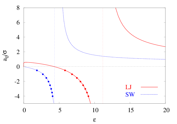
For the SW potential, is given by where . For the LJ potential, must be obtained numerically. We show in Fig. 2 as a function of the potential well depth . The attractive SW potential has negative scattering length for an interaction strength below the first resonance. The LJ potential has a positive below , indicating an effectively repulsive interaction. Thus, when the interaction strength of the LJ potential is raised, starting from , we find three regimes. (i) For we have and there is no bound state; the many-body ground state is a normal Fermi gas. (ii) For we have . There is still no two-body bound state. Due to the effectively attractive potential, the many-body ground state is, at low densities, a BCS state. (iii) At the LJ potential has a resonance at zero scattering energy. For , becomes positive again, and the potential supports at least one two-body bound state. All these states of Fermi gases have been studied extensively in experiments with ultracold alkali gases as discussed in the introduction. In a previous paper, [56] we have already studied both, and for fermions, and for bosons. In that work we have also examined more sophisticated versions of the FHNC-EL method and have concluded that these are necessary only at densities comparable to that of liquid helium. The reader is referred to that work to assess the range of densities for which the very simple version of the theory spelled out in Sec. II.1 is reliable. In short, the accuracy of our energy calculations is expected to be better than 1 percent below a density of , whereas the error of the simple FHNC-EL version is about 10 percent as the density increased to which is close to the freezing density of 3He.
We focus in the present work on the effect of attractive interactions (). We have solved Eqs. (7)-(11) on a mesh of points, with a resolution of 30 points between and , amounting to a box size of 8732. Such a huge box size is necessary to obtain a reasonable momentum space resolution at the very low densities we are considering here: Note that a Fermi wave number of corresponds to a wavelength of , hence this box size is the bare minimum of what one should take to resolve features of the order of the Fermi wave number. All our calculations are done for the range of interaction strength where there is no two-body bound state, i.e. before the first resonance of appears (indicated by vertical lines in Fig. 2).
Our equation of state for the two potential models is shown in Figs. 3 and 4. To recover the exact low-density limit (23), we have added the second-order CBF correction (44). To emphasize the interaction terms, we have subtracted the kinetic energy . We have normalized the equation of state to the expansion (23). Thus, Figs. 3 and 4 show only the model-dependent correction to the equation of state. Omitting the CBF correction (44) and comparing to the low-density expansion (31) gives practically the same results, they are therefore not shown.
Figs. 3 and 4 show already a visible dependence of the equation of state on the potential model at approximately where the third term in the expansion (23) is of the order of . In other words, for both interactions the model-dependent corrections are of the same order of magnitude as the third term in the expansion (23). For both interactions we observe that, dependent on the interaction strength, the equation of state begins to deviate strongly from a simple, smooth power law for .


The most interesting feature we observe is that the FHNC–EL equations cease to have solutions at sufficiently large values of the density or of . Such a limit is expected for sufficiently attractive interactions: The Fermi gas is, in the low density limit, stabilized by the Pauli pressure. As the density increases, the energy per particle becomes negative and the static incompressibility
| (73) |
where is the hydrodynamic speed of sound, goes to zero. Such an effect has already been reported by Owen [69]. indicates a spinodal instability, where the system separates into a low and a high density phase. On the other hand, it is widely accepted that a low density two-component Fermi gas is subject to dimerization close to the unitary limit, . In the following we will argue that dimerization indeed occurs, but well before the limit . Instead, dimerization is accompanied by the divergence of the in-medium scattering length.
Let us examine the question of stability from the point of view of the existence of solutions of the FHNC-EL equations: In general, the FHNC-EL equations cease to have solutions if the assumed wave function is unstable against small perturbations. This is most clearly seen for the case of density fluctuations: The term under the square root of Eq. (7) must be positive. In the limit this leads to the condition
| (74) |
The right-most expression is the low density limit, , where is small and the in-medium scattering length is well approximated by the vacuum scattering length , see Eq. (76). The limit can be regarded as the low density limit of the particle-hole interaction,
| (75) | |||||
We have used above the fact that the induced interaction is of second order in the bare interaction. Hence, the system can be driven into an instability by holding the potential fixed and simply increasing the density factor in Eq. (75). Note that the above stability limit (74) is valid for the local correlation operator (2). In an improved calculation that does not rely on a local correlation operators but rather includes CBF corrections to all orders [55] the stability condition would read
| (76) |
The condition is immediately recognized as the stability condition of Landau’s Fermi Liquid theory, . Note that the ground state theory formulated in Eqs. (7)-(11) does not contain self-energy insertions (called “cyclic-chain” diagrams in the FHNC theory), which means that the effective mass is equal to 1. According to our findings in Ref. 56, this is an acceptable approximation at the low densities under consideration here. Since the interaction contribution to is, at low densities, proportional to , an instability against density fluctuations could occur for sufficiently attractive interactions. This has the consequence that the FHNC-EL equations cease to have a solution.
We found indeed an instability of the solutions of the FHNC-EL equations. However, this instability does not appear to be caused by . In fact, in our calculations we were not able to come close to the point of spinodal instability. We show in Figs. 5 and 6 the value of as a function of density for a family of potential strengths. For the SW potential, we have, depending on the coupling strength , been able to solve the FHNC-EL equations in the regime between up to a critical density that depends on the coupling strength. At that density, begins to drop very rapidly but it does not appear to approach the critical value of for a spinodal instability, see Fig. 5. We also note that an instability signified means a transition to a state with non-uniform density which is not what has been observed experimentally.

Whereas a system of fermions interacting with an attractive SW potential exhibits an instability as the density is increased, the LJ model interaction leads, due to its repulsive core, to a richer phase diagram that also features a high-density condensed phase – the liquid phase of 3He. At low densities, we see the same picture as for the SW potential: The liquid is stabilized by the Pauli pressure, but the FHNC-EL equations cease to have solutions above a certain density where the Landau-parameter is still far from its critical value . The situation is different in the high-density regime: For sufficiently strong interactions, the system also can develop a high-density condensed phase. The noteworthy feature is that one can get much closer to the spinodal instability limit from higher densities than from lower densities.

To examine the nature of the instability, we show in Fig. 7 the in-medium scattering length , see Eq. (64). The ratio is shown as function of for increasing values of : for the SW model and for the LJ model. We do not show and for the LJ model, because the system is stable for all densities as discussed above. Similar to the vacuum scattering length, the in-medium scattering length exhibits a singularity. The location of the singularity depends obviously on both the density and the interaction model. Evidently, medium corrections to the effective interactions have the effect that the in-medium scattering length exhibits a singularity as is increasing. The larger , the smaller the critical value where the the divergence happens, see also Fig. 8. is universal only for very low densities, where all curves merge into a single curve converging towards unity in the zero density limit. For finite density, , and thus , depends on , , and the interaction model, and not just on the dimensionless parameter .
The appearance of such an effect is not surprising because the leading correction to the bare interaction is the attractive phonon-exchange. This leads, as the density is increased, to a divergence of the in-medium scattering length . Thus, we conclude that the instability found in our calculations is an indication of phonon-induced dimerization. Further evidence for the appearance of a phonon-exchange induced dimerized phase will be provided in the next section where we discuss distribution functions.

Figs. 7 show essentially the same scenario for the SW and the LJ model. At a given density, the critical scattering length where dimerization occurs is model-dependent. But the difference becomes smaller as the density is reduced. In order to determine the critical scattering length, we have extrapolated the in-medium scattering length to the point where it diverges. The result for both interactions are shown in Fig. 8. There we show the inverse of the critical scattering length where the normal state becomes unstable as function of . The curves for the LJ and the SW potential approach each other when is well below 0.1. This shows that the critical value of becomes universal in the low density limit. As a consequence of many-body effects, this critical value of is not zero.

The physical message that emerges here is actually quite simple: Normally the transition from a “BCS” state to a “BEC” state is discussed in terms of the vacuum scattering length ; it is clear that, as diverges, the expressions (63) or (70) for the gap become meaningless. To be rigorous, one should however use in these equations the in-medium scattering length and not the vacuum scattering length . We have justified this (see Eq. (65)), we have calculated the in-medium scattering length, and found a divergence of before the vacuum scattering length diverges. This is expected because many-body effects change the interaction, and the first correction term is attractive.
Similar dimerization effects have been observed in two-dimensional 3He-4He mixtures, in double-layers of bosonic dipoles [70], and also in the process of -clustering of nuclear matter [71, 72]. We hope that our result that there are clear many-body effects to be identified in the BCS regime will encourage experimental investigations in this regime.
IV.2 Distribution Functions
The pair distribution functions for parallel and anti-parallel spins, (20) and (21), contain information about correlations due to Fermi-statistics and, more interestingly, due to interactions. The latter are captured by the direct-direct correlation function , which we show in Figs. 9 for the LJ and SW model, respectively. The respective potential strengths were chosen such that the scattering length was . is shown for three Fermi wave numbers and . One can discern two regimes: the asymptotic regime where falls off as for due to many-body effects, see Eq. (67); and an intermediate regime where is smaller than the average particle distance and falls off like as expected from two-body scattering in vacuum. The behavior in the asymptotic regime can be obtained from the limit of Eqs. (7) and (11) which leads to Eq. (67). In the low-density limit, the speed of sound is obtained from the equation of state (23). Since only the speed of sound enters, the asymptotic form of is independent of the interaction model. In Figs. 9 this asymptotic behavior is illustrated by straight lines.

For low densities, the spin-parallel pair distribution function is dominated by Fermi statistics. The Pauli exclusion principle ensures that , regardless of interactions. This is guaranteed by the statistical factor in Eq. (20) which suppresses for , thus screening the interaction. Note also that . Therefore, the interaction effectively plays no role in a dilute gas of spin-polarized fermions, which has also been established in many experiments. For example for , the curves for obtained for the two interactions are almost indistinguishable from each other and from the distribution function of non-interacting fermions for a wide range of values of the vacuum scattering length between and . is essentially identical to the spin-parallel pair distribution of free fermions , which has also been verified by QMC results [44, 52]. Thus, little or no non-trivial information can be obtained from , and we therefore refrain from further discussing or showing this quantity.

The anti-parallel pair distribution function is not suppressed by statistical correlations. Instead, is dominated by correlation effects, which are described by the direct–direct correlation function , Eq. (11). The effectively attractive interaction, , leads to an enhancement of as is reduced. We show in Fig. 10 for and , for both the SW and the LJ potential. For small distances , is dominated by the interaction potential, leading to a large value at for the SW potential: The maximum value of is attained at . For the largest considered here, we have obtained solutions of the FHNC-EL equations where is more than 150 times larger than . The short range repulsion of the LJ interaction suppresses the pair distribution for , and therefore as . The maximum value of , which is attained at finite , is therefore much lower than in the SW case.
One might argue that both models are unrealistic at short , the shape of for is of only theoretical interest. However, we will show in Section IV.3 that finite-range effects have a quite visible effect on the superfluid energy gap and, hence, on the condensation energy. We also observe that for , becomes universal in the sense that it is independent of the choice of interaction. This is not a feature special to cold gases: The asymptotic behavior of is determined by the speed of sound [46], see also Eq. (67). is still strongly enhanced compared to the asymptotic limit . Furthermore we find that is very similar to the zero-energy scattering solution of the two-body Schrödinger equation, this is simply due to the fact that is dominated by the dynamic correlation function , cf. Eq. (21). The situation changes again as we approach the dimerization instability: The maximum value of starts to rise rapidly indicating an approaching singularity. The effect becomes stronger and appears at lower density as the coupling strength of the underlying bare interaction is increased.

IV.3 BCS pairing
We now return to the question of the density– and momentum dependence of the pairing interaction . We have discussed already above that the in-medium scattering length can become singular due to phonon-exchange correction, the considerations of this section apply therefore only to the case of weak pairing, in other words to a physical situation where the wave function (2) is a good approximation.
Before we describe our calculations, we go back to the momentum dependence of the pairing interaction. We show in Figs. 12 for two values of , (top panel) and (bottom panel). For small such as and less, the regime where behaves as is rather large. Therefore, the linear regime in is well defined and agrees well with the prediction (68). For , the regime where the behavior of the correlations is visible is much smaller, hence the linear regime is less well defined and also becomes model dependent. The important point to be made here is, however, that in neither case, and especially as gets larger, is the simple estimate from low-density expansions valid for a significant portion of the integration regime which is needed for the calculation of the -wave pairing matrix elements, see Eq. (59).

We have calculated the gap in the excitation spectrum at the Fermi surface, (see Eq. (55)), for the LJ and the SW interaction model, for a wide range of densities, characterized by the Fermi wave number , and -wave scattering lengths . A first overview is shown in Fig. 13, where the higher values of correspond to larger values of .

Figs. 13 provide two pieces of information: One is an assessment of the accuracy of the approximate solution (61). This is obviously quite good throughout the whole regime of interaction strengths and densities. The major difference comes, at high densities, from the deviation of the vacuum scattering length from defined in Eq. (62). The general dependence of the gap on both the interaction strength and the density is quite similar, in particular the exponential dependence on the scattering length holds over many orders of magnitude. This is consistent with the general feature spelled out in Sec. III.2 that medium– and finite–range corrections are manifested in the pre-factor in Eq. (70). This pre-factor is universal as long as the in-medium scattering length is of the form (69) which is the case, among others, if the momentum dependence of is linear. Deviations from this universal behavior can only be expected from the quadratic behavior of for which is a direct manifestation of many-body effects. Indeed, this correlation effect is significant: We show in Fig. 14 the ratio , see Eq. (62), in the density/interaction strength regimes where the gap is larger than . Evidently, the behavior is, in that regime, neither linear, nor a universal function of . Only at very small values of where the gap is of the order of , a linear behavior might be interpreted, but the slope of such a linear behavior depends on the interaction model. Calculations at even lower density where a linear regime might be found require a much bigger mesh than the one used here to reliably resolve the region .


In order to disentangle medium and finite-range corrections, we show in the right and left panels of Figs. 15 (LJ model) and 16 (SW model) the ratios and as defined in Eqs. (61) and (63), respectively, plotted as function of . The color of the symbols encodes the value of the corresponding data point, between red for and black for – the low density regime which usually is assumed to be universal in the sense that all quantities depend on only. Data for are not shown in these figures. The two ratios and give information on two different effects: The ratio is an assessment of the accuracy of the approximations leading to Eqs. (61) and reflects the importance of the momentum dependence of the pairing interaction. Evidently, this effect is visible and depends little on the density, the ratio does not seem to go to unity with decreasing density. This is simply a consequence of our findings of Figs. 12: No matter how small the Fermi momentum is, the momentum dependence of the pairing interaction is never given by the naive application (68) of low-density arguments but rather reflects genuine many-body physics. For the range of densities and coupling strengths, is between and , but there is a rapid drop of for , as the system becomes unstable against dimerization. In other words, neglecting the momentum-dependence of the pairing interaction, and thus the finite range of the interaction, leads to an overestimation of that becomes more severe as one approaches the dimerization instability. We also note that, apart for some values for large , collapses on a single curve, i.e. it is characterized by a universal dependence on . The curves are identical for the LJ and the SW model.
The difference between our microscopic calculation and the low-density expression (63) is much more visible, see the left panels of Figs. 15 and 16. This effect has, of course, to do with the divergence of the in-medium scattering length as discussed above. However, even far from the singularity, we see very little evidence of an approach to a “universal” behavior. Evidently one must go to much lower densities. We have been able to carry out our ground state calculations down to densities of . At such low densities, the gap itself becomes many orders of magnitude smaller than the Fermi energy, cf. Figs. 13. Calculations at even lower densities are therefore only of methodological interest.
V Summary
We have in this paper reported ground state calculations for low-density Fermi gases described by two model interactions, an attractive square-well potential and a Lennard-Jones potential. We have used the optimized Fermi-Hypernetted Chain integral equation method which has been proved to provide, in the density regimes of interest here, an accuracy better than one percent [56]. We have examined the low-density expansion of the energy for a local correlation operator, written in the conventional Jastrow-Feenberg form (2). Our formal results also apply for fixed-node Monte Carlo calculations for wave functions written in that form. Of course, such a result can only be obtained with optimized correlation functions. Using a parametrized Jastrow function instead leads to an unpredictable answer of which one can only say that it should lie above the expansion (31). We have demonstrated that a locally correlated wave function does not reproduce the exact low-density limit and have cured the problem by adding the second-order CBF corrections. We have also demonstrated that already at values of the third term in the expansion (23) is overshadowed by model-dependent corrections.
The most interesting result of our work is the appearance of a divergence of solutions of the FHNC-EL equations well before the divergence of the vacuum scattering length of the interaction potential. This makes a statement on both the physics we are describing and on many-body methodology.
The physics has been described at the end of section IV.1. In the simplest terms it says that the scattering length appearing in Eq. (61) should be replaced by the in-medium scattering length and that the relationship between and is non-universal and depends on many-body effects. Within the medium, the bare interaction is supplemented by the induced interaction , cf. Eq. (10) or (65), which describes phonon exchange. This density-dependent correction to the bare interaction changes the interaction strength at which a bound state appears. Thus, the appearance of a divergence of as a function of is expected: As a function of coupling strength, the vacuum scattering length has a singularity somewhat above the strength where we find the singularity. The closer the bare interaction is to the appearance of the bound state, the smaller the correction needs to be. Since the induced interaction depends on the density, the singularity appears at lower density for stronger interactions.
We have studied, in the stable regime, the superfluid gap and its dependence on the density and the interaction strength. Two corrections apply to low density expansions: medium corrections and finite-range corrections. We have shown that the most important finite-range corrections are a direct manifestation of the many-body nature of the system. For low densities, the gap can be reasonably well approximated by neglecting finite-range corrections but accounting for medium corrections, but the deviations from the full numerical solution increase on approaching the dimerization instability.
The second statement is about many-body methodology. The divergence of solutions of the FHNC-EL equations is in analogy to the spinodal instability discussed in Sec. 4A, and in many places in the earlier literature, that the (F)HNC-EL equations for the homogeneous system have no solutions if , i.e. if the system is unstable in the particle-hole channel. ( The fact that this does not come out exactly (see Eq. (4.4)) is a consequence of the “fixed node approximation” (2.2).) Here, we prove that the (F)HNC-EL equations have no solutions if the ground state is unstable against dimerization, i.e. if the system is unstable in the particle-particle channel. This is a unique feature of theories like FHNC-EL that have the topological completeness of parquet diagrams.
A more appropriate variational wave function for situations with strong pairing is perhaps an antisymmetrized product of pair functions as proposed, among others, in Refs. [33, 44, 73, 74]. It is well known that the projection of the BCS state onto a fixed particle number, i.e. the states can, in coordinate space, be written in such a form [75]. Unfortunately, such a -particle state does not lead, in the limit of weak coupling, to a BCS-type theory and a BCS equation (55). This is easily seen by considering the stability of the normal state. To make our point, it is sufficient to consider a weakly interacting system. To guarantee normalization, we express the Bogoliubov amplitudes in terms of the real phase angle : and . Now consider the stability of the normal ground state against pairing. For the original BCS state one obtains the familiar expression [67]
where is the normal Fermi distribution.
If we use, instead, the number-projected state we get
| (77) |
for and or vice versa, and zero otherwise. See Ref. 34, Eqs. (2.7), (2.8). Thus, the number-projected BCS state, while useful for strongly coupled pairs, i.e. typically beyond the first singularity of the (in-medium) scattering length, does not reproduce the correct stability condition in the weakly-coupled limit. Full optimization of such a wave function containing both Jastrow correlations and an antisymmetrized product of pair wave functions requires first to derive the diagrammatic expansion, which goes beyond the scope of this paper.
Appendix A Low-density expansions for fermions
A.1 Low density limit for local correlations
In the limit of low densities, the exact energy per particle is given by the expansion (23) [30, 29]. The wave function containing a local correlation operator (2) is not exact, it is of interest to determine the consequences of this approximation for the low-density expansion.
There are two ways to derive the low–density expansion for the wave function (2): One is to assume that the interaction is weak and has a Fourier transform. Then one can proceed in the same way as in Ref. 38, i.e.

- •
Derive the cluster-expansion of the energy keeping all terms that are (a) of second order in the correlation function , or (b) of first order in the potential and first order in the correlation function
- •
Derive the Euler equation and express the correlation function to first order in the potential
- •
Re-insert the optimal correlation function in the energy
- •
Collect all terms that can be written as powers .
If we also permit hard-core interactions, we must formulate the expansion in terms of the dynamical correlation function and take into account that the solution of the Euler equation is density dependent. The analytic expression for the relevant energy contributions is given in Eqs. (14), (15) and (18). The only additional simplification is that we can set, to leading order in , the factor in . The resulting diagrammatic representation of the energy expansion is shown in Fig. 17.
In the low-density limit, is much shorter ranged than both the exchange function and the dynamic correlation function . can therefore be replaced by its long–wavelength limit which is, in turn, related to the scattering length, see Eq. (30). Then, diagrams (b), (d), and (f) are times diagrams (a), (c), and (e), respectively. For the correlation function (29), all diagrams shown in Fig. 17 can be calculated exactly in terms of the long-wavelength limit . The calculation is somewhat tedious but straightforward and leads to the aforementioned result (31). However, this is not the exact solution because the exchange diagram (f) has not been treated exactly.
To derive the exact low-density limit, we start from the diagrammatic expansion up to second order is shown in Fig. 17. Carrying out the variation with respect to we get
| (78) |
where is represented by the two diagrams shown in Fig. 1, with the dashed line replaced by . In leading order in , we can replace and expand
| (79) | |||||
and similarly
| (80) |
Finally, we combine the last two terms in Eq. (78) to .
Multiplying the equation with , using
and keeping only first order terms in reduces Eq. (78) to
| (81) |
The approximation leading to Eq. (29) is to replace the third term by
This is legitimate if the range of is small compared to that of which is not necessarily true. To assess the importance of this term, we write
| (82) |
with as and as . In the long wavelength limit , the function becomes universal. We have solved the Euler equation (81) in that limit, the resulting function is shown in Fig. 18. The deviation from is small but visible. Calculating the energy correction to second order in leads to a coefficient instead of . The smallness of the effect is plausible because diagram (g) contributes only a few percent to the total energy correction.

A.2 Density Dependence of the Correlation Functions
We have in Eq. (82) derived the connection between the dynamical correlation function and the effective interaction . To complete the calculation of the low-density limit of the energy for local correlation operators, we must establish the connection between and the scattering length because is calculated with the optimal correlation function (82) of the many-body problem at finite density, and not with the solution of the vacuum scattering equation (24). To calculate the correction, let
Then
| (83) | |||||
The last line follows because is of order , and the mixed term is zero due to the scattering equation (24). Since we have eliminated the potentially singular bare potential, we can expand the kinetic energy term to get
| (84) |
Collecting all results, one finds
| (85) |
The numerical factor is to be compared with the factor of Eq. (23). We emphasize again that the result (31) also applies for the “fixed-node” approximation because the terms, where that approximation deviates from our expansion, are of at least fourth order in the potential strength.
A.3 Correlated Basis Functions Corrections
Once we have determined that a local correlation operator of the form (2) does not lead to the correct low-density limit (23) of the correlation energy, the question arises what corrections to that wave function are necessary. We show here that second-order CBF perturbation theory (44) is sufficient to retrieve the exact low-density expansion. In the low-density (local) approximation and are given by Eqs. (43).
There are normally significant numerical cancellations between the two terms in the numerator of Eq. (44). However, for the purpose of discussing formal properties, we may expand the numerator. The term containing two matrix-elements is just the ordinary expression of second-order perturbation theory [29]. None of the other terms contains an energy denominator, they can therefore be written in terms of the diagrams of the JF method.
We carry out the calculation for just the direct term (notice that the double-exchange is equal to the direct term):
| (86) | |||||
where , , and
| (87) |
Expanding the second term as
| (88) | ||||
we identify in the first term the negative diagram (e) and in the second term the negative diagram (c) of Fig. 17. Likewise, expanding the last term of Eq. (86) as
| (89) |
we identify in the first term the negative diagram (g) of Fig. 17. Thus, these terms cancel exactly all direct, two-line diagrams shown in Fig. 17.
The last terms in Eqs. (88) and (89) cannot be represented by legitimate diagrams of JF-theory, they are combined to
| (90) |
The first term is seen to cancel the correction (84). The second term is combined with the first term in Eq. (86) to give the textbook result [29]
The treatment of the exchange terms is done along the same lines and will not be repeated here.
Appendix B Numerical solution of the gap equation
B.1 General strategy
We present in this appendix details of our solution method for the gap equation which is numerically delicate.
The gap equation
| (91) |
is highly non-linear and a simple iteration procedure does not converge. For values , the integrand is narrowly peaked at the Fermi momentum and an adaptive mesh is necessary to reach a reliable numerical accuracy. Above, we have introduced the angular average
| (92) |
A very rapidly converging algorithm is as follows: Consider the generalized eigenvalue problem
| (93) | ||||
To shorten the equations, let
| (94) |
The problem can be mapped to a regular symmetric eigenvalue problem by defining
| (95) |
Then, the eigenvalue problem is
The algorithm is
- (i)
Start with a reasonable estimate , e.g. a constant
- (ii)
Solve the above eigenvalue problem as a function of the scaling parameter and find the value for which the lowest eigenvalue is 1. Along with a trial solution, we can calculate the derivative with respect to , see below.
- (iii)
Scale the corresponding eigenfunction such that .
- (iv)
Go to step (ii) and repeat until convergence which is obtained for .
B.2 Adaptive mesh
To deal with the strongly peaked denominator , we introduce a transformation that generates a dense set of points around the Fermi momentum. Then
| (96) |
Now find a function such that
| (97) |
is almost constant. The function of choice is
| (98) | |||||
| (99) |
where and . This choice has the property
| (100) |
i.e.
is almost constant.
We can also obtain a closed-form expression for :
| (101) |
Acknowledgements.
This work was supported, in part, by the College of Arts and Sciences, University at Buffalo SUNY, and the Austrian Science Fund Projects P21264 and I602 (to EK) and P23535 (to REZ). Additional support was provided by the Spanish Ministry of Science and Education (MEC) through project FIS2011-28617-C02-01 and from the Qatar National Research Fund # NPRP 5 - 674 - 1 - 114. Discussions with J. Boronat are also acknowledged.References
- [1] S. Inouye, M. R. Andrews, J. Stenger, H.-J. Miesner, D. M. Stamper-Kurn, and W. Ketterle, Nature 392, 151 (1998).
- [2] P. Courteille, R. S. Freeland, D. J. Heinzen, F. A. van Abeelen, and B. J. Verhaar, Phys. Rev. Lett. 81, 69 (1998).
- [3] E. Timmermans, P. Tommasini, M. Hussein, and A. Kerman, Phys. Rep. 315, 199 (1999).
- [4] S. Giorgini, L. P. Pitaevskii, and S. Stringari, Rev. Mod. Phys. 80, 1215 (2008).
- [5] C. Chin, R. Grimm, P. Julienne, and E. Tiesinga, Rev. Mod. Phys. 82, 1225 (2010).
- [6] K. M. O’Hara, S. L. Hemmer, M. E. Gehm, S. R. Granade, and J. E. Thomas, Science 298, 2179 (2002).
- [7] C. Chin, M. Bartenstein, A. Altmeyer, S. Riedl, S. Jochim, J. H. Denschlag, and R. Grimm, Science 305, 1128 (2004).
- [8] M. Bartenstein, A. Altmeyer, S. Riedl, S. Jochim, C. Chin, J. H. Denschlag, and R. Grimm, Phys. Rev. Lett. 92, 120401 (2004).
- [9] J. Kinast, S. L. Hemmer, M. E. Gehm, A. Turlapov, and J. E. Thomas, Phys. Rev. Lett. 92, 150402 (2004).
- [10] M. W. Zwierlein, C. H. Schunck, A. Schirotzek, and W. Ketterle, Nature , 54 (2006).
- [11] Q. Chen, C. A. Regal, M. G. D. S. Jin, and K. Levin, Phys. Rev. A 73, 041601/1 (2006).
- [12] S. Jochim, M. Bartenstein, A. Altmeyer, G. Hendl, S. Riedl, C. Chin, J. H. Denschlag, and R. Grimm, Science 302, 2101 (2003).
- [13] M. Greiner, C. A. Regal, and D. S. Jin, Nature 426, 537 (2003).
- [14] M. W. Zwierlein, C. A. Stan, C. H. Schunck, S. M. F. Raupach, S. Gupta, Z. Hadzibabic, and W. Ketterle, Phys. Rev. Lett. 91, 250401 (2003).
- [15] C. A. Regal, M. Greiner, and D. S. Jin, Phys. Rev. Lett. 92, 040403 (2004).
- [16] C. A. Regal, M. Greiner, S. Giorgini, M. Holland, and D. S. Jin, Phys. Rev. Lett. 95, 250404 (2005).
- [17] T. Bourdel, L. Khaykovich, J. Cubizolles, J. Zhang, F. Chevy, M. Teichmann, L. Tarruell, S. J. J. M. F. Kokkelmans, and C. Salomon, Phys. Rev. Lett. 93, 050401 (2004).
- [18] M. Greiner, C. A. Regal, and D. S. Jin, Phys. Rev. Lett. 94, 070403 (2005).
- [19] G. B. Partridge, K. E. Strecker, R. I. Kamar, M. W. Jack, and R. G. Hulet, Phys. Rev. Lett. 95, 020404 (2005).
- [20] M. Holland, S. J. J. M. F. Kokkelmans, M. L. Chiofalo, and R. Walser, Phys. Rev. Lett. 87, 120406 (2001).
- [21] E. Timmermans, K. Furuyab, P. W. Milonnia, and A. K. Kerman, Phys. Lett. A 285, 228 (2001).
- [22] M. G. Lingham, K. Fenech, S. Hoinka, and C. J. Vale, Phys. Rev. Lett. 112, 100404 (2014).
- [23] R. Duine and H. T. C. Stoof, Phys. Rep. 396, 115 (2004).
- [24] Q. Chen, J. Stajic, S. Tan, and K. Levin, Phys. Rep. 412, 1 (2005).
- [25] M. W. Zwierlein, J. R. Abo-Shaeer, A. Schirotzek, C. H. Schunck, and W. Ketterle, Nature 435, 1047 (2005).
- [26] N. Navon, S. Nascimbene, F. Chevy, and C. Salomon, Science 328, 729 (2010).
- [27] M. J. H. Ku, A. T. Sommer, L. W. Cheuk, and M. W. Zwierlein, Science 335, 563 (2012).
- [28] L. A. Sidorenkov, M. K. Tey, R. Grimm, Y.-H. Hou, L. Pitaevskii, and S. Stringari, Nature 498, 78 (2013).
- [29] L. D. Landau and E. M. Lifshitz, Statistical Physics, Course of Theoretical Physics, Vol. V (Pergamon Press Ltd., London - Paris, 1958).
- [30] K. Huang and C. N. Yang, Phys. Rev. 105, 767 (1957).
- [31] E. Krotscheck, R. A. Smith, and A. D. Jackson, Phys. Rev. B 24, 6404 (1981).
- [32] E. Krotscheck, in Introduction to Modern Methods of Qantum Many–Body Theory and their Applications, Advances in Qantum Many–Body Theory, Vol. 7, edited by A. Fabrocini, S. Fantoni, and E. Krotscheck (World Scientific, Singapore, 2002) pp. 267–330.
- [33] C.-H. Yang and J. W. Clark, Nucl. Phys. A 174, 49 (1971).
- [34] E. Krotscheck and J. W. Clark, Nucl. Phys. A 333, 77 (1980).
- [35] A. Fabrocini, S. Fantoni, A. Y. Illarionov, and K. E. Schmidt, Phys. Rev. Lett. 95, 192501 (2005).
- [36] S. Fantoni, Nucl. Phys. A 363, 381 (1981).
- [37] A. Fabrocini, S. Fantoni, A. Y. Illarionov, and K. E. Schmidt, Nuclear Physics A 803, 137 (2008).
- [38] A. D. Jackson, A. Lande, and R. A. Smith, Physics Reports 86, 55 (1982).
- [39] R. F. Bishop, in Condensed Matter Theories, Vol. 10, edited by M. Casas, J. Navarro, and A. Polls (Nova Science Publishers, Commack, New York, 1995) pp. 483–508.
- [40] L. Gorkov and T. K. Melik-Barkhudarov, Sov. Phys. JETP 13, 1018 (1961).
- [41] C. J. Pethick and H. Smith, Bose-Einstein Condensation in Dilute Gases, second edition ed. (Cambridge University Press, Canbridge, UK, 2008).
- [42] H. Heiselberg, C. J. Pethick, H. Smith, and L. Viverit, Phys. Rev. Lett. 85, 2418 (2000).
- [43] J. Carlson, S.-Y. Chang, V. R. Pandharipande, and K. E. Schmidt, Phys. Rev. Lett. 91, 050401 (2003).
- [44] G. E. Astrakharchik, J. Boronat, J. Casulleras, and S. Giorgini, Phys. Rev. Lett. 93, 200404 (2004).
- [45] G. E. Astrakharchik, J. Boronat, J. Casulleras, and S. Giorgini, Phys. Rev. Lett. 95, 230405 (2005).
- [46] E. Feenberg, Theory of Qantum Fluids (Academic, New York, 1969).
- [47] S.-Y. Chang, V. R. Pandharipande, J. Carlson, and K. E. Schmidt, Phys. Rev. A 70, 043602 (2004).
- [48] S.-Y. Chang and V. R. Pandharipande, Phys. Rev. Lett. 95, 080402 (2005).
- [49] C. Lobo, I. Carusotto, S. Giorgini, A. Recati, and S. Stringari, Phys. Rev. Lett. 97, 100405 (2006).
- [50] E. Burovski, N. Prokofev, B. Svistunov, and M. Troyer, Phys. Rev. Lett. 96, 160402 (2006).
- [51] V. K. Akkineni, D. M. Ceperley, and N. Trivedi, Phys. Rev. B 76, 165116 (2007).
- [52] A. J. Morris, P. L. Rios, and R. J. Needs, Phys. Rev. A 81, 033619 (2010).
- [53] A. Bulgac, J. E. Drut, and P. Magierski, Phys. Rev. Lett. 96, 090404 (2006).
- [54] X. Li, J. Kolorenc, and L. Mitas, Phys. Rev. A 84, 023615 (2011).
- [55] E. Krotscheck, J. Low Temp. Phys. 119, 103 (2000).
- [56] J. Egger, E. Krotscheck, and R. E. Zillich, J. Low Temp. Phys. 165, 275 (2011).
- [57] C. E. Campbell, Phys. Lett. A 44, 471 (1973).
- [58] J. W. Clark, in Progress in Particle and Nuclear Physics, Vol. 2, edited by D. H. Wilkinson (Pergamon Press Ltd., Oxford, 1979) pp. 89–199.
- [59] E. Krotscheck and M. L. Ristig, Phys. Lett. A 48, 17 (1974).
- [60] A. Fabrocini, S. Fantoni, and E. Krotscheck, Introduction to Modern Methods of Qantum Many–Body Theory and their Applications, Advances in Qantum Many–Body Theory, Vol. 7 (World Scientific, Singapore, 2002).
- [61] J. G. Zabolitzky, Phys. Rev. B 22, 2353 (1980).
- [62] W. Macke, Zeitschrift für Naturforschung 5a, 192 (1950).
- [63] M. Gell-Mann and K. A. Brueckner, Phys. Rev. 106, 364 (1957).
- [64] L. J. Lantto, E. Krotscheck, and R. A. Smith, Lecture Notes in Physics 142, 287 (1981).
- [65] E. Krotscheck and J. W. Clark, Nucl. Phys. A 328, 73 (1979).
- [66] P. M. Morse and H. Feshbach, Methods of Theoretical Physics, Vol. I (McGraw-Hill, New York - Toronto - London, 1953).
- [67] S. T. Beliaev, in Lecture Notes of the 1957 Les Houches Summer School, edited by C. DeWitt and P. Nozières (Dunod, 1959) pp. 343–374.
- [68] A. L. Fetter and J. D. Walecka, Qantum Theory of Many-Particle Systems (McGraw-Hill, New York, 1971).
- [69] J. C. Owen, Phys. Rev. B 23, 2169 (1981).
- [70] D. Hufnagl and R. E. Zillich, Phys. Rev. A 87, 033624/1 (2013).
- [71] P. E. Hodgeson, Z. Physik A 349, 197 (1994), and references therein.
- [72] T. Yamada, Y. Funaki, H. Horiuchi, G.Roepke, P. Schuck, and A. Tohsaki, Clusters in Nuclei, edited by C. Beck (Springer, Berlin, 2011) and references therein.
- [73] M. Bajdich, L. Mitas, G. Drobny, L. K. Wagner, and K. E. Schmidt, Phys. Rev. Lett. 96, 130201 (2006).
- [74] M. Bajdich, L. Mitas, L. K. Wagner, and K. E. Schmidt, Phys. Rev. B 77, 115112 (2008).
- [75] J. R. Schrieffer, Theory of Superconductivity (Advanced Books Classics) (Perseus Books, New York, 1999).