跳到论文正文
W Papers独立论文阅读器 arXiv:1409.5606 论文正文 计算阅读时间 · 0%
引用这篇论文根据当前论文元数据生成,正式投稿前建议核对。


License: CC BY 3.0
arXiv:1409.5606v1 [cs.IT] 19 Sep 2014

Greedy Sparse Signal Recovery with Tree PruningThanks: J. Lee, S. Kwon and B. Shim are with Dept. of Electrical and Computer Engineering, Seoul National University, Seoul, Korea, and J. Choi is with Dept. of Electrical Engineering, Hanyang University, Seoul, Korea. This work was sponsored by Communications Research Team (CRT), DMC R&\&D Center, Samsung Electronics Co. Ltd, the MSIP (Ministry of Science, ICT &\& Future Planning), Korea in the ICT R&\&D Program 2013 (KCA-12-911-01-110) and the NRF grant funded by the Korea government (MEST) (No. 2012R1A2A2A01047510). A part of this paper was presented in International Symposium on Information Theory (ISIT) 2014.

Jaeseok Lee, Suhyuk Kwon, Jun Won Choi, and Byonghyo Shim Affiliation: 
Abstract

Recently, greedy algorithm has received much attention as a cost-effective means to reconstruct the sparse signals from compressed measurements. Much of previous work has focused on the investigation of a single candidate to identify the support (index set of nonzero elements) of the sparse signals. Well-known drawback of the greedy approach is that the chosen candidate is often not the optimal solution due to the myopic decision in each iteration. In this paper, we propose a greedy sparse recovery algorithm investigating multiple promising candidates via the tree search. Two key ingredients of the proposed algorithm, referred to as the matching pursuit with a tree pruning (TMP), to achieve efficiency in the tree search are the pre-selection to put a restriction on columns of the sensing matrix to be investigated and the tree pruning to eliminate unpromising paths from the search tree. In our performance guarantee analysis and empirical simulations, we show that TMP is effective in recovering sparse signals in both noiseless and noisy scenarios.

Index Terms: 
Compressive sensing, greedy tree search, sparse signal recovery, restricted isometry property.

I Introduction

In recent years, compressive sensing (CS) has received much attention as a means to recover sparse signals in underdetermined system [1, 2, 3, 4, 5, 6, 7, 8, 9, 10, 11, 12, 13]. Key finding of the CS paradigm is that one can recover signals with far fewer measurements than traditional approaches use as long as the signals to be recovered are sparse and the sensing mechanism roughly preserves the energy of signals of interest.

It is now well known that the problem to recover the sparest signal 𝐱\mathbf{x} using the measurements 𝐲=𝚽​𝐱\mathbf{y}=\mathbf{\Phi x} is formulated as the ℓ0\ell_{0}-minimization problem

min𝐱⁡‖𝐱‖0subject to​𝐲=𝚽​𝐱\displaystyle\min_{\mathbf{x}}\|\mathbf{x}\|_{0}\,\,\,\,\,\,\,\,\text{subject to}\,\,\,\mathbf{y}=\mathbf{\Phi x} (1)

where 𝚽∈ℝM×N\mathbf{\Phi}\in\mathbb{R}^{M\times N} is often called sensing matrix. Since solving this problem is combinatoric in nature and known to be NP-hard[1], early works focused on the ℓ1\ell_{1}-relaxation method, such as Basis Pursuit (BP)[1], BP denoising (BPDN) [14] (also known as Lasso [5]), and Dantzig selector [6]. Another line of research receiving much attention in recent years is a greedy approach. In a nutshell, greedy algorithm attempts to find the support (index set of nonzero entries) in an iterative fashion, returning a sequence of estimates of the sparse input vector. Although the greedy algorithm, such as orthogonal matching pursuit (OMP) [7], is relatively simple to implement and also computationally efficient, performance is in general not so appealing, in particular for the noisy scenario.

Refer to caption
Fig. 1: Illustration of the proposed TMP algorithm. Path with dotted box is pruned from the tree since the magnitude of the residual is larger than the threshold ϵ\epsilon.

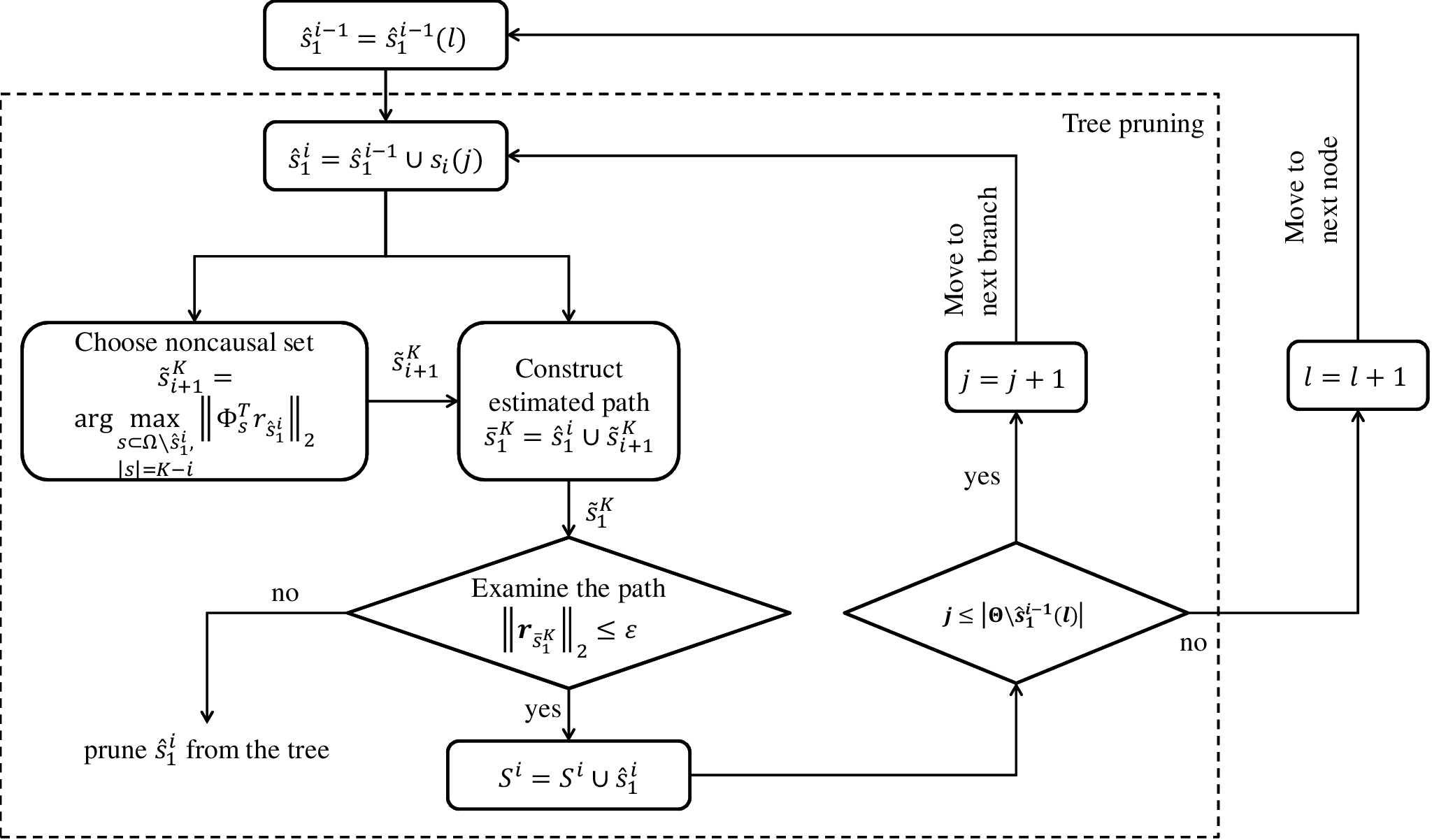
The aim of this paper is to introduce an efficient tree search algorithm to recover the sparse signal referred to as the matching pursuit with a tree pruning (TMP). Our approach significantly reduces the computational burden of the exhaustive search yet achieves excellent recovery performance in both noiseless and noisy scenarios. Two key ingredients of the TMP algorithm accomplishing this mission are the pre-selection to put a restriction on columns of 𝚽\mathbf{\Phi} to be investigated and the tree pruning to eliminate unpromising paths from the search tree. In the pre-selection stage, we choose a small number of promising columns in the sensing matrix using a conventional greedy algorithm. If we denote the set of column indices obtained in the pre-selection stage as Θ\Theta, then we set N≫|Θ|>KN\gg|\Theta|>K where KK is the sparsity of the input vector (‖𝐱‖0=K\|\mathbf{x}\|_{0}=K). When we construct the tree for the search, we only use elements of Θ\Theta as a child node in the branching process so that relentless growth of the tree can be prevented. In our empirical results, we show that TMP achieves near best performance only with |Θ|≈2​K|\Theta|\approx 2K. Once the pre-selection is finished, a tree search is performed to find best estimate of support using the pre-selected set Θ\Theta. As mentioned, when we select the child node (new estimate of the support element), we only consider the elements of Θ\Theta. As a result, the number of all possible paths in the tree is reduced from (NK)\binom{N}{K} to (|Θ|K)\binom{|\Theta|}{K}. While this reduction is phenomenal, searching all of these is still computationally demanding, in particular for large NN and nontrivial KK. In order to alleviate computational burden and at the same time maintain the effectiveness of the search, we introduce an aggressive tree pruning strategy by which unpromising paths are removed from the tree. Note that to perform the tree pruning, we need to compare the cost function J⁡(Λ)=‖𝐲−𝚽Λ​𝐱^Λ‖2J(\Lambda)=\|\mathbf{y}-\mathbf{\Phi}_{\Lambda}\hat{\mathbf{x}}_{\Lambda}\|_{2} of the full-blown candidate Λ\Lambda (‖Λ‖0=K\|\Lambda\|_{0}=K) against a pruning threshold. However, direct evaluation of J⁡(Λ)J(\Lambda) is not possible in the middle of search due to the causality of the search process so that we combine already selected indices (henceforth dubbed as the causal set) and roughly estimated indices (noncausal set). If this roughly estimated cost function is greater than the deliberately designed pruning threshold ϵ\epsilon (i.e., J⁡(Λ)>ϵJ(\Lambda)>\epsilon), further investigation of the path is hopeless and hence we prune the path from the tree immediately.

In our analysis, we show that the proposed method can accurately identify the support of KK-sparse signal and hence reconstruct the original sparse signal accurately in the noiseless setting if the sensing matrix satisfies the property so called restricted isometry property (RIP) (Theorem III.9). In the noisy setting, we show that the accurate identification of support is possible if the signal power is sufficiently larger than the noise power (Theorem III.18). In our empirical simulations, we confirm that TMP performs close to an ideal estimator11 1 The estimator that has a prior knowledge on the support (which component of the sparse vector is zero or not) is often called Oracle estimator. (often called Oracle estimator [15]) in the high SNR regime.

The rest of this paper is organized as follows. In Section II, we introduce the proposed TMP algorithm. In Section III, we analyze the recovery condition under which TMP identifies the support accurately in the noiseless and noisy scenarios. In Section IV, we provide the empirical results and then conclude the paper in Section V.

TABLE I: The TMP algorithm
Input: measurement 𝐲\mathbf{y}, sensing matrix 𝚽\mathbf{\Phi}, sparsity KK, initial threshold ϵ1\epsilon_{1}
Output: Estimated signal 𝐱^\hat{\mathbf{x}}
Initialization: i:=0i:=0, S0:=∅S^{0}:=\emptyset
Θ=fpreselection​(𝐲,𝚽,p)\Theta=f_{\text{preselection}}\left(\mathbf{y},\,\mathbf{\Phi},\,p\right) (preselection)
while i<Ki<K do
    i:=i+1i:=i+1, Si:=∅S^{i}:=\emptyset, ϵi+1:=ϵi\epsilon_{i+1}:=\epsilon_{i}
    for l=1l=1 to |Si−1||S^{i-1}| do
     θ:=Θ∖s^1i−1​(l)\theta:=\Theta\setminus\hat{s}_{1}^{i-1}(l)
     for j=1j=1 to |θ||\theta| do
      s^1i:=s^1i−1​(l)∪{si​(j)}\hat{s}_{1}^{i}:=\hat{s}_{1}^{i-1}(l)\cup\left\{s_{i}(j)\right\} (update jj-th path)
      if s^1i∉Si\hat{s}_{1}^{i}\not\in S^{i} then (check the duplicated path)
      s~i+1K=argmaxs⊂Ω,|s|=K−i∥𝚽s′𝐫s^1i∥2\tilde{s}_{i+1}^{K}\!=\!\arg\!\mathop{\max}\limits_{\mathop{s\subset\Omega,}\limits_{|s|=K-i}}\!\|\mathbf{\Phi}_{s}^{\prime}\!\mathbf{r}_{\hat{s}_{1}^{i}}\!\!\|_{2} (support estimation)
       s¯1K=s^1i∪s~i+1K\bar{s}_{1}^{K}=\hat{s}_{1}^{i}\cup\tilde{s}_{i+1}^{K}, 𝐫s¯1K=𝐏s¯1K⊥​𝐲\mathbf{r}_{\bar{s}_{1}^{K}}=\mathbf{P}_{\bar{s}_{1}^{K}}^{\bot}\mathbf{y}
      if ‖𝐫s¯1K‖2≤ϵi\|\mathbf{r}_{\bar{s}_{1}^{K}}\|_{2}\leq\epsilon_{i} then (pruning decision)
        Si:=Si∪s^1iS^{i}:=S^{i}\cup\hat{s}_{1}^{i}, I∗:=s¯1KI^{*}:=\bar{s}_{1}^{K}
        if ‖𝐫I∗‖2≤ϵi+1\|\mathbf{r}_{I^{*}}\|_{2}\leq\epsilon_{i+1} then
       ϵi+1:=‖𝐫I∗‖2\epsilon_{i+1}:=\left\|\mathbf{r}_{I^{*}}\right\|_{2} (update pruning threshold)
        end if
       end if
       end if
      end for
     end for
end while
return 𝐱^∗=𝚽I∗†​𝐲\hat{\mathbf{x}}^{*}=\mathbf{\Phi}^{\dagger}_{I^{*}}\mathbf{y} (signal reconstruction)

The fpreselection​(⋅)f_{\text{preselection}}(\cdot) is a function to choose multiple promising indices (see Section II.A).

II Matching pursuit with a tree pruning

The proposed TMP algorithm consists of two steps: pre-selection and tree search. We first describe the pre-selection process and then discuss the efficient greedy tree search.

II-A Pre-selection: A First Stage Pruning

The purpose of the pre-selection is to estimate indices that are highly likely to be the elements of support TT. Alternatively put, we do our best guess to choose columns of sensing matrix that are associated with nonzero elements of the sparse vector. Denoting the set of indices as Θ\Theta, then the search set is reduced from Ω={1,2,⋯,N}\Omega=\{1,2,\cdots,N\} to Θ\Theta, a small subset of Ω\Omega. When we perform the tree search, we only use elements of the pre-selected set Θ\Theta as a new element in the child paths so that we can limit the number of paths in the tree and eventually reduce the search complexity. In the construction of Θ\Theta, one can basically use any sparse recovery algorithm returning more than KK indices. Well-known examples include the OMP algorithm running more than K-iterations [16] or the generalized OMP algorithm [17].

II-B Tree Search with Pruning

Once the pre-selection is finished, we perform the tree search to identify the support. In this setting, the tree has a maximum depth KK, and the goal is to find a path with depth KK (i.e., candidate with cardinality KK) that has the smallest cost function J⁡(Λ)=‖𝐲−𝚽Λ​𝐱^Λ‖2J(\Lambda)=\|\mathbf{y}-\mathbf{\Phi}_{\Lambda}\hat{\mathbf{x}}_{\Lambda}\|_{2}. This cost function is often referred to as ℓ2\ell_{2}-norm of the residual 𝐫Λ=𝐲−𝚽Λ​𝐱^Λ\mathbf{r}_{\Lambda}=\mathbf{y}-\mathbf{\Phi}_{\Lambda}\hat{\mathbf{x}}_{\Lambda}. In each iteration, new child path is generated by adding new element to the existing path. If we denote the path22 2 In this paper, we use path and candidate interchangeably. In particular, we denote a full-blown path s¯1K\bar{s}_{1}^{K} by candidate. at layer (iteration) ii as s^1i\hat{s}_{1}^{i}, then s^1i={s1,s2,⋯si}\hat{s}_{1}^{i}=\{s_{1},s_{2},\cdots s_{i}\} is the causal set chosen in the first ii iterations. Since visiting all possible child nodes to find out the optimal solution is clearly prohibitive, we introduce an aggressive pruning strategy to remove unpromising paths from the tree. This pruning decision is done by comparing the cost function of the path and the pruning threshold chosen by the smallest cost function of all paths visited.

Refer to caption
Fig. 2: The pruning operation of TMP in the ii-th layer where jj is the index of column in Θ∖s^1i−1\Theta\setminus\hat{s}_{1}^{i-1}. Note that TMP investigates each path s^1i\hat{s}_{1}^{i} and performs the pruning of the path if ‖𝐫s^1i∪s~i+1K‖2>ϵ\|\mathbf{r}_{\hat{s}_{1}^{i}\cup\tilde{s}_{i+1}^{K}}\|_{2}>\epsilon.

It is worth mentioning that in contrast to typical tree search problems, it is not easy, and in fact not possible, to decide the pruning of a path using the causal set only. We note that in many tree search problems, the cost function of the path increases monotonically with the iteration (e.g., Viterbi decoding algorithm for maximum-likelihood detection) [18, 19, 20]. Therefore, if a path whose partial cost function generated by the contributions of causal path only exceeds the cost function of already visited full-blown path, the path under investigation cannot be the solution of the problem and hence can be pruned immediately from the tree (see Fig. 3).

Refer to caption
Fig. 3: Cost function of the path: (a) conventional tree search and (b) proposed tree search.

This pruning strategy, unfortunately, cannot be applied to the problem at hand since the partial cost function, which corresponds to the magnitude of the residual, is a monotonic decreasing function of the iteration33 3 If s^1i⊂s^1i+1\hat{s}_{1}^{i}\subset\hat{s}_{1}^{i+1}, then ‖𝐫s^1i‖2≥‖𝐫s^1i+1‖2\|\mathbf{r}_{\hat{s}_{1}^{i}}\|_{2}\geq\|\mathbf{r}_{\hat{s}_{1}^{i+1}}\|_{2}.. To make a proper decision, therefore, we have no way but to consider the cost function of full-blown path and hence need a noncausal set s~i+1K={si+1,si+2,⋯,sK}\tilde{s}_{i+1}^{K}=\{s_{i+1},\,s_{i+2},\,\cdots,\,s_{K}\} in the pruning process. This noncausal set s~i+1K\tilde{s}_{i+1}^{K} is temporarily needed for the pruning operation and can be easily obtained by choosing K−iK-i indices of columns in Ω∖s^1i\Omega\setminus\hat{s}_{1}^{i} whose magnitude of the correlation with the residual 𝐫s^1i\mathbf{r}_{\hat{s}_{1}^{i}} is maximal44 4 Instead of a single-shot process choosing K−iK-i indices simultaneously, noncausal set s~i+1K\tilde{s}_{i+1}^{K} can be chosen by running multiple iterations for better judgement.. That is,

s~i+1K=argmaxs⊂Ω∖s^1i,|s|=K−i‖𝚽s′𝐫s^1i‖2\displaystyle\tilde{s}_{i+1}^{K}=\arg\mathop{\max_{s\subset\Omega\setminus\hat{s}_{1}^{i},}}\limits_{|s|=K-i}\left\|\mathbf{\Phi}_{s}^{\prime}\mathbf{r}_{\hat{s}_{1}^{i}}\right\|_{2} (2)

where

𝐫s^1i\displaystyle\mathbf{r}_{\hat{s}_{1}^{i}} =\displaystyle= 𝐲−𝚽s^1i​𝐱^s^1i,\displaystyle\mathbf{y}-\mathbf{\Phi}_{\hat{s}_{1}^{i}}\hat{\mathbf{x}}_{\hat{s}_{1}^{i}},
𝐱^s^1i\displaystyle\hat{\mathbf{x}}_{\hat{s}_{1}^{i}} =\displaystyle= 𝚽s^1i†​𝐲.\displaystyle\mathbf{\Phi}^{\dagger}_{\hat{s}_{1}^{i}}\mathbf{y}.

For example, if K−i=2K-i=2, Ω∖s^1i={5,7,9,11,⋯}\Omega\setminus\hat{s}_{1}^{i}=\{5,7,9,11,\cdots\}, and

|ϕ7′​𝐫s^1i|>|ϕ11′​𝐫s^1i|>|ϕ5′​𝐫s^1i|>|ϕ9′​𝐫s^1i|>⋯,|\mathbf{\phi}_{7}^{\prime}\mathbf{r}_{\hat{s}_{1}^{i}}|>|\mathbf{\phi}_{11}^{\prime}\mathbf{r}_{\hat{s}_{1}^{i}}|>|\mathbf{\phi}_{5}^{\prime}\mathbf{r}_{\hat{s}_{1}^{i}}|>|\mathbf{\phi}_{9}^{\prime}\mathbf{r}_{\hat{s}_{1}^{i}}|>\cdots,

then the noncausal set is s~i+1K={7,11}\tilde{s}_{i+1}^{K}=\{7,11\}.

Once roughly estimated candidate s¯1K=s^1i∪s~i+1K\bar{s}_{1}^{K}=\hat{s}_{1}^{i}\cup\tilde{s}_{i+1}^{K} is obtained, we compute the residual 𝐫s¯1K=𝐲−𝚽s¯1K​𝐱^s¯1K\mathbf{r}_{\bar{s}_{1}^{K}}=\mathbf{y}-\mathbf{\Phi}_{\bar{s}_{1}^{K}}\hat{\mathbf{x}}_{\bar{s}_{1}^{K}} (𝐱^s¯1K=𝚽s¯1K†​𝐲\hat{\mathbf{x}}_{\bar{s}_{1}^{K}}=\mathbf{\Phi}_{\bar{s}_{1}^{K}}^{\dagger}\mathbf{y}) to decide whether to prune this path or not. To be specific, if the ℓ2\ell_{2}-norm of the residual is greater than the threshold ϵ\epsilon (i.e., ‖𝐫s¯1K‖2>ϵ\|\mathbf{r}_{\bar{s}_{1}^{K}}\|_{2}>\epsilon), then the path has little hope to survive and hence is pruned immediately (see Fig. 1). Note that the pruning threshold ϵ\epsilon is initialized to a large number and whenever the search of a layer is finished, updated to the minimum ℓ2\ell_{2}-norm of the residual among all survived paths (ϵ=min⁡‖𝐫s¯1K‖2\epsilon=\min\|\mathbf{r}_{\bar{s}_{1}^{K}}\|_{2}). Once the search is finished, a path with the minimum cost function is chosen as the final output of TMP. We summarize the proposed TMP algorithm in Table I.

III Performance Analysis

In this section, we analyze the recovery conditions under which TMP can accurately identify KK-sparse signals in noiseless and noisy scenarios. In our analysis, we use the restricted isometry property (RIP) of the sensing matrix.

Definition III.1

The sensing matrix 𝚽\mathbf{\Phi} is said to satisfy the RIP of order KK if there exists a constant δ⁡(𝚽)∈(0,1)\delta(\mathbf{\Phi})\in(0,1) such that

(1−δ⁡(𝚽))​‖𝐱‖22≤‖𝚽​𝐱‖22≤(1+δ⁡(𝚽))​‖𝐱‖22(1-\delta(\mathbf{\Phi}))\|\mathbf{x}\|_{2}^{2}\leq\|\mathbf{\Phi}\mathbf{x}\|_{2}^{2}\leq(1+\delta(\mathbf{\Phi}))\|\mathbf{x}\|_{2}^{2}

for any KK-sparse vector 𝐱\mathbf{x}.

In particular, the minimum of all constants δ⁡(𝚽)\delta(\mathbf{\Phi}) satisfying Definition III.1 is called the restricted isometry constant (RIC) and denoted by δK​(𝚽)\delta_{K}(\mathbf{\Phi}). In the sequel, we use δK\delta_{K} instead of δK​(𝚽)\delta_{K}(\mathbf{\Phi}) for brevity.

In our analysis, we use the generalized OMP (gOMP) as a pre-selection algorithm. The gOMP algorithm chooses LL (>1>1) indices in each iteration and hence L​KLK indices are chosen in total. Due to the selection of multiple indices, more than one true indices (indices in the support) can be chosen in each iteration and the chance of identifying the support increases substantially [17].

The following lemmas are useful in our analysis.

Lemma III.2

(Lemma 3 in [2]): If the sensing matrix 𝚽\mathbf{\Phi} satisfies the RIP of both orders K1K_{1} and K2K_{2}, then δK1<δK2\delta_{K_{1}}<\delta_{K_{2}} for any K1<K2K_{1}<K_{2}.

Lemma III.3

(Consequences of RIP [2, 9]): If 0<δ|I|<10<\delta_{|I|}<1 exists for I⊂ΩI\subset\Omega, then for any vector 𝐱∈ℝ|I|\mathbf{x}\in\mathbb{R}^{|I|},

(1−δ|I|)​‖𝐱‖2≤‖𝚽I′​𝚽I​𝐱‖2≤(1+δ|I|)​‖𝐱‖2,\displaystyle\left(1-\delta_{|I|}\right)\|\mathbf{x}\|_{2}\leq\|\mathbf{\Phi}_{I}^{\prime}\mathbf{\Phi}_{I}\mathbf{x}\|_{2}\leq\left(1+\delta_{|I|}\right)\|\mathbf{x}\|_{2},
11+δ|I|​‖𝐱‖2≤‖(𝚽I′​𝚽I)−1​𝐱‖2≤11−δ|I|​‖𝐱‖2.\displaystyle\frac{1}{1+\delta_{|I|}}\|\mathbf{x}\|_{2}\leq\|\left(\mathbf{\Phi}_{I}^{\prime}\mathbf{\Phi}_{I}\right)^{-1}\mathbf{x}\|_{2}\leq\frac{1}{1-\delta_{|I|}}\|\mathbf{x}\|_{2}.
Lemma III.4

(Lemma 2.1 in [4]): Let I1,I2⊂ΩI_{1},\,I_{2}\subset\Omega and I1∩I2=∅I_{1}\cap I_{2}=\emptyset. If 0<δ|I1|+|I2|<10<\delta_{|I_{1}|+|I_{2}|}<1 exists, then

‖𝚽I1′​𝚽I2​𝐱‖2≤δ|I1|+|I2|​‖𝐱‖2.\displaystyle\|\mathbf{\Phi}_{I_{1}}^{\prime}\mathbf{\Phi}_{I_{2}}\mathbf{x}\|_{2}\leq\delta_{|I_{1}|+|I_{2}|}\|\mathbf{x}\|_{2}.

III-A Recovery from Noiseless Measurements

In this subsection, we analyze a condition ensuring that TMP recovers the original sparse signal accurately from the noiseless measurements. As mentioned, TMP consists of pre-selection and tree search. In our analysis, we show that the recovery condition of TMP is not much different from the condition of the pre-selection only and in fact guaranteed under more relaxed RIP bound (see Theorem III.9).

In order to ensure the accurate identification of the support, TMP should satisfy the following two conditions:

  1. 1.

    At least one support index should be selected in the pre-selection process (i.e., T∩Θ≠∅T\cap\Theta\neq\emptyset).

  2. 2.

    At least one true path55 5 If s^1i\hat{s}_{1}^{i} is a true path, it contains indices only in TT (s^1i⊂T\hat{s}_{1}^{i}\subset T). should be survived in the tree pruning process.

The following Theorem describes the condition ensuring that at least one support is identified by the pre-selection stage.

Theorem III.5 (Recovery condition in first iteration for noiseless scenario [17])

The gOMP algorithm identifies at least one support index in the first iteration if the sensing matrix 𝚽\mathbf{\Phi} satisfies

δL+K<LL+K.\delta_{L+K}<\frac{\sqrt{L}}{\sqrt{L}+\sqrt{K}}. (3)

We next analyze the condition ensuring that the final candidate s¯1K\bar{s}_{1}^{K} of the tree search equals the support TT. In order to guarantee s¯1K=T\bar{s}_{1}^{K}=T, at least one true path should be survived in each layer and further a true index should be added to this path.

Before we proceed, we provide definitions useful in our analysis. Let λi\lambda_{i} be the smallest correlation in magnitude between the residual 𝐫s^1i\mathbf{r}_{\hat{s}_{1}^{i}} and columns associated with correct indices. That is,

λi=minu∈T∖s^1i|ϕu′​𝐫s^1i|.\lambda^{i}=\mathop{\min}\limits_{u\in T\setminus\hat{s}_{1}^{i}}\left|\phi_{u}^{\prime}\mathbf{r}_{\hat{s}_{1}^{i}}\right|.

Further, let γi\gamma^{i} be the largest correlation in magnitude between 𝐫s^1i\mathbf{r}_{\hat{s}_{1}^{i}} and columns associated with incorrect indices. That is,

γi=maxu∈Tc|<ϕu,𝐫s^1i>|.\gamma^{i}=\mathop{\max}\limits_{u\in T^{c}}\left|<\phi_{u},\mathbf{r}_{\hat{s}_{1}^{i}}>\right|.

In the following lemmas, we provide a lower bound of λi\lambda^{i} and an upper bound of γi\gamma^{i}.

Lemma III.6

Suppose a path s^1i\hat{s}_{1}^{i} is contained in TT (i.e., s^1i⊂T\hat{s}_{1}^{i}\subset T), then

λi≥1−δK−δM1−δK​‖𝐱T∖s^1i‖2.\lambda^{i}\geq\frac{1-\delta_{K}-\delta_{M}}{1-\delta_{K}}\left\|\mathbf{x}_{T\setminus\hat{s}_{1}^{i}}\right\|_{2}. (4)
Proof:

See Appendix A. ∎

Lemma III.7

Suppose a path s^1i\hat{s}_{1}^{i} is contained in TT, then

γi≤δK+11−δK​‖𝐱T∖s^1i‖2.\gamma^{i}\leq\frac{\delta_{K+1}}{1-\delta_{K}}\left\|\mathbf{x}_{T\setminus\hat{s}_{1}^{i}}\right\|_{2}. (5)
Proof:

See Appendix B. ∎

As mentioned, in order to recover the original sparse signals, at least one true path should be survived in each layer. In other words, when a path s^1i\hat{s}_{1}^{i} is contained in TT (s^1i⊂T\hat{s}_{1}^{i}\subset T), then the noncausal set s~i+1K\tilde{s}_{i+1}^{K} should also be contained in TT (i.e., s~i+1K⊂T\tilde{s}_{i+1}^{K}\subset T) and further this path should not be pruned for the accurate reconstruction of the sparse signals. That is,

‖𝐫s^1i∪s~i+1K‖=‖𝐫T‖<ϵ.\|\mathbf{r}_{\hat{s}_{1}^{i}\cup\tilde{s}_{i+1}^{K}}\|=\|\mathbf{r}_{T}\|<\epsilon. (6)

Since ‖𝐫T‖2=0\|\mathbf{r}_{T}\|_{2}=0 for the noiseless scenario, the condition (6) always holds for any positive ϵ\epsilon. Thus, what we essentially need is a condition ensuring that the noncausal set chosen from (2) is contained in TT (i.e., s~i+1K⊂T\tilde{s}_{i+1}^{K}\subset T).

Refer to caption
Fig. 4: Comparison between λi\lambda^{i} and γi\gamma^{i} for the true path s^1i\hat{s}_{1}^{i} (i.e., s^1i⊂T\hat{s}_{1}^{i}\subset T). λi\lambda_{i} is the smallest correlation (in magnitude) between the residual 𝐫s^1i\mathbf{r}_{\hat{s}_{1}^{i}} and columns associated with T∖s^1iT\setminus\hat{s}_{1}^{i} and γi\gamma^{i} is the largest correlation (in magnitude) between 𝐫s^1i\mathbf{r}_{\hat{s}_{1}^{i}} and columns associated with TcT^{c}. One can observe that, if λi>γi\lambda^{i}>\gamma^{i}, then the noncausal set s¯1K\bar{s}_{1}^{K} is contained in TT (s¯1K=T∖s^1i\bar{s}_{1}^{K}=T\setminus\hat{s}_{1}^{i}).
Theorem III.8

If the causal path s^1i\hat{s}_{1}^{i} contains correct indices only, then the noncausal set s~i+1K\tilde{s}_{i+1}^{K} of TMP consist only of correct ones under

δM<13.\delta_{M}<\frac{1}{3}. (7)

for any ii (0≤i≤K−10\leq i\leq K-1). In other words, s¯1K(=s^1i∪s~i+1K)=T\bar{s}_{1}^{K}(=\hat{s}_{1}^{i}\cup\tilde{s}_{i+1}^{K})=T under δM<13\delta_{M}<\frac{1}{3}.

Proof:

Since the indices of columns highly correlated with 𝐫s^1i\mathbf{r}_{\hat{s}_{1}^{i}} are chosen as elements of s~i+1K\tilde{s}_{i+1}^{K} (see (2)), if λi\lambda^{i} is larger than γi\gamma^{i}, then the noncausal set s~i+1K\tilde{s}_{i+1}^{K} is contained in TT (s~i+1K=T∖s^1i\tilde{s}_{i+1}^{K}=T\setminus\hat{s}_{1}^{i}). In other words, s¯1K=T\bar{s}_{1}^{K}=T under

λi>γi.\lambda^{i}>\gamma^{i}. (8)

Using Lemma III.6 and III.7, (8) holds under 1 - δ K - δ M 1-δ K ‖ x_T ∖ ^ s _1^i ‖_2 ¿ δ K+1 1-δ K ‖ x_T∖ ^ s _1^i ‖_2, and hence δK+δK+1+δM<1\delta_{K}+\delta_{K+1}+\delta_{M}<1. Further, using Lemma III.2, we have 3​δM<13\delta_{M}<1, which is the desired result. ∎

If Theorem III.5 and III.8 are jointly satisfied, s~i+1K⊂T\tilde{s}_{i+1}^{K}\subset T for any true path s^1i\hat{s}_{1}^{i} (s^1i⊂T\hat{s}_{1}^{i}\subset T) so that s¯1K=s^1i∪s~i+1K=T\bar{s}_{1}^{K}=\hat{s}_{1}^{i}\cup\tilde{s}_{i+1}^{K}=T and thus s^1i\hat{s}_{1}^{i} will not be pruned from the tree (we recall that ‖𝐫s¯1K‖2=0<ϵ\|\mathbf{r}_{\bar{s}_{1}^{K}}\|_{2}=0<\epsilon for any positive ϵ\epsilon). Therefore, overall recovery condition of TMP for the noiseless scenario can be obtained by combining Theorem III.5 and III.8.

Theorem III.9 (Recovery condition of TMP)

The TMP algorithm identifies the support of any KK-sparse signal from 𝐲=𝚽​𝐱\mathbf{y}=\mathbf{\Phi x} accurately if the sensing matrix 𝚽\mathbf{\Phi} satisfies the RIP with

δQ<13\displaystyle\delta_{Q}<\frac{1}{3} if ​K<4​L,\displaystyle\text{if }K<4L, (9)
δQ<LL+K\displaystyle\delta_{Q}<\frac{\sqrt{L}}{\sqrt{L}+\sqrt{K}} otherwise (10)

where Q=max⁡{M,L+K}Q=\max\{M,L+K\}.

Proof:

The conditions (9) and (10) are obtained by choosing stricter condition between Theorem III.5 and III.8. Specifically,

if ​LL+K>13\displaystyle\text{if }\frac{\sqrt{L}}{\sqrt{L}+\sqrt{K}}>\frac{1}{3} →\displaystyle\rightarrow δQ<13\displaystyle\delta_{Q}<\frac{1}{3}
otherwise →\displaystyle\rightarrow δQ<LL+K,\displaystyle\delta_{Q}<\frac{\sqrt{L}}{\sqrt{L}+\sqrt{K}},

which is the desired result. ∎

Recall that the exact recovery condition of the original gOMP algorithm is [17]

δL​K<LL+2​K.\displaystyle\delta_{LK}<\frac{\sqrt{L}}{\sqrt{L}+2\sqrt{K}}. (11)

From (9)-(11), it is clear that TMP provides more relaxed upper bound for any L<KL<K since LL+2​K<min⁡{13,LL+K}\frac{\sqrt{L}}{\sqrt{L}+2\sqrt{K}}<\min\{\frac{1}{3},\,\frac{\sqrt{L}}{\sqrt{L}+\sqrt{K}}\}. Even if L=KL=K, TMP is effective since the exact recovery conditions of gOMP and TMP are

δK2<13\delta_{K^{2}}<\frac{1}{3}

and

δmax⁡{M,2​K}<13,\delta_{\max\{M,2K\}}<\frac{1}{3},

respectively. One can observe that in the large dimensional system satisfying K2>MK^{2}>M, recovery condition of TMP is better (more relaxed) than the condition of gOMP. Similar argument holds for other sparse recovery algorithm (e.g., CoSaMP [9]).

III-B Reconstruction from Noisy Measurements

Now, we turn to the noisy scenario and analyze the condition of TMP to accurately identify the support in the presence of noise. Even though the details are a bit cumbersome, main architecture of the proof is reminiscent of the argument in the noiseless scenario. In fact, two requirements of TMP to identify the support are 1) at least one support element should be chosen in the pre-selection process (i.e., T∩Ω≠∅T\cap\Omega\neq\emptyset), and 2) true path (s¯1K=T\bar{s}_{1}^{K}=T) should be survived in the pruning process.

Before we proceed, we provide useful definitions in our analysis. First, let ρ\rho be the largest correlation (in magnitude) between the observation 𝐲\mathbf{y} and the columns associated with true indices. That is,

ρ=maxj∈T⁡|ϕj′​𝐲|.\displaystyle\rho=\max_{j\in T}|\phi_{j}^{\prime}\mathbf{y}|.

Next, let η\eta be the LL-th largest correlation (in magnitude) between the observation 𝐲\mathbf{y} and the columns associated with incorrect indices. Then η\eta is expressed as

η=minj∈IL⁡|ϕj′​𝐲|.\displaystyle\eta=\min_{j\in I_{L}}|\phi_{j}^{\prime}\mathbf{y}|.

where IL=argmax|I|=L,I⊂Tc∥𝚽I′𝐫Λ∥2I_{L}=\arg\mathop{\max}\limits_{|I|=L,I\subset T^{c}}\|\mathbf{\Phi}_{I}^{\prime}\mathbf{r}_{\Lambda}\|_{2}.

In the following lemmas, we provide the lower bound of ρ\rho and the upper bound of η\eta.

Lemma III.10

ρ\rho satisfies

ρ≥1K​[(1−δK)​‖𝐱T‖2−1+δK​‖𝐯‖2]\displaystyle\rho\geq\frac{1}{\sqrt{K}}\left[\left(1-\delta_{K}\right)\|\mathbf{x}_{T}\|_{2}-\sqrt{1+\delta_{K}}\|\mathbf{v}\|_{2}\right] (12)
Proof:

See Appendex C. ∎

Lemma III.11

η\eta satisfies

η≤1L​[δL+K​‖𝐱T‖2+1+δL​‖𝐯‖2].\displaystyle\eta\leq\frac{1}{\sqrt{L}}\left[\delta_{L+K}\|\mathbf{x}_{T}\|_{2}+\sqrt{1+\delta_{L}}\|\mathbf{v}\|_{2}\right]. (13)
Proof:

See Appendex D. ∎

The following theorem provides the condition ensuring that at least one support element is identified by the pre-selection stage.

Theorem III.12

The gOMP algorithm identifies at least one support element if the nonzero coefficients of the original sparse signal 𝐱\mathbf{x} satisfy

minj∈T⁡|xj|>(K+L)​1+δL+KL​(1−δK)−K​δL+K​‖𝐯‖2.\displaystyle\min_{j\in T}|x_{j}|>\frac{(\sqrt{K}+\sqrt{L})\sqrt{1+\delta_{L+K}}}{\sqrt{L}(1-\delta_{K})-\sqrt{K}\delta_{L+K}}\|\mathbf{v}\|_{2}. (14)
Proof:

From definitions of ρ\rho and η\eta, it is clear that gOMP selects at least one true index in the first iteration if

ρ>η.\displaystyle\rho>\eta. (15)

Using the lower bound of ρ\rho and the upper bound of η\eta, we obtain the sufficient condition of (15) as

1K​[(1−δK)​‖𝐱T‖2−1+δK​‖𝐯‖2]>1L​[δL+K​‖𝐱T‖2+1+δL​‖𝐯‖2].\displaystyle\frac{1}{\sqrt{K}}\left[\left(1-\delta_{K}\right)\|\mathbf{x}_{T}\|_{2}-\sqrt{1+\delta_{K}}\|\mathbf{v}\|_{2}\right]>\frac{1}{\sqrt{L}}\left[\delta_{L+K}\|\mathbf{x}_{T}\|_{2}+\sqrt{1+\delta_{L}}\|\mathbf{v}\|_{2}\right]. (16)

After some manipulations, we have

‖𝐱T‖2>(K+L)​1+δL+KL​(1−δK)−K​δL+K​‖𝐯‖2.\displaystyle\|\mathbf{x}_{T}\|_{2}>\frac{(\sqrt{K}+\sqrt{L})\sqrt{1+\delta_{L+K}}}{\sqrt{L}(1-\delta_{K})-\sqrt{K}\delta_{L+K}}\|\mathbf{v}\|_{2}. (17)

Since ‖𝐱T‖2≥minj∈T|xj|\|\mathbf{x}_{T}\|_{2}\geq\mathop{\min}\limits_{j\in T}|x_{j}|, (17) is guaranteed under

minj∈T⁡|xj|>(K+L)​1+δL+KL​(1−δK)−K​δL+K​‖𝐯‖2,\displaystyle\min_{j\in T}|x_{j}|>\frac{(\sqrt{K}+\sqrt{L})\sqrt{1+\delta_{L+K}}}{\sqrt{L}(1-\delta_{K})-\sqrt{K}\delta_{L+K}}\|\mathbf{v}\|_{2}, (18)

which completes the proof. ∎

We next analyze the condition under which the true path is survived by the tree pruning stage. In order to meet this requirement, 1) under the condition that a causal set is true (s^1i⊂T\hat{s}_{1}^{i}\subset T), corresponding noncausal set should also be true (s~i+1K⊂T\tilde{s}_{i+1}^{K}\subset T) and further 2) this true path should not be removed by the tree pruning (i.e., if s¯1K=T\bar{s}_{1}^{K}=T, then ‖𝐫s¯1K‖2<ϵ\|\mathbf{r}_{\bar{s}_{1}^{K}}\|_{2}<\epsilon).

Before we proceed, we introduce two useful definitions in our analysis. Let βi\beta^{i} be the smallest correlation in magnitude between ϕj\phi_{j} (j∈T∖s^1ij\in T\setminus\hat{s}_{1}^{i}) and 𝐫s^1i\mathbf{r}_{\hat{s}_{1}^{i}}:

βi=arg⁡minj∈T∖s^1i​|ϕj′​𝐫s^1i|.\displaystyle\beta^{i}=\arg\min_{j\in T\setminus\hat{s}_{1}^{i}}|\phi_{j}^{\prime}\mathbf{r}_{\hat{s}_{1}^{i}}|.

Similarly, let αi\alpha^{i} be the largest correlation in magnitude between ϕj\phi_{j} (j∈Tcj\in T^{c}) and the residual 𝐫s^1i\mathbf{r}_{\hat{s}_{1}^{i}}:

αi=arg⁡maxj∈Tc​|ϕj′​𝐫s^1i|.\displaystyle\alpha^{i}=\arg\max_{j\in T^{c}}|\phi_{j}^{\prime}\mathbf{r}_{\hat{s}_{1}^{i}}|.

The following two lemmas provide the lower and upper bounds of βi\beta^{i} and αi\alpha^{i}, respectively.

Lemma III.13

If s^1i\hat{s}_{1}^{i} contains true indices exclusively, then βi\beta^{i} satisfies

βi≥(1−δM−δK+1​δK1−δK)​‖𝐱T∖s^1i‖2−1+δM​‖𝐯‖2\displaystyle\beta^{i}\geq\left(1-\delta_{M}-\frac{\delta_{K+1}\delta_{K}}{1-\delta_{K}}\right)\|\mathbf{x}_{T\setminus\hat{s}_{1}^{i}}\|_{2}-\sqrt{1+\delta_{M}}\|\mathbf{v}\|_{2} (19)
Proof:

See Appendix E. ∎

Lemma III.14

If s^1i\hat{s}_{1}^{i} contains true indices exclusively, then αi\alpha^{i} satisfies

αi≤(δK+1+δK+1​δK1−δK)​‖𝐱T∖s^1i‖2+1+δM​‖𝐯‖2\displaystyle\alpha^{i}\leq\left(\delta_{K+1}+\frac{\delta_{K+1}\delta_{K}}{1-\delta_{K}}\right)\|\mathbf{x}_{T\setminus\hat{s}_{1}^{i}}\|_{2}+\sqrt{1+\delta_{M}}\|\mathbf{v}\|_{2} (20)
Proof:

See Appendix F. ∎

Using these lemmas, we can identify the condition guaranteeing that the noncausal set s~i+1K\tilde{s}_{i+1}^{K} of a true path (s^1i⊂T\hat{s}_{1}^{i}\subset T) is also true.

Lemma III.15

Suppose a causal path s^1i\hat{s}_{1}^{i} consists of true indices exclusively (i.e., s^1i⊂T\hat{s}_{1}^{i}\subset T), then the noncausal set s~i+1K\tilde{s}_{i+1}^{K} also contains the true ones (s~i+1K=T∖s^1i\tilde{s}_{i+1}^{K}=T\setminus\hat{s}_{1}^{i}) under

minj∈T⁡|xj|>2​(1−δK)​1+δM1−δK−δK+1−δM​‖𝐯‖2.\displaystyle\min_{j\in T}|x_{j}|>\frac{2(1-\delta_{K})\sqrt{1+\delta_{M}}}{1-\delta_{K}-\delta_{K+1}-\delta_{M}}\|\mathbf{v}\|_{2}. (21)
Proof:

One can easily show that the noncausal set of any true path s^1i\hat{s}_{1}^{i} contains only true indices if

βi>αi.\displaystyle\beta^{i}>\alpha^{i}. (22)

Using Lemma III.13 and III.14, we obtain the sufficient condition of (22) as

(1−δM−δM​δK1−δK)​‖𝐱T∖s^1i‖2−1+δM​‖𝐯‖2\displaystyle\left(1-\delta_{M}-\frac{\delta_{M}\delta_{K}}{1-\delta_{K}}\right)\|\mathbf{x}_{T\setminus\hat{s}_{1}^{i}}\|_{2}-\sqrt{1+\delta_{M}}\|\mathbf{v}\|_{2} (23)
>(δK+1+δK+1​δK1−δK)​‖𝐱T∖s^1i‖2+1+δM​‖𝐯‖2.\displaystyle\hskip 85.35826pt>\left(\delta_{K+1}+\frac{\delta_{K+1}\delta_{K}}{1-\delta_{K}}\right)\|\mathbf{x}_{T\setminus\hat{s}_{1}^{i}}\|_{2}+\sqrt{1+\delta_{M}}\|\mathbf{v}\|_{2}.

After some manipulations, we have

‖𝐱T∖s^1i‖2>2​(1−δK)​1+δM1−δK−δK+1−δM​‖𝐯‖2.\displaystyle\|\mathbf{x}_{T\setminus\hat{s}_{1}^{i}}\|_{2}>\frac{2(1-\delta_{K})\sqrt{1+\delta_{M}}}{1-\delta_{K}-\delta_{K+1}-\delta_{M}}\|\mathbf{v}\|_{2}. (24)

Since ‖𝐱T∖s^1i‖2≥minj∈T|xj|\|\mathbf{x}_{T\setminus\hat{s}_{1}^{i}}\|_{2}\geq\mathop{\min}\limits_{j\in T}|x_{j}|, we get the desired result. ∎

Next, we turn to the analysis of the condition under which the magnitude of 𝐫T\mathbf{r}_{T} becomes the minimum among all combinations of KK indices.

Lemma III.16

The candidate whose residual is minimum (in magnitude) becomes the support if

minj∈T⁡|xj|>2​(1−δK)1−3​δ2​K​‖𝐯‖2.\min_{j\in T}|x_{j}|>\frac{2(1-\delta_{K})}{1-3\delta_{2K}}\|\mathbf{v}\|_{2}. (25)

In other words, ‖𝐫T‖2<‖𝐫s¯1K‖2\|\mathbf{r}_{T}\|_{2}<\|\mathbf{r}_{\bar{s}_{1}^{K}}\|_{2} for any s¯1K≠T\bar{s}_{1}^{K}\neq T under (25).

Proof:

One can notice that the hypothesis is satisfied if the upper bound of ‖𝐫T‖2\|\mathbf{r}_{T}\|_{2} is smaller than the lower bound of ‖𝐫s¯1K‖2\|\mathbf{r}_{\bar{s}_{1}^{K}}\|_{2}. First, we obtain the upper bound of ‖𝐫T‖2\|\mathbf{r}_{T}\|_{2} as

‖𝐫T‖2\displaystyle\|\mathbf{r}_{T}\|_{2} =\displaystyle= ‖𝐏T⊥​𝐲‖2\displaystyle\|\mathbf{P}_{T}^{\bot}\mathbf{y}\|_{2} (26)
=\displaystyle= ‖𝐏T⊥​(𝚽T​𝐱T+𝐯)‖2\displaystyle\|\mathbf{P}_{T}^{\bot}\left(\mathbf{\Phi}_{T}\mathbf{x}_{T}+\mathbf{v}\right)\|_{2}
=\displaystyle= ‖𝐏T⊥​𝐯‖2\displaystyle\|\mathbf{P}_{T}^{\bot}\mathbf{v}\|_{2}
≤\displaystyle\leq ‖𝐯‖2\displaystyle\|\mathbf{v}\|_{2}

where 𝐏T⊥=𝐈−𝚽T​(𝚽T′​𝚽T)−1​𝚽T′\mathbf{P}_{T}^{\bot}=\mathbf{I}-\mathbf{\Phi}_{T}\left(\mathbf{\Phi}_{T}^{\prime}\mathbf{\Phi}_{T}\right)^{-1}\mathbf{\Phi}_{T}^{\prime} is the projection onto the orthogonal complement of TT and (26) is because 𝐏T⊥​𝚽T​𝐱T=𝟎\mathbf{P}_{T}^{\bot}\mathbf{\Phi}_{T}\mathbf{x}_{T}=\mathbf{0}.

Next, we obtain the lower bound of ‖𝐫s¯1K‖2\|\mathbf{r}_{\bar{s}_{1}^{K}}\|_{2}. For any s¯1K≠T\bar{s}_{1}^{K}\neq T, we have

‖𝐫s¯1K‖2\displaystyle\|\mathbf{r}_{\bar{s}_{1}^{K}}\|_{2} =\displaystyle= ‖𝐏s¯1K⊥​𝐲‖2\displaystyle\|\mathbf{P}_{\bar{s}_{1}^{K}}^{\bot}\mathbf{y}\|_{2} (27)
=\displaystyle= ‖𝐏s¯1K⊥​(𝚽​𝐱+𝐯)‖2\displaystyle\|\mathbf{P}_{\bar{s}_{1}^{K}}^{\bot}(\mathbf{\Phi x}+\mathbf{v})\|_{2}
=\displaystyle= ‖𝐏s¯1K⊥​(𝚽s¯1K​𝐱s¯1K+𝚽T∖s¯1K​𝐱T∖s¯1K+𝐯)‖2\displaystyle\|\mathbf{P}_{\bar{s}_{1}^{K}}^{\bot}(\mathbf{\Phi}_{\bar{s}_{1}^{K}}\mathbf{x}_{\bar{s}_{1}^{K}}+\mathbf{\Phi}_{T\setminus\bar{s}_{1}^{K}}\mathbf{x}_{T\setminus\bar{s}_{1}^{K}}+\mathbf{v})\|_{2}
=\displaystyle= ‖𝐏s¯1K⊥​(𝚽T∖s¯1K​𝐱T∖s¯1K+𝐯)‖2\displaystyle\|\mathbf{P}_{\bar{s}_{1}^{K}}^{\bot}(\mathbf{\Phi}_{T\setminus\bar{s}_{1}^{K}}\mathbf{x}_{T\setminus\bar{s}_{1}^{K}}+\mathbf{v})\|_{2}
≥\displaystyle\geq ‖𝐏s¯1K⊥​𝚽T∖s¯1K​𝐱T∖s¯1K‖2−‖𝐏s¯1K⊥​𝐯‖2\displaystyle\|\mathbf{P}_{\bar{s}_{1}^{K}}^{\bot}\mathbf{\Phi}_{T\setminus\bar{s}_{1}^{K}}\mathbf{x}_{T\setminus\bar{s}_{1}^{K}}\|_{2}-\|\mathbf{P}_{\bar{s}_{1}^{K}}^{\bot}\mathbf{v}\|_{2} (28)

where the inequality in (27) is because 𝐏s¯1K⊥​𝚽s¯1K⊥​𝐱s¯1K⊥=𝟎\mathbf{P}_{\bar{s}_{1}^{K}}^{\bot}\mathbf{\Phi}_{\bar{s}_{1}^{K}}^{\bot}\mathbf{x}_{\bar{s}_{1}^{K}}^{\bot}=\mathbf{0} and the inequality in (28) is due to the triangle inequality. The first term in the right-hand side of (28) is lower bounded as

‖𝐏s¯1K⊥​𝚽T∖s¯1K​𝐱T∖s¯1K‖2\displaystyle\|\mathbf{P}_{\bar{s}_{1}^{K}}^{\bot}\mathbf{\Phi}_{T\setminus\bar{s}_{1}^{K}}\mathbf{x}_{T\setminus\bar{s}_{1}^{K}}\|_{2} =\displaystyle= ‖(𝐈−𝚽s¯1K​(𝚽s¯1K′​𝚽s¯1K)−1​𝚽s¯1K′)​𝚽T∖s¯1K​𝐱T∖s¯1K‖2\displaystyle\|(\mathbf{I}-\mathbf{\Phi}_{\bar{s}_{1}^{K}}(\mathbf{\Phi}_{\bar{s}_{1}^{K}}^{\prime}\mathbf{\Phi}_{\bar{s}_{1}^{K}})^{-1}\mathbf{\Phi}_{\bar{s}_{1}^{K}}^{\prime})\mathbf{\Phi}_{T\setminus\bar{s}_{1}^{K}}\mathbf{x}_{T\setminus\bar{s}_{1}^{K}}\|_{2} (29)
≥\displaystyle\geq ‖𝚽T∖s¯1K​𝐱T∖s¯1K‖2−‖𝚽s¯1K​(𝚽s¯1K′​𝚽s¯1K)−1​𝚽s¯1K′​𝚽T∖s¯1K​𝐱T∖s¯1K‖2\displaystyle\|\mathbf{\Phi}_{T\setminus\bar{s}_{1}^{K}}\mathbf{x}_{T\setminus\bar{s}_{1}^{K}}\|_{2}-\|\mathbf{\Phi}_{\bar{s}_{1}^{K}}(\mathbf{\Phi}_{\bar{s}_{1}^{K}}^{\prime}\mathbf{\Phi}_{\bar{s}_{1}^{K}})^{-1}\mathbf{\Phi}_{\bar{s}_{1}^{K}}^{\prime}\mathbf{\Phi}_{T\setminus\bar{s}_{1}^{K}}\mathbf{x}_{T\setminus\bar{s}_{1}^{K}}\|_{2}
≥\displaystyle\geq 1−δ|T∖s¯1K|​‖𝐱T∖s¯1K‖2\displaystyle\sqrt{1-\delta_{|T\setminus\bar{s}_{1}^{K}|}}\|\mathbf{x}_{T\setminus\bar{s}_{1}^{K}}\|_{2}
−1+δ|s¯1K|​‖(𝚽s¯1K′​𝚽s¯1K)−1​𝚽s¯1K′​𝚽T∖s¯1K​𝐱T∖s¯1K‖2\displaystyle-\sqrt{1+\delta_{|\bar{s}_{1}^{K}|}}\|(\mathbf{\Phi}_{\bar{s}_{1}^{K}}^{\prime}\mathbf{\Phi}_{\bar{s}_{1}^{K}})^{-1}\mathbf{\Phi}_{\bar{s}_{1}^{K}}^{\prime}\mathbf{\Phi}_{T\setminus\bar{s}_{1}^{K}}\mathbf{x}_{T\setminus\bar{s}_{1}^{K}}\|_{2} (30)
≥\displaystyle\geq 1−δ|T∖s¯1K|​‖𝐱T∖s¯1K‖2−1+δ|s¯1K|1−δ|s¯1K|​‖𝚽s¯1K′​𝚽T∖s¯1K​𝐱T∖s¯1K‖2\displaystyle\sqrt{1-\delta_{|T\setminus\bar{s}_{1}^{K}|}}\|\mathbf{x}_{T\setminus\bar{s}_{1}^{K}}\|_{2}-\frac{\sqrt{1+\delta_{|\bar{s}_{1}^{K}|}}}{1-\delta_{|\bar{s}_{1}^{K}|}}\|\mathbf{\Phi}_{\bar{s}_{1}^{K}}^{\prime}\mathbf{\Phi}_{T\setminus\bar{s}_{1}^{K}}\mathbf{x}_{T\setminus\bar{s}_{1}^{K}}\|_{2} (31)
≥\displaystyle\geq 1−δ|T∖s¯1K|​‖𝐱T∖s¯1K‖2−1+δ|s¯1K|​δK+|T∖s¯1K|1−δ|s¯1K|​‖𝐱T∖s¯1K‖2\displaystyle\sqrt{1-\delta_{|T\setminus\bar{s}_{1}^{K}|}}\|\mathbf{x}_{T\setminus\bar{s}_{1}^{K}}\|_{2}-\frac{\sqrt{1+\delta_{|\bar{s}_{1}^{K}|}}\delta_{K+|T\setminus\bar{s}_{1}^{K}|}}{1-\delta_{|\bar{s}_{1}^{K}|}}\|\mathbf{x}_{T\setminus\bar{s}_{1}^{K}}\|_{2} (32)
>\displaystyle> 1−δ2​K​‖𝐱T∖s¯1K‖2−1+δK​δ2​K1−δK​‖𝐱T∖s¯1K‖2\displaystyle\sqrt{1-\delta_{2K}}\|\mathbf{x}_{T\setminus\bar{s}_{1}^{K}}\|_{2}-\frac{\sqrt{1+\delta_{K}}\delta_{2K}}{1-\delta_{K}}\|\mathbf{x}_{T\setminus\bar{s}_{1}^{K}}\|_{2} (33)

where (30) is from Definition III.1, (31) is from from Lemma III.3, and (32) and (33) are from Lemma III.4 and III.2, respectively. Using this together with ‖𝐏s¯1K⊥​𝐯‖2≤‖𝐯‖2\|\mathbf{P}_{\bar{s}_{1}^{K}}^{\bot}\mathbf{v}\|_{2}\leq\|\mathbf{v}\|_{2}, we have

‖𝐫s¯1K‖2>1−δ2​K​‖𝐱T∖s¯1K‖2−1+δK​δ2​K1−δK​‖𝐱T∖s¯1K‖2−‖𝐯‖2.\|\mathbf{r}_{\bar{s}_{1}^{K}}\|_{2}>\sqrt{1-\delta_{2K}}\|\mathbf{x}_{T\setminus\bar{s}_{1}^{K}}\|_{2}-\frac{\sqrt{1+\delta_{K}}\delta_{2K}}{1-\delta_{K}}\|\mathbf{x}_{T\setminus\bar{s}_{1}^{K}}\|_{2}-\|\mathbf{v}\|_{2}. (34)

for any s¯1K≠T\bar{s}_{1}^{K}\neq T. Since ‖𝐫T‖2<‖𝐫s¯1K‖2\|\mathbf{r}_{T}\|_{2}<\|\mathbf{r}_{\bar{s}_{1}^{K}}\|_{2} always holds if the upper bound of ‖𝐫T‖2\|\mathbf{r}_{T}\|_{2} is smaller than the lower bound of ‖𝐫s¯1K‖2\|\mathbf{r}_{\bar{s}_{1}^{K}}\|_{2}, it is clear from (26) and (34) that the hypothesis is satisfied under

‖𝐱T∖s¯1K‖2>2​(1−δK)1−3​δ2​K​‖𝐯‖2.\|\mathbf{x}_{T\setminus\bar{s}_{1}^{K}}\|_{2}>\frac{2(1-\delta_{K})}{1-3\delta_{2K}}\|\mathbf{v}\|_{2}. (35)

Noting that ‖𝐱T∖s¯1K‖2≥minj∈T|xj|\|\mathbf{x}_{T\setminus\bar{s}_{1}^{K}}\|_{2}\geq\mathop{\min}\limits_{j\in T}|x_{j}|, we get the desired result. ∎

Thus far, we investigated the condition under which the noncausal set is true when the causal path is true (Lemma III.15) and the condition ensuring that the true path has the minimum residual (in magnitude) and hence survives during the tree pruning (Lemma III.16). Recalling that the pruning threshold is updated by the minimum value of the residual (in magnitude) in each layer (ϵ=min⁡‖𝐫s¯1K‖2\epsilon=\min\|\mathbf{r}_{\bar{s}_{1}^{K}}\|_{2}) and a path whose residual magnitude is larger than ϵ\epsilon is pruned, the support TT will never be pruned if the conditions of Lemma III.15 and III.16 are jointly satisfied. Formal description of our findings is as follows.

Theorem III.17

The true path s^1i⊂T\hat{s}_{1}^{i}\subset T survives in the pruning process for any ii under

minj∈T⁡|xj|>max⁡(μ,ω)​‖𝐯‖2\displaystyle\min_{j\in T}|x_{j}|>\max(\mu,\omega)\|\mathbf{v}\|_{2} (36)

where μ=2​(1−δK)1−3​δ2​K\mu=\frac{2(1-\delta_{K})}{1-3\delta_{2K}} and ω=2​(1−δK)​1+δM1−δK−δK+1−δM\omega=\frac{2(1-\delta_{K})\sqrt{1+\delta_{M}}}{1-\delta_{K}-\delta_{K+1}-\delta_{M}}.

Proof:

Immediate from Lemma III.15 and III.16. ∎

By combining the results of pre-selection (Theorem III.12) and tree search (Theorem III.17), we obtain the main result for the noisy setting.

Theorem III.18

The TMP algorithm accurately identifies the support from the noisy measurement 𝐲=𝚽​𝐱+𝐯\mathbf{y}=\mathbf{\Phi}\mathbf{x}+\mathbf{v} under

minj∈T⁡|xj|>γ​‖𝐯‖2\displaystyle\min_{j\in T}|x_{j}|>\gamma\|\mathbf{v}\|_{2} (37)

γ=max⁡(ν,μ,ω)\gamma=\max(\nu,\mu,\omega) and μ=2​(1−δK)1−3​δ2​K\mu=\frac{2(1-\delta_{K})}{1-3\delta_{2K}}, ω=2​(1−δK)​1+δM1−δK−δK+1−δM\omega=\frac{2(1-\delta_{K})\sqrt{1+\delta_{M}}}{1-\delta_{K}-\delta_{K+1}-\delta_{M}}, and ν=(K+L)​1+δL+K​‖𝐯‖2L​(1−δK)−K​δL+K\nu=\frac{(\sqrt{K}+\sqrt{L})\sqrt{1+\delta_{L+K}}\|\mathbf{v}\|_{2}}{\sqrt{L}(1-\delta_{K})-\sqrt{K}\delta_{L+K}}.

Proof:

Immediate from Theorem III.12 and III.17. ∎

It is worth noting that under (37), which essentially corresponds to the high signal-to-noise ratio (SNR) regime, we can identify the exact support information so that we can simply remove all non-support elements (zero entries in 𝐱\mathbf{x}) and columns associated with these from the system model. In doing so, we can obtain the overdetermined system 𝐲=𝚽T​𝐱T+𝐯\mathbf{y}=\mathbf{\Phi}_{T}\mathbf{x}_{T}+\mathbf{v} and the reconstructed signal becomes equivalent to the output of the best possible estimator referred to as Oracle estimator 𝐱^=𝚽T†​𝐲\hat{\mathbf{x}}=\mathbf{\Phi}^{\dagger}_{T}\mathbf{y}.

Using the part of analysis we obtained, we can also show the stability of the TMP algorithm. By stability, we mean that the ℓ2\ell_{2}-norm of the estimation error ‖𝐱−𝐱^s¯1K‖2=‖𝐱−𝚽s¯1K†​𝐲‖2\|\mathbf{x}-\hat{\mathbf{x}}_{\bar{s}_{1}^{K}}\|_{2}=\|\mathbf{x}-\mathbf{\Phi}_{\bar{s}_{1}^{K}}^{\dagger}\mathbf{y}\|_{2} is upper bounded by the constant multiple of the noise power.

Theorem III.19

The output 𝐱^s¯1K\hat{\mathbf{x}}_{\bar{s}_{1}^{K}} of the TMP algorithm satisfies

‖𝐱−𝐱^s¯1K‖2<τ​‖𝐯‖2\displaystyle\left\|\mathbf{x}-\hat{\mathbf{x}}_{\bar{s}_{1}^{K}}\right\|_{2}<\tau\|\mathbf{v}\|_{2} (38)

where τ=(γ+1)​(1−δK)+2​γ​δ2​K(1−δK)​1−δ2​K\tau=\frac{(\gamma+1)(1-\delta_{K})+2\gamma\delta_{2K}}{(1-\delta_{K})\sqrt{1-\delta_{2K}}}.

Proof:

From Definition III.1, it is clear that

‖𝐱−𝐱^s¯1K‖2≤‖𝚽⁡(𝐱−𝐱^s¯1K)‖21−δ|T∪s¯1K|.\displaystyle\|\mathbf{x}-\hat{\mathbf{x}}_{\bar{s}_{1}^{K}}\|_{2}\leq\frac{\|\mathbf{\Phi}(\mathbf{x}-\hat{\mathbf{x}}_{\bar{s}_{1}^{K}})\|_{2}}{\sqrt{1-\delta_{|T\cup\bar{s}_{1}^{K}|}}}. (39)

Since 𝐱−𝐱^\mathbf{x}-\hat{\mathbf{x}} is at most 2​K2K-sparse, we further have

‖𝐱−𝐱^s¯1K‖2\displaystyle\|\mathbf{x}-\hat{\mathbf{x}}_{\bar{s}_{1}^{K}}\|_{2} ≤\displaystyle\leq ‖𝚽⁡(𝐱−𝐱^s¯1K)‖21−δ|T∪s¯1K|\displaystyle\frac{\|\mathbf{\Phi}(\mathbf{x}-\hat{\mathbf{x}}_{\bar{s}_{1}^{K}})\|_{2}}{\sqrt{1-\delta_{|T\cup\bar{s}_{1}^{K}|}}} (40)
=\displaystyle= ‖𝚽⁡(𝐱−(𝚽s¯1K′​𝚽s¯1K)−1​𝚽s¯1K′​𝐲)‖21−δ2​K\displaystyle\frac{\|\mathbf{\Phi}(\mathbf{x}-(\mathbf{\Phi}_{\bar{s}_{1}^{K}}^{\prime}\mathbf{\Phi}_{\bar{s}_{1}^{K}})^{-1}\mathbf{\Phi}_{\bar{s}_{1}^{K}}^{\prime}\mathbf{y})\|_{2}}{\sqrt{1-\delta_{2K}}}
=\displaystyle= ‖𝚽​𝐱−𝚽s¯1K​(𝚽s¯1K′​𝚽s¯1K)−1​𝚽s¯1K′​(𝚽​𝐱+𝐯)‖21−δ2​K\displaystyle\frac{\|\mathbf{\Phi}\mathbf{x}-\mathbf{\Phi}_{\bar{s}_{1}^{K}}(\mathbf{\Phi}_{\bar{s}_{1}^{K}}^{\prime}\mathbf{\Phi}_{\bar{s}_{1}^{K}})^{-1}\mathbf{\Phi}_{\bar{s}_{1}^{K}}^{\prime}(\mathbf{\Phi x}+\mathbf{v})\|_{2}}{\sqrt{1-\delta_{2K}}}
=\displaystyle= ‖𝐏s¯1K⊥​𝚽T∖s¯1K​𝐱T∖s¯1K−𝐏s¯1K​𝐯‖21−δ2​K\displaystyle\frac{\|\mathbf{P}_{\bar{s}_{1}^{K}}^{\bot}\mathbf{\Phi}_{T\setminus\bar{s}_{1}^{K}}\mathbf{x}_{T\setminus\bar{s}_{1}^{K}}-\mathbf{P}_{\bar{s}_{1}^{K}}\mathbf{v}\|_{2}}{\sqrt{1-\delta_{2K}}}
≤\displaystyle\leq ‖𝐏s¯1K⊥​𝚽T∖s¯1K​𝐱T∖s¯1K‖2+‖𝐏s¯1K​𝐯‖21−δ2​K\displaystyle\frac{\|\mathbf{P}_{\bar{s}_{1}^{K}}^{\bot}\mathbf{\Phi}_{T\setminus\bar{s}_{1}^{K}}\mathbf{x}_{T\setminus\bar{s}_{1}^{K}}\|_{2}+\|\mathbf{P}_{\bar{s}_{1}^{K}}\mathbf{v}\|_{2}}{\sqrt{1-\delta_{2K}}}
≤\displaystyle\leq ‖𝐏s¯1K⊥​𝚽T∖s¯1K​𝐱T∖s¯1K‖2+‖𝐯‖21−δ2​K\displaystyle\frac{\|\mathbf{P}_{\bar{s}_{1}^{K}}^{\bot}\mathbf{\Phi}_{T\setminus\bar{s}_{1}^{K}}\mathbf{x}_{T\setminus\bar{s}_{1}^{K}}\|_{2}+\|\mathbf{v}\|_{2}}{\sqrt{1-\delta_{2K}}}

where 𝐏s¯1K=𝚽s¯1K​(𝚽s¯1K′​𝚽s¯1K)−1​𝚽s¯1K′\mathbf{P}_{\bar{s}_{1}^{K}}=\mathbf{\Phi}_{\bar{s}_{1}^{K}}(\mathbf{\Phi}_{\bar{s}_{1}^{K}}^{\prime}\mathbf{\Phi}_{\bar{s}_{1}^{K}})^{-1}\mathbf{\Phi}_{\bar{s}_{1}^{K}}^{\prime}. Also,

‖𝐏s¯1K⊥​𝚽T∖s¯1K​𝐱T∖s¯1K‖2\displaystyle\|\mathbf{P}_{\bar{s}_{1}^{K}}^{\bot}\mathbf{\Phi}_{T\setminus\bar{s}_{1}^{K}}\mathbf{x}_{T\setminus\bar{s}_{1}^{K}}\|_{2} =\displaystyle= ‖(𝐈−𝚽s¯1K​(𝚽s¯1K′​𝚽s¯1K)−1​𝚽s¯1K′)​𝚽T∖s¯1K​𝐱T∖s¯1K‖2\displaystyle\|(\mathbf{I}-\mathbf{\Phi}_{\bar{s}_{1}^{K}}(\mathbf{\Phi}_{\bar{s}_{1}^{K}}^{\prime}\mathbf{\Phi}_{\bar{s}_{1}^{K}})^{-1}\mathbf{\Phi}_{\bar{s}_{1}^{K}}^{\prime})\mathbf{\Phi}_{T\setminus\bar{s}_{1}^{K}}\mathbf{x}_{T\setminus\bar{s}_{1}^{K}}\|_{2} (41)
≤\displaystyle\leq ‖𝚽T∖s¯1K​𝐱T∖s¯1K‖2+‖𝚽s¯1K​(𝚽s¯1K′​𝚽s¯1K)−1​𝚽s¯1K′​𝚽T∖s¯1K​𝐱T∖s¯1K‖2\displaystyle\|\mathbf{\Phi}_{T\setminus\bar{s}_{1}^{K}}\mathbf{x}_{T\setminus\bar{s}_{1}^{K}}\|_{2}+\|\mathbf{\Phi}_{\bar{s}_{1}^{K}}(\mathbf{\Phi}_{\bar{s}_{1}^{K}}^{\prime}\mathbf{\Phi}_{\bar{s}_{1}^{K}})^{-1}\mathbf{\Phi}_{\bar{s}_{1}^{K}}^{\prime}\mathbf{\Phi}_{T\setminus\bar{s}_{1}^{K}}\mathbf{x}_{T\setminus\bar{s}_{1}^{K}}\|_{2}
≤\displaystyle\leq 1+δ|T∖s¯1K|​‖𝐱T∖s¯1K‖2\displaystyle\sqrt{1+\delta_{|T\setminus\bar{s}_{1}^{K}|}}\|\mathbf{x}_{T\setminus\bar{s}_{1}^{K}}\|_{2}
+1+δ|s¯1K|​‖(𝚽s¯1K′​𝚽s¯1K)−1​𝚽s¯1K′​𝚽T∖s¯1K​𝐱T∖s¯1K‖2\displaystyle+\sqrt{1+\delta_{|\bar{s}_{1}^{K}|}}\|(\mathbf{\Phi}_{\bar{s}_{1}^{K}}^{\prime}\mathbf{\Phi}_{\bar{s}_{1}^{K}})^{-1}\mathbf{\Phi}_{\bar{s}_{1}^{K}}^{\prime}\mathbf{\Phi}_{T\setminus\bar{s}_{1}^{K}}\mathbf{x}_{T\setminus\bar{s}_{1}^{K}}\|_{2} (42)
≤\displaystyle\leq 1+δ|T∖s¯1K|​‖𝐱T∖s¯1K‖2+1+δ|s¯1K|1−δ|s¯1K|​‖𝚽s¯1K′​𝚽T∖s¯1K​𝐱T∖s¯1K‖2\displaystyle\sqrt{1+\delta_{|T\setminus\bar{s}_{1}^{K}|}}\|\mathbf{x}_{T\setminus\bar{s}_{1}^{K}}\|_{2}+\frac{\sqrt{1+\delta_{|\bar{s}_{1}^{K}|}}}{1-\delta_{|\bar{s}_{1}^{K}|}}\|\mathbf{\Phi}_{\bar{s}_{1}^{K}}^{\prime}\mathbf{\Phi}_{T\setminus\bar{s}_{1}^{K}}\mathbf{x}_{T\setminus\bar{s}_{1}^{K}}\|_{2} (43)
≤\displaystyle\leq 1+δ|T∖s¯1K|​‖𝐱T∖s¯1K‖2+1+δ|s¯1K|​δK+|T∖s¯1K|1−δ|s¯1K|​‖𝐱T∖s¯1K‖2\displaystyle\sqrt{1+\delta_{|T\setminus\bar{s}_{1}^{K}|}}\|\mathbf{x}_{T\setminus\bar{s}_{1}^{K}}\|_{2}+\frac{\sqrt{1+\delta_{|\bar{s}_{1}^{K}|}}\delta_{K+|T\setminus\bar{s}_{1}^{K}|}}{1-\delta_{|\bar{s}_{1}^{K}|}}\|\mathbf{x}_{T\setminus\bar{s}_{1}^{K}}\|_{2} (44)
≤\displaystyle\leq 1+δK​‖𝐱T∖s¯1K‖2+1+δK​δ2​K1−δK​‖𝐱T∖s¯1K‖2\displaystyle\sqrt{1+\delta_{K}}\|\mathbf{x}_{T\setminus\bar{s}_{1}^{K}}\|_{2}+\frac{\sqrt{1+\delta_{K}}\delta_{2K}}{1-\delta_{K}}\|\mathbf{x}_{T\setminus\bar{s}_{1}^{K}}\|_{2} (45)
<\displaystyle< 1+δ2​K​‖𝐱T∖s¯1K‖2+1+δK​δ2​K1−δK​‖𝐱T∖s¯1K‖2\displaystyle\sqrt{1+\delta_{2K}}\|\mathbf{x}_{T\setminus\bar{s}_{1}^{K}}\|_{2}+\frac{\sqrt{1+\delta_{K}}\delta_{2K}}{1-\delta_{K}}\|\mathbf{x}_{T\setminus\bar{s}_{1}^{K}}\|_{2} (46)
<\displaystyle< 1−δK+2​δ2​K1−δK​‖𝐱T∖s¯1K‖2\displaystyle\frac{1-\delta_{K}+2\delta_{2K}}{1-\delta_{K}}\|\mathbf{x}_{T\setminus\bar{s}_{1}^{K}}\|_{2} (47)

where (42) is from Definition III.1, and (43) and (44) are from Lemma III.3 and III.4, respectively. Plugging (47) into (40), we have

‖𝐱−𝐱^s¯1K‖2<(1−δK+2​δ2​K)​‖𝐱T∖s¯1K‖2(1−δK)​1−δ2​K+‖𝐯‖21−δ2​K.\displaystyle\|\mathbf{x}-\hat{\mathbf{x}}_{\bar{s}_{1}^{K}}\|_{2}<\frac{(1-\delta_{K}+2\delta_{2K})\|\mathbf{x}_{T\setminus\bar{s}_{1}^{K}}\|_{2}}{(1-\delta_{K})\sqrt{1-\delta_{2K}}}+\frac{\|\mathbf{v}\|_{2}}{\sqrt{1-\delta_{2K}}}. (48)

Note that when the support is chosen accurately, s¯1K=T\bar{s}_{1}^{K}=T and thus

‖𝐱T∖s¯1K‖2=0.\displaystyle\|\mathbf{x}_{T\setminus\bar{s}_{1}^{K}}\|_{2}=0. (49)

Whereas, if s¯1K≠T\bar{s}_{1}^{K}\neq T, then by the contraposition of Theorem III.1866 6 Here, we need to use slightly modified version of Theorem III.18, which says that if ‖𝐱s¯1K‖2>γ​‖𝐯‖2\|\mathbf{x}_{\bar{s}_{1}^{K}}\|_{2}>\gamma\|\mathbf{v}\|_{2}, then s¯1K=T\bar{s}_{1}^{K}=T., we have

‖𝐱T∖s¯1K‖2≤γ​‖𝐯‖2.\displaystyle\|\mathbf{x}_{T\setminus\bar{s}_{1}^{K}}\|_{2}\leq\gamma\|\mathbf{v}\|_{2}. (50)

for any s¯1K≠T\bar{s}_{1}^{K}\neq T. By combining (49) and (50), we obtain the desired result. ∎

IV Simulation and Discussions

IV-A Simulation Setup

In this section, we observe the performance of sparse recovery algorithms including TMP through empirical simulations. In our simulations, we generate KK-sparse vector 𝐱\mathbf{x} whose nonzero locations and coefficients are randomly chosen and the sensing matrix 𝚽\mathbf{\Phi} of size 100×256100\times 256 whose entries are from the independent Gaussian distribution 𝒩⁡(0,1M)\mathcal{N}(0,\frac{1}{M}). In each point of the individual recovery algorithm, we perform at least n=5,000n=5,000 independent trials. In the noiseless setting, we use the exact recovery ratio (ERR) as a performance measure. In the noisy setting, we use the mean squared error (MSE) of the recovery algorithms which is defined as

M​S​E=1n​∑ℓ=1n‖𝐱⁡(ℓ)−𝐱^​(ℓ)‖2NMSE=\frac{1}{n}\mathop{\sum}\limits_{\ell=1}^{n}\frac{\|\mathbf{x}(\ell)-\hat{\mathbf{x}}(\ell)\|^{2}}{N}

where 𝐱^​(ℓ)\hat{\mathbf{x}}(\ell) is the estimate of the original sparse signal 𝐱⁡(ℓ)\mathbf{x}(\ell).

We test simulations on the following algorithms:

  1. 1.

    OMP algorithm [7]

  2. 2.

    BP algorithm [5]: we use BP in noiseless setting and basis pursuit denoising (BPDN) in noisy setting.

  3. 3.

    CoSaMP algorithm [9]: we set the maximal number of iterations to 4040.

  4. 4.

    gOMP algorithm [17]: we choose two indices (L=2L=2) in each iteration.

  5. 5.

    TMP: we use gOMP (L=2L=2) in the pre-selection stage.

  6. 6.

    TMP with limited branching: we set the maximum number of branches in each layer (Nmax=10N_{\max}=10 and 100100).

IV-B Simulation Results

Refer to caption
Fig. 5: ERR performance as a function of the sparsity KK in the noiseless setting. We measure the performance before the tree search (pre-selection) and after the tree search (TMP).

We first compare the ERR performance of sparse recovery algorithms in the noiseless setting. Main purpose of this simulation is to observe how much performance gain can be achieved by the tree search. Since we use the conventional sparse recovery algorithm in the pre-selection process, effectiveness of the proposed TMP algorithm can be checked by comparing the recovery performance before the tree search (pre-selection only) and after the tree search.

Refer to caption
Fig. 6: MSE performance of sparse recovery algorithms (K=20K=20) in 100×256100\times 256 system.

In Fig. 5, we plot the ERR of TMP with various pre-selection algorithms as a function of the sparsity KK. Overall, we observe that the addition of tree search process provides substantial gain in performance. In particular, when KK is large, performance gain obtained by the tree search stage is noticeable. When OMP is used as a pre-selection algorithm, for example, the ERR of TMP before and after the tree search at K=35K=35 are 0.230.23 and 0.890.89, respectively.

In Fig. 6, we plot the MSE performance of the sparse recovery algorithms as a function of signal-to-noise ratio (SNR) in the noisy setting. Note that the decibel (dB) scale of SNR is defined as SNR=10​log10​‖𝚽​𝐱‖2‖𝐯‖2\mbox{SNR}=10\log_{10}\frac{\|\mathbf{\Phi x}\|^{2}}{\|\mathbf{v}\|^{2}}. In this test, we set the sparsity level to K=20K=20 so that 8%8\% of entries in the input vector are nonzero. Overall, we observe that the performance gain of TMP improves with SNR. While the performance gap between the conventional sparse recovery algorithms and Oracle estimator is maintained across the board, the performance gap between TMP and Oracle estimator gets smaller as SNR increases.

Refer to caption
Fig. 7: MSE performance of sparse recovery algorithms in the noisy setting (K=30K=30).

In Fig. 7, a similar simulation as before but with large KK is performed. In this simulation, we set K=30K=30 so that 12%12\% of entries are nonzero. In this case, we clearly see that TMP outperforms conventional sparse recovery algorithms and the performance gain improves with SNR. For example, the gain at M​S​E=10−2MSE=10^{-2} is around 22 dB but the gain at M​S​E=10−3MSE=10^{-3} is more than 1010 dB. Also, as it can be seen from the figure and also in accordance with Theorem III.18, the performance of TMP is asymptotically optimal in high SNR regime in the sense that it approaches the MSE performance of Oracle estimator.

Refer to caption
Fig. 8: Average running time of sparse signal recovery algorithms in 100×256100\times 256 system.

Fig. 8 shows the running time complexity of the sparse recovery algorithms as a function of the sparsity level KK. All algorithms under test are coded by MATLAB software package and run by a personal computer with Intel Core i55 processor and Microsoft Windows 77 environment. As seen in the figure, among greedy algorithms under test, OMP exhibits the smallest running time. Since TMP performs tree search to investigate multiple promising paths, it is no wonder that the running time complexity of TMP is higher than the rest of greedy algorithms. However, by limiting the number of branching operations, computational burden of TMP can be reduced dramatically. Due to the reduction in number of investigated paths, we can observe that the running time complexity of TMP with limited branching is much smaller than that without limitation. In particular, if Nmax=10N_{\max}=10, TMP achieves two order of magnitude reduction over the original TMP algorithm with only slight loss in performance.

V Conclusions

In this paper, we proposed a tree search based sparse signal recovery algorithm referred to as matching pursuit with a tree pruning (TMP). In order to overcome the shortcoming of greedy algorithm in choosing short-sighted candidates, the TMP algorithm performs the tree search and investigates multiple promising candidates. The complexity overhead caused by the tree search is controlled by the pre-selection and tree pruning. In our empirical simulation, we observed that TMP provides excellent recovery performance in both noiseless and noisy scenarios. While TMP is promising algorithm in terms of the recovery performance, its complexity is a bit higher than existing greedy algorithms and further study is needed. Our future work will address the complexity reduction issue of greedy tree search algorithm to achieve better tradeoff between complexity and performance.

Appendix A Proof of Lemma III.6

Let s^1i⊂T\hat{s}_{1}^{i}\subset T and λi=minj∈T∖s^1i|ϕj′​𝐫s^1i|\lambda^{i}=\mathop{\min}\limits_{j\in T\setminus\hat{s}_{1}^{i}}|\phi_{j}^{\prime}\mathbf{r}_{\hat{s}_{1}^{i}}|, then by using the triangular inequality, we have

|ϕj′​𝐫s^1i|\displaystyle|\phi_{j}^{\prime}\mathbf{r}_{\hat{s}_{1}^{i}}| =\displaystyle= ‖ϕj′​𝐫s^1i‖2\displaystyle\|\phi_{j}^{\prime}\mathbf{r}_{\hat{s}_{1}^{i}}\|_{2} (51)
=\displaystyle= ‖ϕj′​𝐏s^1i⊥​𝐲‖2\displaystyle\|\phi_{j}^{\prime}\mathbf{P}_{\hat{s}_{1}^{i}}^{\bot}\mathbf{y}\|_{2} (52)
=\displaystyle= ‖ϕj′​𝐏s^1i⊥​𝚽T∖s^1i​𝐱T∖s^1i‖2\displaystyle\|\phi_{j}^{\prime}\mathbf{P}_{\hat{s}_{1}^{i}}^{\bot}\mathbf{\Phi}_{T\setminus\hat{s}_{1}^{i}}\mathbf{x}_{T\setminus\hat{s}_{1}^{i}}\|_{2} (53)
≥\displaystyle\geq ‖ϕj′​𝚽T∖s^1i​𝐱T∖s^1i‖2−‖ϕj′​𝐏s^1i​𝚽T∖s^1i​𝐱T∖s^1i‖2\displaystyle\|\phi_{j}^{\prime}\mathbf{\Phi}_{T\setminus\hat{s}_{1}^{i}}\mathbf{x}_{T\setminus\hat{s}_{1}^{i}}\|_{2}-\|\phi_{j}^{\prime}\mathbf{P}_{\hat{s}_{1}^{i}}\mathbf{\Phi}_{T\setminus\hat{s}_{1}^{i}}\mathbf{x}_{T\setminus\hat{s}_{1}^{i}}\|_{2} (54)

where 𝐏s^1i⊥=𝐈−𝚽s^1i​(𝚽s^1i′​𝚽s^1i)−1​𝚽s^1i′\mathbf{P}_{\hat{s}_{1}^{i}}^{\bot}=\mathbf{I}-\mathbf{\Phi}_{\hat{s}_{1}^{i}}(\mathbf{\Phi}_{\hat{s}_{1}^{i}}^{\prime}\mathbf{\Phi}_{\hat{s}_{1}^{i}})^{-1}\mathbf{\Phi}_{\hat{s}_{1}^{i}}^{\prime}. From Definition III.1, we have

‖ϕj′​𝚽T∖s^1i​𝐱T∖s^1i‖2\displaystyle\|\phi_{j}^{\prime}\mathbf{\Phi}_{T\setminus\hat{s}_{1}^{i}}\mathbf{x}_{T\setminus\hat{s}_{1}^{i}}\|_{2} ≥\displaystyle\geq 1−δM​‖𝚽T∖s^1i​𝐱T∖s^1i‖2\displaystyle\sqrt{1-\delta_{M}}\|\mathbf{\Phi}_{T\setminus\hat{s}_{1}^{i}}\mathbf{x}_{T\setminus\hat{s}_{1}^{i}}\|_{2} (55)
≥\displaystyle\geq 1−δM​1−δ|T∖s^1i|​‖𝐱T∖s^1i‖2.\displaystyle\sqrt{1-\delta_{M}}\sqrt{1-\delta_{|T\setminus\hat{s}_{1}^{i}|}}\|\mathbf{x}_{T\setminus\hat{s}_{1}^{i}}\|_{2}. (56)

Also,

‖ϕj′​𝐏s^1i​𝚽T∖s^1i​𝐱T∖s^1i‖2\displaystyle\|\phi_{j}^{\prime}\mathbf{P}_{\hat{s}_{1}^{i}}\mathbf{\Phi}_{T\setminus\hat{s}_{1}^{i}}\mathbf{x}_{T\setminus\hat{s}_{1}^{i}}\|_{2} =\displaystyle= ‖ϕj′​𝚽s^1i​(𝚽s^1i′​𝚽s^1i)−1​𝚽s^1i′​𝚽T∖s^1i​𝐱T∖s^1i‖2\displaystyle\|\phi_{j}^{\prime}\mathbf{\Phi}_{\hat{s}_{1}^{i}}(\mathbf{\Phi}_{\hat{s}_{1}^{i}}^{\prime}\mathbf{\Phi}_{\hat{s}_{1}^{i}})^{-1}\mathbf{\Phi}_{\hat{s}_{1}^{i}}^{\prime}\mathbf{\Phi}_{T\setminus\hat{s}_{1}^{i}}\mathbf{x}_{T\setminus\hat{s}_{1}^{i}}\|_{2} (57)
≥\displaystyle\geq δ|s^1i|+1​‖(𝚽s^1i′​𝚽s^1i)−1​𝚽s^1i′​𝚽T∖s^1i​𝐱T∖s^1i‖2\displaystyle\delta_{|\hat{s}_{1}^{i}|+1}\|(\mathbf{\Phi}_{\hat{s}_{1}^{i}}^{\prime}\mathbf{\Phi}_{\hat{s}_{1}^{i}})^{-1}\mathbf{\Phi}_{\hat{s}_{1}^{i}}^{\prime}\mathbf{\Phi}_{T\setminus\hat{s}_{1}^{i}}\mathbf{x}_{T\setminus\hat{s}_{1}^{i}}\|_{2} (58)
≥\displaystyle\geq δ|s^1i|+11−δ|s^1i|​‖𝚽s^1i′​𝚽T∖s^1i​𝐱T∖s^1i‖2\displaystyle\frac{\delta_{|\hat{s}_{1}^{i}|+1}}{1-\delta_{|\hat{s}_{1}^{i}|}}\|\mathbf{\Phi}_{\hat{s}_{1}^{i}}^{\prime}\mathbf{\Phi}_{T\setminus\hat{s}_{1}^{i}}\mathbf{x}_{T\setminus\hat{s}_{1}^{i}}\|_{2} (59)
≥\displaystyle\geq δ|s^1i|+1​δK1−δ|s^1i|​‖𝐱T∖s^1i‖2\displaystyle\frac{\delta_{|\hat{s}_{1}^{i}|+1}\delta_{K}}{1-\delta_{|\hat{s}_{1}^{i}|}}\|\mathbf{x}_{T\setminus\hat{s}_{1}^{i}}\|_{2} (60)

where (56) is from Definition III.1, (55) and (60) are from Lemma III.4, and (59) is from Lemma III.3. Using (54), (56), and (60), we have

|ϕj′​𝐫s^1i|\displaystyle|\phi_{j}^{\prime}\mathbf{r}_{\hat{s}_{1}^{i}}| ≥\displaystyle\geq ‖ϕj′​𝚽T∖s^1i​𝐱T∖s^1i‖2−‖ϕj′​𝐏s^1i​𝚽T∖s^1i​𝐱T∖s^1i‖2\displaystyle\|\phi_{j}^{\prime}\mathbf{\Phi}_{T\setminus\hat{s}_{1}^{i}}\mathbf{x}_{T\setminus\hat{s}_{1}^{i}}\|_{2}-\|\phi_{j}^{\prime}\mathbf{P}_{\hat{s}_{1}^{i}}\mathbf{\Phi}_{T\setminus\hat{s}_{1}^{i}}\mathbf{x}_{T\setminus\hat{s}_{1}^{i}}\|_{2} (61)
≥\displaystyle\geq 1−δM​1−δ|T∖s^1i|​‖𝐱T∖s^1i‖2−δ|s^1i|+1​δK1−δ|s^1i|​‖𝐱T∖s^1i‖2.\displaystyle\sqrt{1-\delta_{M}}\sqrt{1-\delta_{|T\setminus\hat{s}_{1}^{i}|}}\|\mathbf{x}_{T\setminus\hat{s}_{1}^{i}}\|_{2}-\frac{\delta_{|\hat{s}_{1}^{i}|+1}\delta_{K}}{1-\delta_{|\hat{s}_{1}^{i}|}}\|\mathbf{x}_{T\setminus\hat{s}_{1}^{i}}\|_{2}.

Since (61) holds for any j∈T∖s^1ij\in T\setminus\hat{s}_{1}^{i} and 0≤i≤K0\leq i\leq K, we have

λi\displaystyle\lambda^{i} ≥\displaystyle\geq 1−δM​1−δ|T∖s^1i|​‖𝐱T∖s^1i‖2−δ|s^1i|+1​δK1−δ|s^1i|​‖𝐱T∖s^1i‖2\displaystyle\sqrt{1-\delta_{M}}\sqrt{1-\delta_{|T\setminus\hat{s}_{1}^{i}|}}\|\mathbf{x}_{T\setminus\hat{s}_{1}^{i}}\|_{2}-\frac{\delta_{|\hat{s}_{1}^{i}|+1}\delta_{K}}{1-\delta_{|\hat{s}_{1}^{i}|}}\|\mathbf{x}_{T\setminus\hat{s}_{1}^{i}}\|_{2} (62)
≥\displaystyle\geq 1−δM​1−δM​‖𝐱T∖s^1i‖2−δK+1​δK1−δK​‖𝐱T∖s^1i‖2\displaystyle\sqrt{1-\delta_{M}}\sqrt{1-\delta_{M}}\|\mathbf{x}_{T\setminus\hat{s}_{1}^{i}}\|_{2}-\frac{\delta_{K+1}\delta_{K}}{1-\delta_{K}}\|\mathbf{x}_{T\setminus\hat{s}_{1}^{i}}\|_{2} (63)
≥\displaystyle\geq (1−δM−δM​δK1−δK)​‖𝐱T∖s^1i‖2\displaystyle\left(1-\delta_{M}-\frac{\delta_{M}\delta_{K}}{1-\delta_{K}}\right)\|\mathbf{x}_{T\setminus\hat{s}_{1}^{i}}\|_{2} (64)
=\displaystyle= 1−δK−δM1−δK​‖𝐱T∖s^1i‖2,\displaystyle\frac{1-\delta_{K}-\delta_{M}}{1-\delta_{K}}\|\mathbf{x}_{T\setminus\hat{s}_{1}^{i}}\|_{2}, (65)

which is the desired result.

Appendix B Proof of Lemma III.7

Let s^1i⊂T\hat{s}_{1}^{i}\subset T and γi=maxj∈Tc|ϕj′​𝐫s^1i|\gamma^{i}=\mathop{\max}\limits_{j\in T^{c}}|\phi_{j}^{\prime}\mathbf{r}_{\hat{s}_{1}^{i}}|, then by using the triangle inequality, we have

|ϕj′​𝐫s^1i|\displaystyle|\phi_{j}^{\prime}\mathbf{r}_{\hat{s}_{1}^{i}}| =\displaystyle= ‖ϕj′​𝐫s^1i‖2\displaystyle\|\phi_{j}^{\prime}\mathbf{r}_{\hat{s}_{1}^{i}}\|_{2} (66)
=\displaystyle= ‖ϕj′​𝐏s^1i⊥​𝐲‖2\displaystyle\|\phi_{j}^{\prime}\mathbf{P}_{\hat{s}_{1}^{i}}^{\bot}\mathbf{y}\|_{2} (67)
=\displaystyle= ‖ϕj′​𝐏s^1i⊥​𝚽T∖s^1i​𝐱T∖s^1i‖2\displaystyle\|\phi_{j}^{\prime}\mathbf{P}_{\hat{s}_{1}^{i}}^{\bot}\mathbf{\Phi}_{T\setminus\hat{s}_{1}^{i}}\mathbf{x}_{T\setminus\hat{s}_{1}^{i}}\|_{2} (68)
≤\displaystyle\leq ‖ϕj′​𝚽T∖s^1i​𝐱T∖s^1i‖2+‖ϕj′​𝐏s^1i​𝚽T∖s^1i​𝐱T∖s^1i‖2.\displaystyle\|\phi_{j}^{\prime}\mathbf{\Phi}_{T\setminus\hat{s}_{1}^{i}}\mathbf{x}_{T\setminus\hat{s}_{1}^{i}}\|_{2}+\|\phi_{j}^{\prime}\mathbf{P}_{\hat{s}_{1}^{i}}\mathbf{\Phi}_{T\setminus\hat{s}_{1}^{i}}\mathbf{x}_{T\setminus\hat{s}_{1}^{i}}\|_{2}. (69)

Since j∈Tcj\in T^{c}, we have

‖ϕj′​𝚽T∖s^1i​𝐱T∖s^1i‖2\displaystyle\|\phi_{j}^{\prime}\mathbf{\Phi}_{T\setminus\hat{s}_{1}^{i}}\mathbf{x}_{T\setminus\hat{s}_{1}^{i}}\|_{2} ≤\displaystyle\leq δ|T∖s^1i|+1​‖𝐱T∖s^1i‖2\displaystyle\delta_{|T\setminus\hat{s}_{1}^{i}|+1}\|\mathbf{x}_{T\setminus\hat{s}_{1}^{i}}\|_{2} (70)

where (70) is from Lemma III.4. Also,

‖ϕj′​𝐏s^1i​𝚽T∖s^1i​𝐱T∖s^1i‖2\displaystyle\|\phi_{j}^{\prime}\mathbf{P}_{\hat{s}_{1}^{i}}\mathbf{\Phi}_{T\setminus\hat{s}_{1}^{i}}\mathbf{x}_{T\setminus\hat{s}_{1}^{i}}\|_{2} =\displaystyle= ‖ϕj′​𝚽s^1i​(𝚽s^1i′​𝚽s^1i)−1​𝚽s^1i′​𝚽T∖s^1i​𝐱T∖s^1i‖2\displaystyle\|\phi_{j}^{\prime}\mathbf{\Phi}_{\hat{s}_{1}^{i}}(\mathbf{\Phi}_{\hat{s}_{1}^{i}}^{\prime}\mathbf{\Phi}_{\hat{s}_{1}^{i}})^{-1}\mathbf{\Phi}_{\hat{s}_{1}^{i}}^{\prime}\mathbf{\Phi}_{T\setminus\hat{s}_{1}^{i}}\mathbf{x}_{T\setminus\hat{s}_{1}^{i}}\|_{2} (71)
≤\displaystyle\leq δ|s^1i|+1​‖(𝚽s^1i′​𝚽s^1i)−1​𝚽s^1i′​𝚽T∖s^1i​𝐱T∖s^1i‖2\displaystyle\delta_{|\hat{s}_{1}^{i}|+1}\|(\mathbf{\Phi}_{\hat{s}_{1}^{i}}^{\prime}\mathbf{\Phi}_{\hat{s}_{1}^{i}})^{-1}\mathbf{\Phi}_{\hat{s}_{1}^{i}}^{\prime}\mathbf{\Phi}_{T\setminus\hat{s}_{1}^{i}}\mathbf{x}_{T\setminus\hat{s}_{1}^{i}}\|_{2} (72)
≤\displaystyle\leq δ|s^1i|+11−δ|s^1i|​‖𝚽s^1i′​𝚽T∖s^1i​𝐱T∖s^1i‖2\displaystyle\frac{\delta_{|\hat{s}_{1}^{i}|+1}}{1-\delta_{|\hat{s}_{1}^{i}|}}\|\mathbf{\Phi}_{\hat{s}_{1}^{i}}^{\prime}\mathbf{\Phi}_{T\setminus\hat{s}_{1}^{i}}\mathbf{x}_{T\setminus\hat{s}_{1}^{i}}\|_{2} (73)
≤\displaystyle\leq δ|s^1i|+1​δK1−δ|s^1i|​‖𝐱T∖s^1i‖2\displaystyle\frac{\delta_{|\hat{s}_{1}^{i}|+1}\delta_{K}}{1-\delta_{|\hat{s}_{1}^{i}|}}\|\mathbf{x}_{T\setminus\hat{s}_{1}^{i}}\|_{2} (74)

where (72) and (74) are from Lemma III.4 and (73) is from Lemma III.3. Using (69), (70), and (74), we have

|ϕj′​𝐫s^1i|\displaystyle|\phi_{j}^{\prime}\mathbf{r}_{\hat{s}_{1}^{i}}| ≤\displaystyle\leq ‖ϕj′​𝚽T∖s^1i​𝐱T∖s^1i‖2+‖ϕj′​𝐏s^1i​𝚽T∖s^1i​𝐱T∖s^1i‖2\displaystyle\|\phi_{j}^{\prime}\mathbf{\Phi}_{T\setminus\hat{s}_{1}^{i}}\mathbf{x}_{T\setminus\hat{s}_{1}^{i}}\|_{2}+\|\phi_{j}^{\prime}\mathbf{P}_{\hat{s}_{1}^{i}}\mathbf{\Phi}_{T\setminus\hat{s}_{1}^{i}}\mathbf{x}_{T\setminus\hat{s}_{1}^{i}}\|_{2} (75)
≤\displaystyle\leq (δ|T∖s^1i|+1+δ|s^1i|+1​δK1−δ|s^1i|)​‖𝐱T∖s^1i‖2\displaystyle\left(\delta_{|T\setminus\hat{s}_{1}^{i}|+1}+\frac{\delta_{|\hat{s}_{1}^{i}|+1}\delta_{K}}{1-\delta_{|\hat{s}_{1}^{i}|}}\right)\|\mathbf{x}_{T\setminus\hat{s}_{1}^{i}}\|_{2} (76)
≤\displaystyle\leq (δK+1+δK+1​δK1−δK)​‖𝐱T∖s^1i‖2\displaystyle\left(\delta_{K+1}+\frac{\delta_{K+1}\delta_{K}}{1-\delta_{K}}\right)\|\mathbf{x}_{T\setminus\hat{s}_{1}^{i}}\|_{2} (77)
=\displaystyle= δK+11−δK​‖𝐱T∖s^1i‖2,\displaystyle\frac{\delta_{K+1}}{1-\delta_{K}}\|\mathbf{x}_{T\setminus\hat{s}_{1}^{i}}\|_{2}, (78)

which is the desired result.

Appendix C Proof of Lemma III.10

From the definition of ρ\rho in (III-B), we have

ρ\displaystyle\rho =\displaystyle= maxj∈T⁡|ϕj′​𝐲|\displaystyle\max_{j\in T}|\phi_{j}^{\prime}\mathbf{y}| (79)
=\displaystyle= ‖𝚽T′​𝐲‖∞\displaystyle\|\mathbf{\Phi}_{T}^{\prime}\mathbf{y}\|_{\infty} (80)
≥\displaystyle\geq 1|T|​‖𝚽T′​𝐲‖2\displaystyle\frac{1}{\sqrt{|T|}}\|\mathbf{\Phi}_{T}^{\prime}\mathbf{y}\|_{2} (81)
=\displaystyle= 1K​‖𝚽T′​(𝚽T​𝐱T+𝐯)‖2\displaystyle\frac{1}{\sqrt{K}}\|\mathbf{\Phi}_{T}^{\prime}(\mathbf{\Phi}_{T}\mathbf{x}_{T}+\mathbf{v})\|_{2} (82)
≥\displaystyle\geq 1K​(‖𝚽T′​𝚽T​𝐱T‖2−‖𝚽T′​𝐯‖2)\displaystyle\frac{1}{\sqrt{K}}\left(\|\mathbf{\Phi}_{T}^{\prime}\mathbf{\Phi}_{T}\mathbf{x}_{T}\|_{2}-\|\mathbf{\Phi}_{T}^{\prime}\mathbf{v}\|_{2}\right)\! (83)

where (81) is from the inequality ‖𝐮‖∞≥1‖𝐮‖0​‖𝐮‖2\|\mathbf{u}\|_{\infty}\geq\frac{1}{\sqrt{\|\mathbf{u}\|_{0}}}\|\mathbf{u}\|_{2} for any vector 𝐮\mathbf{u}. Note that

‖𝚽T′​𝚽T​𝐱T‖2≥(1−δK)​‖𝐱T‖2\displaystyle\|\mathbf{\Phi}_{T}^{\prime}\mathbf{\Phi}_{T}\mathbf{x}_{T}\|_{2}\geq(1-\delta_{K})\|\mathbf{x}_{T}\|_{2} (84)

and

‖𝚽T′​𝐯‖2≤1+δK​‖𝐯‖2\displaystyle\|\mathbf{\Phi}_{T}^{\prime}\mathbf{v}\|_{2}\leq\sqrt{1+\delta_{K}}\|\mathbf{v}\|_{2} (85)

and thus ρ\rho is lower bounded as

ρ≥1K​[(1−δK)​‖𝐱T‖2−1+δK​‖𝐯‖2],\displaystyle\rho\geq\frac{1}{\sqrt{K}}\left[(1-\delta_{K})\|\mathbf{x}_{T}\|_{2}-\sqrt{1+\delta_{K}}\|\mathbf{v}\|_{2}\right], (86)

which is the desired result.

Appendix D Proof of Lemma III.11

From the definition of η\eta in (III-B), we have

L​η≤∑j∈IL|ϕj′​𝐲|2=‖𝚽IL′​𝐲‖2\displaystyle\sqrt{L}\eta\leq\sqrt{\sum_{j\in I_{L}}|\phi_{j}^{\prime}\mathbf{y}|^{2}}=\|\mathbf{\Phi}_{I_{L}}^{\prime}\mathbf{y}\|_{2} (87)

where IL=argmax|I|=L,I⊂Tc∥𝚽I′𝐲∥2I_{L}=\arg\mathop{\max}\limits_{|I|=L,I\subset T^{c}}\|\mathbf{\Phi}_{I}^{\prime}\mathbf{y}\|_{2}. Using the triangle inequality, we have

‖𝚽IL′​𝐲‖2\displaystyle\|\mathbf{\Phi}_{I_{L}}^{\prime}\mathbf{y}\|_{2} =\displaystyle= ‖𝚽IL′​(𝚽T​𝐱T+𝐯)‖2\displaystyle\|\mathbf{\Phi}_{I_{L}}^{\prime}(\mathbf{\Phi}_{T}\mathbf{x}_{T}+\mathbf{v})\|_{2} (88)
≤\displaystyle\leq ‖𝚽IL′​𝚽T​𝐱T‖2+‖𝚽IL′​𝐯‖2.\displaystyle\|\mathbf{\Phi}_{I_{L}}^{\prime}\mathbf{\Phi}_{T}\mathbf{x}_{T}\|_{2}+\|\mathbf{\Phi}_{I_{L}}^{\prime}\mathbf{v}\|_{2}. (89)

Since ILI_{L} and TT are disjoint (IL⊂TcI_{L}\subset T^{c}), we have

‖𝚽IL′​𝚽T​𝐱T‖2≤δL+K​‖𝐱T‖2\displaystyle\|\mathbf{\Phi}_{I_{L}}^{\prime}\mathbf{\Phi}_{T}\mathbf{x}_{T}\|_{2}\leq\delta_{L+K}\|\mathbf{x}_{T}\|_{2} (90)

and

‖𝚽IL′​𝐯‖2\displaystyle\|\mathbf{\Phi}_{I_{L}}^{\prime}\mathbf{v}\|_{2} ≤\displaystyle\leq 1+δL​‖𝐯‖2.\displaystyle\sqrt{1+\delta_{L}}\|\mathbf{v}\|_{2}. (91)

Using (90) and (91), we have

‖𝚽IL′​𝐲‖2≤δL+K​‖𝐱T‖2+1+δL​‖𝐯‖2\displaystyle\|\mathbf{\Phi}_{I_{L}}^{\prime}\mathbf{y}\|_{2}\leq\delta_{L+K}\|\mathbf{x}_{T}\|_{2}+\sqrt{1+\delta_{L}}\|\mathbf{v}\|_{2} (92)

and since ‖𝚽IL′​𝐲‖2≥L​η\|\mathbf{\Phi}_{I_{L}}^{\prime}\mathbf{y}\|_{2}\geq\sqrt{L}\eta, we have

η≤1L​[δL+K​‖𝐱T‖2+1+δL​‖𝐯‖2],\displaystyle\eta\leq\frac{1}{\sqrt{L}}\left[\delta_{L+K}\|\mathbf{x}_{T}\|_{2}+\sqrt{1+\delta_{L}}\|\mathbf{v}\|_{2}\right], (93)

which is the desired result.

Appendix E Proof of Lemma III.13

Suppose s^1i⊂T\hat{s}_{1}^{i}\subset T and βi=minj∈T∖s^1i|ϕj′​𝐫s^1i|\beta^{i}=\mathop{\min}\limits_{j\in T\setminus\hat{s}_{1}^{i}}|\phi_{j}^{\prime}\mathbf{r}_{\hat{s}_{1}^{i}}|, then

|ϕj′​𝐫s^1i|\displaystyle|\phi_{j}^{\prime}\mathbf{r}_{\hat{s}_{1}^{i}}| =\displaystyle= ‖ϕj′​𝐫s^1i‖2\displaystyle\|\phi_{j}^{\prime}\mathbf{r}_{\hat{s}_{1}^{i}}\|_{2} (94)
=\displaystyle= ‖ϕj′​𝐏s^1i⊥​𝐲‖2=‖ϕj′​𝐏s^1i⊥​(𝚽T​𝐱T+𝐯)‖2\displaystyle\|\phi_{j}^{\prime}\mathbf{P}_{\hat{s}_{1}^{i}}^{\bot}\mathbf{y}\|_{2}=\|\phi_{j}^{\prime}\mathbf{P}_{\hat{s}_{1}^{i}}^{\bot}(\mathbf{\Phi}_{T}\mathbf{x}_{T}+\mathbf{v})\|_{2} (95)
=\displaystyle= ‖ϕj′​𝐏s^1i⊥​𝚽T∖s^1i​𝐱T∖s^1i+ϕj′​𝐏s^1i⊥​𝐯‖2\displaystyle\|\phi_{j}^{\prime}\mathbf{P}_{\hat{s}_{1}^{i}}^{\bot}\mathbf{\Phi}_{T\setminus\hat{s}_{1}^{i}}\mathbf{x}_{T\setminus\hat{s}_{1}^{i}}+\phi_{j}^{\prime}\mathbf{P}_{\hat{s}_{1}^{i}}^{\bot}\mathbf{v}\|_{2} (96)
=\displaystyle= ‖ϕj′​𝚽T∖s^1i​𝐱T∖s^1i−ϕj′​𝐏s^1i​𝚽T∖s^1i​𝐱T∖s^1i+ϕj′​𝐏s^1i⊥​𝐯‖2\displaystyle\|\phi_{j}^{\prime}\mathbf{\Phi}_{T\setminus\hat{s}_{1}^{i}}\mathbf{x}_{T\setminus\hat{s}_{1}^{i}}-\phi_{j}^{\prime}\mathbf{P}_{\hat{s}_{1}^{i}}\mathbf{\Phi}_{T\setminus\hat{s}_{1}^{i}}\mathbf{x}_{T\setminus\hat{s}_{1}^{i}}+\phi_{j}^{\prime}\mathbf{P}_{\hat{s}_{1}^{i}}^{\bot}\mathbf{v}\|_{2} (97)
≥\displaystyle\geq ‖ϕj′​𝚽T∖s^1i​𝐱T∖s^1i‖2−‖ϕj′​𝐏s^1i​𝚽T∖s^1i​𝐱T∖s^1i‖2−‖ϕj′​𝐏s^1i⊥​𝐯‖2.\displaystyle\|\phi_{j}^{\prime}\mathbf{\Phi}_{T\setminus\hat{s}_{1}^{i}}\mathbf{x}_{T\setminus\hat{s}_{1}^{i}}\|_{2}-\|\phi_{j}^{\prime}\mathbf{P}_{\hat{s}_{1}^{i}}\mathbf{\Phi}_{T\setminus\hat{s}_{1}^{i}}\mathbf{x}_{T\setminus\hat{s}_{1}^{i}}\|_{2}-\|\phi_{j}^{\prime}\mathbf{P}_{\hat{s}_{1}^{i}}^{\bot}\mathbf{v}\|_{2}. (98)

where (94) is because ‖ϕj′​𝐫s^1i‖2=|ϕj′​𝐫s^1i|2=|ϕj′​𝐫s^1i|\|\phi_{j}^{\prime}\mathbf{r}_{\hat{s}_{1}^{i}}\|_{2}=\sqrt{|\phi_{j}^{\prime}\mathbf{r}_{\hat{s}_{1}^{i}}|^{2}}=|\phi_{j}^{\prime}\mathbf{r}_{\hat{s}_{1}^{i}}| and (98) is from the triangle inequality. Since (98) is satisfied for any j∈T∖s^1ij\in T\setminus\hat{s}_{1}^{i}, we have

‖ϕj′​𝚽T∖s^1i​𝐱T∖s^1i‖2\displaystyle\|\phi_{j}^{\prime}\mathbf{\Phi}_{T\setminus\hat{s}_{1}^{i}}\mathbf{x}_{T\setminus\hat{s}_{1}^{i}}\|_{2} ≥\displaystyle\geq 1−δM​1−δ|T∖s^1i|​‖𝐱T∖s^1i‖2,\displaystyle\sqrt{1-\delta_{M}}\sqrt{1-\delta_{|T\setminus\hat{s}_{1}^{i}|}}\|\mathbf{x}_{T\setminus\hat{s}_{1}^{i}}\|_{2}, (99)
‖ϕj′​𝐏s^1i​𝚽T∖s^1i​𝐱T∖s^1i‖2\displaystyle\|\phi_{j}^{\prime}\mathbf{P}_{\hat{s}_{1}^{i}}\mathbf{\Phi}_{T\setminus\hat{s}_{1}^{i}}\mathbf{x}_{T\setminus\hat{s}_{1}^{i}}\|_{2} =\displaystyle= ‖ϕj′​𝚽s^1i​(𝚽s^1i′​𝚽s^1i)−1​𝚽s^1i′​𝚽T∖s^1i​𝐱T∖s^1i‖2\displaystyle\|\phi_{j}^{\prime}\mathbf{\Phi}_{\hat{s}_{1}^{i}}(\mathbf{\Phi}_{\hat{s}_{1}^{i}}^{\prime}\mathbf{\Phi}_{\hat{s}_{1}^{i}})^{-1}\mathbf{\Phi}_{\hat{s}_{1}^{i}}^{\prime}\mathbf{\Phi}_{T\setminus\hat{s}_{1}^{i}}\mathbf{x}_{T\setminus\hat{s}_{1}^{i}}\|_{2} (100)
≤\displaystyle\leq δ|s^1i|+1​‖(𝚽s^1i′​𝚽s^1i)−1​𝚽s^1i′​𝚽T∖s^1i​𝐱T∖s^1i‖2\displaystyle\delta_{|\hat{s}_{1}^{i}|+1}\|(\mathbf{\Phi}_{\hat{s}_{1}^{i}}^{\prime}\mathbf{\Phi}_{\hat{s}_{1}^{i}})^{-1}\mathbf{\Phi}_{\hat{s}_{1}^{i}}^{\prime}\mathbf{\Phi}_{T\setminus\hat{s}_{1}^{i}}\mathbf{x}_{T\setminus\hat{s}_{1}^{i}}\|_{2} (101)
≤\displaystyle\leq δ|s^1i|+11−δ|s^1i|​‖𝚽s^1i′​𝚽T∖s^1i​𝐱T∖s^1i‖2\displaystyle\frac{\delta_{|\hat{s}_{1}^{i}|+1}}{1-\delta_{|\hat{s}_{1}^{i}|}}\|\mathbf{\Phi}_{\hat{s}_{1}^{i}}^{\prime}\mathbf{\Phi}_{T\setminus\hat{s}_{1}^{i}}\mathbf{x}_{T\setminus\hat{s}_{1}^{i}}\|_{2} (102)
≤\displaystyle\leq δ|s^1i|+1​δK1−δ|s^1i|​‖𝐱T∖s^1i‖2\displaystyle\frac{\delta_{|\hat{s}_{1}^{i}|+1}\delta_{K}}{1-\delta_{|\hat{s}_{1}^{i}|}}\|\mathbf{x}_{T\setminus\hat{s}_{1}^{i}}\|_{2} (103)

and

‖ϕj′​𝐏s^1i⊥​𝐯‖2\displaystyle\|\phi_{j}^{\prime}\mathbf{P}_{\hat{s}_{1}^{i}}^{\bot}\mathbf{v}\|_{2} ≤\displaystyle\leq 1+δM​‖𝐏s^1i⊥​𝐯‖2\displaystyle\sqrt{1+\delta_{M}}\|\mathbf{P}_{\hat{s}_{1}^{i}}^{\bot}\mathbf{v}\|_{2} (104)
≤\displaystyle\leq 1+δM​‖𝐯‖2.\displaystyle\sqrt{1+\delta_{M}}\|\mathbf{v}\|_{2}. (105)

where (99) and (104) are from Definition III.1, (101) and (103) are from Lemma III.4, and (102) is from Lemma III.3. Finally, since (98) is satisfied for any j∈T∖s^1ij\in T\setminus\hat{s}_{1}^{i}, we have

βi\displaystyle\beta^{i} =\displaystyle= minj∈T∖s^1i|ϕj′​𝐫s^1i|\displaystyle\mathop{\min}\limits_{j\in T\setminus\hat{s}_{1}^{i}}|\phi_{j}^{\prime}\mathbf{r}_{\hat{s}_{1}^{i}}| (106)
≥\displaystyle\geq ‖ϕj′​𝚽T∖s^1i​𝐱T∖s^1i‖2−‖ϕj′​𝐏s^1i​𝚽T∖s^1i​𝐱T∖s^1i‖2−‖ϕj′​𝐏s^1i⊥​𝐯‖2\displaystyle\|\phi_{j}^{\prime}\mathbf{\Phi}_{T\setminus\hat{s}_{1}^{i}}\mathbf{x}_{T\setminus\hat{s}_{1}^{i}}\|_{2}-\|\phi_{j}^{\prime}\mathbf{P}_{\hat{s}_{1}^{i}}\mathbf{\Phi}_{T\setminus\hat{s}_{1}^{i}}\mathbf{x}_{T\setminus\hat{s}_{1}^{i}}\|_{2}-\|\phi_{j}^{\prime}\mathbf{P}_{\hat{s}_{1}^{i}}^{\bot}\mathbf{v}\|_{2} (107)
≥\displaystyle\geq (1−δM​1−δ|T∖s^1i|−δ|s^1i|+1​δK1−δ|s^1i|)​‖𝐱T∖s^1i‖2−1+δM​‖𝐯‖2\displaystyle\left(\sqrt{1-\delta_{M}}\sqrt{1-\delta_{|T\setminus\hat{s}_{1}^{i}|}}-\frac{\delta_{|\hat{s}_{1}^{i}|+1}\delta_{K}}{1-\delta_{|\hat{s}_{1}^{i}|}}\right)\|\mathbf{x}_{T\setminus\hat{s}_{1}^{i}}\|_{2}-\sqrt{1+\delta_{M}}\|\mathbf{v}\|_{2} (108)
≥\displaystyle\geq (1−δM−δK+1​δK1−δK)​‖𝐱T∖s^1i‖2−1+δM​‖𝐯‖2\displaystyle\left(1-\delta_{M}-\frac{\delta_{K+1}\delta_{K}}{1-\delta_{K}}\right)\|\mathbf{x}_{T\setminus\hat{s}_{1}^{i}}\|_{2}-\sqrt{1+\delta_{M}}\|\mathbf{v}\|_{2} (109)

where (109) is from Lemma III.2.

Appendix F Proof of Lemma III.14

Suppose s^1i⊂T\hat{s}_{1}^{i}\subset T and let αi=maxj∈Tc|ϕj′​𝐫s^1i|\alpha^{i}=\mathop{\max}\limits_{j\in T^{c}}|\phi_{j}^{\prime}\mathbf{r}_{\hat{s}_{1}^{i}}|, then

|ϕj′​𝐫s^1i|\displaystyle|\phi_{j}^{\prime}\mathbf{r}_{\hat{s}_{1}^{i}}| =\displaystyle= ‖ϕj′​𝐫s^1i‖2\displaystyle\|\phi_{j}^{\prime}\mathbf{r}_{\hat{s}_{1}^{i}}\|_{2} (110)
=\displaystyle= ‖ϕj′​𝐏s^1i⊥​𝐲‖2=‖ϕj′​𝐏s^1i⊥​(𝚽T​𝐱T+𝐯)‖2\displaystyle\|\phi_{j}^{\prime}\mathbf{P}_{\hat{s}_{1}^{i}}^{\bot}\mathbf{y}\|_{2}=\|\phi_{j}^{\prime}\mathbf{P}_{\hat{s}_{1}^{i}}^{\bot}(\mathbf{\Phi}_{T}\mathbf{x}_{T}+\mathbf{v})\|_{2} (111)
=\displaystyle= ‖ϕj′​𝐏s^1i⊥​𝚽T∖s^1i​𝐱T∖s^1i+ϕj′​𝐏s^1i⊥​𝐯‖2\displaystyle\|\phi_{j}^{\prime}\mathbf{P}_{\hat{s}_{1}^{i}}^{\bot}\mathbf{\Phi}_{T\setminus\hat{s}_{1}^{i}}\mathbf{x}_{T\setminus\hat{s}_{1}^{i}}+\phi_{j}^{\prime}\mathbf{P}_{\hat{s}_{1}^{i}}^{\bot}\mathbf{v}\|_{2} (112)
=\displaystyle= ‖ϕj′​𝚽T∖s^1i​𝐱T∖s^1i−ϕj′​𝐏s^1i​𝚽T∖s^1i​𝐱T∖s^1i+ϕj′​𝐏s^1i⊥​𝐯‖2\displaystyle\|\phi_{j}^{\prime}\mathbf{\Phi}_{T\setminus\hat{s}_{1}^{i}}\mathbf{x}_{T\setminus\hat{s}_{1}^{i}}-\phi_{j}^{\prime}\mathbf{P}_{\hat{s}_{1}^{i}}\mathbf{\Phi}_{T\setminus\hat{s}_{1}^{i}}\mathbf{x}_{T\setminus\hat{s}_{1}^{i}}+\phi_{j}^{\prime}\mathbf{P}_{\hat{s}_{1}^{i}}^{\bot}\mathbf{v}\|_{2} (113)
≤\displaystyle\leq ‖ϕj′​𝚽T∖s^1i​𝐱T∖s^1i‖2+‖ϕj′​𝐏s^1i​𝚽T∖s^1i​𝐱T∖s^1i‖2+‖ϕj′​𝐏s^1i⊥​𝐯‖2\displaystyle\|\phi_{j}^{\prime}\mathbf{\Phi}_{T\setminus\hat{s}_{1}^{i}}\mathbf{x}_{T\setminus\hat{s}_{1}^{i}}\|_{2}+\|\phi_{j}^{\prime}\mathbf{P}_{\hat{s}_{1}^{i}}\mathbf{\Phi}_{T\setminus\hat{s}_{1}^{i}}\mathbf{x}_{T\setminus\hat{s}_{1}^{i}}\|_{2}+\|\phi_{j}^{\prime}\mathbf{P}_{\hat{s}_{1}^{i}}^{\bot}\mathbf{v}\|_{2} (114)

where (110) is because ‖ϕj′​𝐫s^1i‖2=|ϕj′​𝐫s^1i|2=|ϕj′​𝐫s^1i|\|\phi_{j}^{\prime}\mathbf{r}_{\hat{s}_{1}^{i}}\|_{2}=\sqrt{|\phi_{j}^{\prime}\mathbf{r}_{\hat{s}_{1}^{i}}|^{2}}=|\phi_{j}^{\prime}\mathbf{r}_{\hat{s}_{1}^{i}}|, 𝐏s^1i=𝚽s^1i​(𝚽s^1i′​𝚽s^1i)−1​𝚽s^1i′\mathbf{P}_{\hat{s}_{1}^{i}}=\mathbf{\Phi}_{\hat{s}_{1}^{i}}(\mathbf{\Phi}_{\hat{s}_{1}^{i}}^{\prime}\mathbf{\Phi}_{\hat{s}_{1}^{i}})^{-1}\mathbf{\Phi}_{\hat{s}_{1}^{i}}^{\prime} in (113), 𝐏s^1i⊥=𝐈−𝐏s^1i\mathbf{P}_{\hat{s}_{1}^{i}}^{\bot}=\mathbf{I}-\mathbf{P}_{\hat{s}_{1}^{i}}, and (114) follows the triangle inequality. Since j∈Tcj\in T^{c}, we have

‖ϕj′​𝚽T∖s^1i​𝐱T∖s^1i‖2\displaystyle\|\phi_{j}^{\prime}\mathbf{\Phi}_{T\setminus\hat{s}_{1}^{i}}\mathbf{x}_{T\setminus\hat{s}_{1}^{i}}\|_{2} ≤\displaystyle\leq δ|T∖s^1i|+1​‖𝐱T∖s^1i‖2,\displaystyle\delta_{|T\setminus\hat{s}_{1}^{i}|+1}\|\mathbf{x}_{T\setminus\hat{s}_{1}^{i}}\|_{2}, (115)
‖ϕj′​𝐏s^1i​𝚽T∖s^1i​𝐱T∖s^1i‖2\displaystyle\|\phi_{j}^{\prime}\mathbf{P}_{\hat{s}_{1}^{i}}\mathbf{\Phi}_{T\setminus\hat{s}_{1}^{i}}\mathbf{x}_{T\setminus\hat{s}_{1}^{i}}\|_{2} =\displaystyle= ‖ϕj′​𝚽s^1i​(𝚽s^1i′​𝚽s^1i)−1​𝚽s^1i′​𝚽T∖s^1i​𝐱T∖s^1i‖2\displaystyle\|\phi_{j}^{\prime}\mathbf{\Phi}_{\hat{s}_{1}^{i}}(\mathbf{\Phi}_{\hat{s}_{1}^{i}}^{\prime}\mathbf{\Phi}_{\hat{s}_{1}^{i}})^{-1}\mathbf{\Phi}_{\hat{s}_{1}^{i}}^{\prime}\mathbf{\Phi}_{T\setminus\hat{s}_{1}^{i}}\mathbf{x}_{T\setminus\hat{s}_{1}^{i}}\|_{2} (116)
≤\displaystyle\leq δ|s^1i|+1​‖(𝚽s^1i′​𝚽s^1i)−1​𝚽s^1i′​𝚽T∖s^1i​𝐱T∖s^1i‖2\displaystyle\delta_{|\hat{s}_{1}^{i}|+1}\|(\mathbf{\Phi}_{\hat{s}_{1}^{i}}^{\prime}\mathbf{\Phi}_{\hat{s}_{1}^{i}})^{-1}\mathbf{\Phi}_{\hat{s}_{1}^{i}}^{\prime}\mathbf{\Phi}_{T\setminus\hat{s}_{1}^{i}}\mathbf{x}_{T\setminus\hat{s}_{1}^{i}}\|_{2} (117)
≤\displaystyle\leq δ|s^1i|+11−δ|s^1i|​‖𝚽s^1i′​𝚽T∖s^1i​𝐱T∖s^1i‖2\displaystyle\frac{\delta_{|\hat{s}_{1}^{i}|+1}}{1-\delta_{|\hat{s}_{1}^{i}|}}\|\mathbf{\Phi}_{\hat{s}_{1}^{i}}^{\prime}\mathbf{\Phi}_{T\setminus\hat{s}_{1}^{i}}\mathbf{x}_{T\setminus\hat{s}_{1}^{i}}\|_{2} (118)
≤\displaystyle\leq δ|s^1i|+1​δK1−δ|s^1i|​‖𝐱T∖s^1i‖2.\displaystyle\frac{\delta_{|\hat{s}_{1}^{i}|+1}\delta_{K}}{1-\delta_{|\hat{s}_{1}^{i}|}}\|\mathbf{x}_{T\setminus\hat{s}_{1}^{i}}\|_{2}. (119)

Also,

‖ϕj′​𝐏s^1i⊥​𝐯‖2\displaystyle\|\phi_{j}^{\prime}\mathbf{P}_{\hat{s}_{1}^{i}}^{\bot}\mathbf{v}\|_{2} =\displaystyle= 1+δM​‖𝐏s^1i⊥​𝐯‖2\displaystyle\sqrt{1+\delta_{M}}\|\mathbf{P}_{\hat{s}_{1}^{i}}^{\bot}\mathbf{v}\|_{2} (120)
=\displaystyle= 1+δM​‖𝐯‖2.\displaystyle\sqrt{1+\delta_{M}}\|\mathbf{v}\|_{2}. (121)

Using (115), (119), and (121), we have

|ϕj′​𝐫s^1i|\displaystyle|\phi_{j}^{\prime}\mathbf{r}_{\hat{s}_{1}^{i}}| ≤\displaystyle\leq ‖ϕj′​𝚽T∖s^1i​𝐱T∖s^1i‖2+‖ϕj′​𝐏s^1i​𝚽T∖s^1i​𝐱T∖s^1i‖2+‖ϕj′​𝐏s^1i⊥​𝐯‖2\displaystyle\|\phi_{j}^{\prime}\mathbf{\Phi}_{T\setminus\hat{s}_{1}^{i}}\mathbf{x}_{T\setminus\hat{s}_{1}^{i}}\|_{2}+\|\phi_{j}^{\prime}\mathbf{P}_{\hat{s}_{1}^{i}}\mathbf{\Phi}_{T\setminus\hat{s}_{1}^{i}}\mathbf{x}_{T\setminus\hat{s}_{1}^{i}}\|_{2}+\|\phi_{j}^{\prime}\mathbf{P}_{\hat{s}_{1}^{i}}^{\bot}\mathbf{v}\|_{2} (122)
≤\displaystyle\leq (δ|T∖s^1i|+1+δ|s^1i|+1​δK1−δ|s^1i|)​‖𝐱T∖s^1i‖2+1+δM​‖𝐯‖2\displaystyle\left(\delta_{|T\setminus\hat{s}_{1}^{i}|+1}+\frac{\delta_{|\hat{s}_{1}^{i}|+1}\delta_{K}}{1-\delta_{|\hat{s}_{1}^{i}|}}\right)\|\mathbf{x}_{T\setminus\hat{s}_{1}^{i}}\|_{2}+\sqrt{1+\delta_{M}}\|\mathbf{v}\|_{2} (123)
≤\displaystyle\leq (δK+1+δK+1​δK1−δK)​‖𝐱T∖s^1i‖2+1+δM​‖𝐯‖2.\displaystyle\left(\delta_{K+1}+\frac{\delta_{K+1}\delta_{K}}{1-\delta_{K}}\right)\|\mathbf{x}_{T\setminus\hat{s}_{1}^{i}}\|_{2}+\sqrt{1+\delta_{M}}\|\mathbf{v}\|_{2}. (124)

References

  • [1] E. J. Candes, J. Romberg, and T. Tao, “Robust uncertainty principles: exact signal reconstruction from highly incomplete frequency information,” IEEE Trans. Inf. Theory, vol. 52, no. 2, pp. 489–509, Feb. 2006.
  • [2] E. J. Candes and T. Tao, “Decoding by linear programming,” IEEE Trans. Inf. Theory, vol. 51, no. 12, pp. 4203–4215, Dec. 2005.
  • [3] E. Liu and V. N. Temlyakov, “The orthogonal super greedy algorithm and applications in compressed sensing,” IEEE Trans. Inf. Theory, vol. 58, no. 4, pp. 2040–2047, April 2012.
  • [4] E. J. Candes, “The restricted isometry property and its implications for compressed sensing,” Comptes Rendus Mathematique, vol. 346, no. 9-10, pp. 589–592, May 2008.
  • [5] R. Tibshirani, “Regression shrinkage and selection via the lasso,” J. Royal Stat. Soc. Series B, vol. 58, no. 1, pp. 267–288, 1996.
  • [6] E. Candes and T. Tao, “The Dantzig selector: statistical estimation when p is much larger than n,” The Annal. Stat., vol. 35, no. 6, pp. 2313–2351, Dec. 2007.
  • [7] T. Tony Cai and L. Wang, “Orthogonal matching pursuit for sparse signal recovery with noise,” IEEE Trans. Inf. Theory, vol. 57, no. 7, pp. 4680–4688, July 2011.
  • [8] J. Wang and B. Shim, “On the recovery limit of sparse signals using orthogonal matching pursuit,” IEEE Trans. Signal Process., vol. 60, no. 9, pp. 4973–4976, Sept. 2012.
  • [9] D. Needell and J. A. Tropp, “CoSaMP: iterative signal recovery from incomplete and inaccurate samples,” Commun. ACM, vol. 53, no. 12, pp. 93–100, Dec. 2010.
  • [10] W. Dai and O. Milenkovic, “Subspace pursuit for compressive sensing signal reconstruction,” IEEE Trans. Inf. Theory, vol. 55, no. 5, pp. 2230–2249, May 2009.
  • [11] M. Raginsky, R. M. Willett, Z. T. Harmany, and R. F. Marcia, “Compressed sensing performance bounds under poisson noise,” IEEE Trans. Signal Process., vol. 58, no. 8, pp. 3990–4002, Aug. 2010.
  • [12] K. Gao, S. N. Batalama, D. A. Pados, and B. W. Suter, “Compressive sampling with generalized polygons,” IEEE Trans. Signal Process., vol. 59, no. 10, pp. 4759–4766, Oct. 2011.
  • [13] M. A. Khajehnejad, A. G. Dimakis, W. Xu, and B. Hassibi, “Sparse recovery of nonnegative signals with minimal expansion,” IEEE Trans. Signal Process., vol. 59, no. 1, pp. 196–208, Jan. 2011.
  • [14] S. S. Chen, D. L. Donoho, and Michael A. Saunders, “Atomic decomposition by basis pursuit,” SIAM Journal on Scientific Computing, vol. 20, no. 1, pp. 33–61, 1998.
  • [15] W. Chen, M. R. D. Rodrigues, and I. J. Wassell, “Projection design for statistical compressive sensing: A tight frame based approach,” IEEE Trans. Signal Process., vol. 61, no. 8, pp. 2016–2029, April 2013.
  • [16] T. Zhang, “Sparse recovery with orthogonal matching pursuit under rip,” IEEE Trans. Inf. Theory, vol. 57, no. 9, pp. 6215–6221, Sept. 2011.
  • [17] J. Wang, S. Kwon, and B. Shim, “Generalized orthogonal matching pursuit,” IEEE Trans. Signal Process., vol. 60, no. 12, pp. 6202–6216, Dec. 2012.
  • [18] G. D. Forney Jr., “The Viterbi algorithm,” Proceedings of the IEEE, vol. 61, no. 3, pp. 268–278, March 1973.
  • [19] E. Viterbo and J. Boutros, “A universal lattice code decoder for fading channels,” IEEE Trans. Inf. Theory, vol. 45, no. 5, pp. 1639–1642, July 1999.
  • [20] B. Shim and I. Kang, “Sphere decoding with a probabilistic tree pruning,” IEEE Trans. Signal Process., vol. 56, no. 10, pp. 4867–4878, Oct. 2008.