Visualizing operators of coupled spin systems
Abstract
The state of quantum systems, their energetics, and their time evolution is modeled by abstract operators. How can one visualize such operators for coupled spin systems? A general approach is presented which consists of several shapes representing linear combinations of spherical harmonics. It is applicable to an arbitrary number of spins and can be interpreted as a generalization of Wigner functions. The corresponding visualization transforms naturally under non-selective spin rotations as well as spin permutations. Examples and applications are illustrated for the case of three spins .
pacs
03.65.Ca, 03.65.Aa, 33.25.+k, 02.20.QsI Introduction
We present a technique to visualize operators acting on coupled spin systems. Their high-dimensional structure is uniquely described by several shapes (cf. Fig. 1 below), which represent linear combinations of spherical harmonics. Crucial features are directly observable and transform naturally under non-selective spin rotations as well as spin permutations. This provides a general approach to systematically analyze coupled spin systems and their time evolution. We emphasize that our approach is generally applicable and that arbitrary operators on multi-spin systems can be visualized. Examples applicable in research and education include density operators which describe the state of a quantum-mechanical system (e.g., spin systems or quantum bits from quantum information processing), Hamilton operators which specify energy terms, and unitary transformations modeling the time evolution.
Various approaches to visualize quantum systems are known. A quantum-mechanical operator for a two-level system (such as an isolated spin particle in an external magnetic field) can always be mapped to a three-dimensional (real) vector as shown in the seminal work of Feynman et al. [1]. This vector can represent a Bloch vector, a field vector, or a rotation vector related to applications ranging from magnetic resonance imaging [2, 3] and spectroscopy [3] to quantum optics [4].
A multi-spin operator can be displayed as a bar chart of the absolute value (or the real and imaginary parts) of its individual matrix elements. This technique is commonly used, e.g., to present experimental results of state tomography of a quantum system [5]. Alternatively, energy-level diagrams are used, e.g., in quantum optics and magnetic resonance spectroscopy. The corresponding populations can be represented by circles on energy levels, and coherences can be depicted by lines between energy levels [6]. Another visualization of a density operator is based on the non-classical vector representation based on single-transition operators [3, 7, 8]. Moreover, graphical shorthand notations for coupled-spin dynamics have been proposed in [9]. All these approaches are cumbersome for many spins, in particular if the density matrix has many non-zero entries. Frequently, non-selective spin rotations do not act naturally on these visualizations.
Our method surmounts these difficulties by relying on a map between a multi-spin basis given by tensor operators [10] (vide infra) and multiple sets of spherical harmonics [11] which are independently plotted in different locations. Related work can be at least traced back to Pines et al. [12] where (albeit without a formal map) selected density operator terms of a spin 1 particle and their symmetry properties are depicted using spherical harmonics. Further visualizations have been presented in [13, 14]. Dowling et al. [15] illustrated “collections” of (essentially non-interacting) two-level atoms while highlighting connections to Wigner functions (which will be discussed in Sec. V). Similar figures can also be found in [16]. More recently, the usefulness of visualizing single-spin systems with spherical harmonics has been impressively demonstrated for nuclear magnetic resonance experiments of quadrupolar nuclei, including the generation of multiple-quantum coherence and multiple-quantum filters [17]. However, the authors were skeptical if this approach could be generalized to coupled spins, see the discussion in the appendix of [17]. A special class of two coupled spins was treated in [18]. Certain states of two (and three) spins could be visualized by the method of [19]; however in [19] it is was also emphasized that a general method was still missing. We present in this work a versatile approach which is applicable to an arbitrary number of coupled spins.
Although our approach is completely general, we focus in the following on the most common situation typically found in the field of magnetic resonance spectroscopy and quantum information processing where all spins are distinguishable and have spin number unless otherwise stated. This article has the following structure: First, maps between tensor operators and sets of spherical harmonics are analyzed which furnishes a general framework for our approach to visualization. Then, the LISA basis (with defined linearity, subsystem, and auxiliary criteria, such as permutation symmetry) which provides a particular choice for this map is discussed in detail for the case of three coupled spins. We continue with various applications. Afterwards, we discuss connections to Wigner functions and provide the mathematical details for the LISA basis for an arbitrary number of spins. Alternatives to the LISA basis are discussed before we conclude. Ancillary information is collected in the Appendices A–F.
II Visualization
Abstract objects such as quantum mechanical operators can be visualized by mapping them into vivid, three-dimensional objects (such as three-dimensional functions). For example, the state of a quantum mechanical two-level system can be mapped to the Bloch vector visualized as a three-dimensional arrow [1]. In order to generalize this idea, the mapping from an abstract object to its visualization should ideally satisfy the following essential properties: (A) An operator should be bijectively mapped to a unique function (or object). (B) Crucial features should be directly visible. In our context, (B) can refer to (e.g.) observables, symmetries under rotations or permutations, natural transformation characteristics under rotations, as well as the set of involved spins.
In order to describe the mapping from operators to functions, we first recall a complete, orthonormal operator basis which captures the symmetries of rotations and which is known as irreducible tensor operators [20]: The components of with fixed rank and varying order form a basis of a space which stays invariant under the action of the rotation group (or any group) and which does not contain a proper invariant subspace. In the following, we usually substitute the rotation group by the locally-isomorphic unitary group which consists of all unitary -matrices of determinant one [22]. The tensor operators form the foundation for the theory of angular momentum [10, 23, 24, 25, 26, 27, 28] and are part of the standard curriculum of quantum mechanics, see, e.g., [29]. It can be illuminating to note (as has been done by Mackey [30, 31], see also [34]) that the tensor operators provide an explicit form for the well-established representation theory of the Lie algebra (and more general ones), see, e.g., [35].
Some readers might find it convenient to have a more explicit definition for tensor operators which is provided using the conditions of Racah [10]
| (1a) | ||||
| (1b) | ||||
which feature the raising and lowering operators , the infinitesimal rotation operators , , , and the commutator . In the case of a single-spin system with spin number , all these operators can be interpreted as -matrices and all possible tensors have distinct ranks . As an example for , we obtain the Pauli spin matrices , , as well as the tensor operator components , , , , cf. [3].
Having given an operator basis by recalling tensor operators, we can complete the discussion how to map operators to functions by deciding on a suitable set of functions. Note that the tensor operators have been explicitly defined by Wigner [20] and Racah [10] (generalizing the vector operators discussed in [36]) to mimic the properties of spherical harmonics [11], which map the spherical coordinates and to a complex value with radial part and phase . The components can consequently be mapped to spherical harmonics , see Chap. 5 of [37] or Chap. 8 of [38]. Hence, an operator acting on a single spin with spin number can be represented by a unique spherical function using the straightforward mapping (in this particular case )
| (2) |
which translates an expansion of an operator (in terms of a tensor operator basis) into an expansion of a function (in terms of spherical harmonics).
In this work, we systematically generalize this approach to systems consisting of an arbitrary number of coupled spins. A particular focus will be the case of three coupled spins. In the general case of multiple spins, the set of irreducible tensor operators contains multiple elements with the same rank . Consequently, a direct mapping as in (2) would not be bijective, as distinct operators would be mapped onto the same function. For instance, the tensor basis for a system consisting of two coupled spins contains three distinct tensors of rank , see, e.g., [3]. The tensor operators of rank are not even uniquely determined if their multiplicity is larger than one. The corresponding subspace of the tensor operator space is decomposed into blocks of dimension and allows for transformations of the form (cf. [39]), where is a non-singular -matrix and denotes an identity matrix of dimension . Therefore, the different tensor operators with identical rank can be mixed using linear combinations.
A first idea for a generalization would be to view a multi-spin system with spin numbers equal to as a single spin with a higher spin and visualize it using the map of (2). Even though this approach would meet the uniqueness of the map as stated in property (A), it would destroy invariance properties under rotation and conceal important physical features of the system contrary to our intentions in property (B). There were even doubts if a generalization is possible at all [17].
We present a possibility to distinguish the representations for the tensors by introducing additional labels . For suitably chosen labels, the irreducible tensor operators can then be grouped into subsets
| (3) |
with respect to their label such that each index set never contains a rank more than once. This allows us to independently apply the approach of (2) to each subset . Thus, the main idea is to introduce multiple spherical functions for an operator and visualize them in parallel:
| (4a) | ||||
| (4b) | ||||
In the following, such a visualization of spin operators will be denoted as DROPS (discrete representation of operators for spin systems) visualization and we will refer to each individual visualization of a spherical function as a droplet . It is essential that all components of a tensor operator are contained in the same droplet in order to ensure the invariance properties under rotation due to property (B).
Finding a suitable choice for the labels is sometimes called the problem of missing labels (see, e.g., [40, 41, 42] and p. 145 of [43]). Note that labels are not restricted to numbers. In a more general context one aims at finding a complete set of mutually commuting operators or a set of good quantum numbers (see, e.g., Sec. 10.4 and p. 473 of [29]) which enables the analysis of a quantum system in a complete and problem-adapted basis.

Although our choice of labels will only be presented in Sec. III, we refer the reader to Fig. 1 to establish ideas: Our approach is applied to a system of three spins by visualizing a randomly-chosen operator using droplets. Here, the value of a spherical function at a point with coordinates is mapped to its distance from the origin (forming the shape of the droplet) and its color corresponding to the phase as defined by the color key in Fig. 1 (see, e.g., [18] for an alternative technique for visualizing spherical harmonics). We will detail further aspects of Fig. 1 in the course of our presentation.
Before presenting our choice of labels, we first elaborate on how the set of labels and their quantity is limited by what ranks (including their multiplicity) appear in a concrete system. These limitations also directly affect how the set of irreducible tensor operators is grouped into a complete orthonormal basis as outlined by (3). One obtains for a coupled system of three spins that the ranks occur respectively with multiplicity five, nine, five, and one (see Table 1, as will be explained in Secs. III and VI). Therefore, the number of labels is restricted to : The lower bound results from the maximal multiplicity of nine, and the upper bound is a consequence of the maximal number of distinguishable irreducible tensor operators as given by the sum of the multiplicities. Our choice of eleven different labels (and droplets) in Fig. 1 contains a few more labels than necessary but will yield further benefits, as explained below.
III LISA tensor operator basis
Building on the discussion of how the set of labels induces a grouping of irreducible tensor operators and allowing for further symmetries beyond the ones of rotations, the specific choice of labels for the LISA tensor operator basis is introduced. We proceed in three steps and sort the irreducible tensor operators into non-overlapping classes: First, we divide them with respect to the number of spins involved (i.e. -linearity). Second, we further split up the irreducible tensor operators with identical according to the set of involved spins with . Third, the symmetry types under permutations of the set give rise to a decomposition of the subspace of irreducible tensor operators with identical . The permutations of a set of cardinality are known as the symmetric group [44, 45, 46, 47]. The third step is suppressed for as no rank occurs more than once for a given set . In summary, a complete label is given by (if the number of spins is five or smaller as will be explained in Sec. VI). We use the notations for a labeled irreducible tensor operator, where both and can be omitted at will. Next, we specify the labels (including the explicit form of ) for each while highlighting the case of three spins (see Table 1).
For , a single rank of zero appears in Table 1. The corresponding label is given by (or ), and the droplet of the single irreducible tensor component is plotted in the center of the triangle in Fig. 1. The three linear irreducible tensor operators of rank one acting on a single spin (i.e. ) are associated with the labels (and subsystems) and are plotted at the vertices of the triangle in Fig. 1. The droplets for bilinear tensor operators () are plotted at the edges of the triangle in Fig. 1 and contain the ranks for each subsystem label (see Table 1). The full structure of the labeling will emerge for trilinear operators with and . Here, the ranks and occur more than once (see Table 1) and the symmetry types
| (5) |
will be applied for a complete labeling which reflects the symmetries under permutations of the elements in . Each is a standard Young tableau of size [44, 45, 46, 47] which is a left-aligned arrangement of boxes where the number of boxes does not increase from one row to following ones and where each box contains a different number from a set such that the numbers are ordered strictly increasing from left to right and top to bottom. The standard Young tableaux and represent complete symmetrization and antisymmetrization, respectively. The four droplets for the three-linear operators are given above the triangle in Fig. 1.
![[Uncaptioned image]](1409.5417v2/tensor_filter_C.png)
Note that the symmetry types are trivial for . But it is worthwhile to discuss their explicit form for even though they are suppressed in the labels of Table 1. The bilinear irreducible tensor operators of rank zero and two are automatically symmetric under spin permutations (i.e. have the symmetry type for the case of ), while the case of rank one is antisymmetric (i.e. ). In general, different symmetry types are mapped to different droplets. But bilinear operators are an exception where all symmetry types are combined in a single droplet (see Table 1).
Evidently, the LISA tensor operator basis and the corresponding decomposition of the tensor space are based on methods perfected by Weyl [48, 49, 50] which relate the structures of the unitary group and the symmetric group , where denotes the total number of spins. But we symmetrize only with respect to spin permutations over tensors with defined linearity and subsystem (see Table 1). Approaches which symmetrize over all tensors of fixed linearity (or even over the complete set of tensors) as in [51, 52] are more suitable for sets of indistinguishable spins (refer also to the discussion in Sec. VII). The corresponding decomposition of the tensor space has been analyzed before by [53, 54] (see also [55]) using different methods. We refer in this context also to the detailed work of Temme et al. [56, 57, 58, 59, 60], and references therein.
III.1 Phase and sign
Before we outline how to explicitly construct the irreducible tensor operators, we address the non-uniqueness of their phase and sign. The phase of a tensor component is determined by observing the Condon-Shortley phase convention [36, 61], where denotes the complex conjugate and transpose of a matrix . Consequently, the tensor components are defined up to an algebraic sign and the ones for are hermitian. Moreover, visualizations of hermitian matrices feature only the colors red and cyan corresponding to phases of zero and , respectively. More generally, only the two colors for the phases and appear if a matrix is hermitian up to a factor of . Although the choice of sign for each rank is completely arbitrary, the resulting visualizations can differ notably. Our choice for the LISA basis is motivated in Appendix A.
III.2 Iterative construction
We outline the explicit construction of the LISA tensor operator basis which is built up iteratively from the tensor operators and for one spin. For a general system consisting of spins with , the construction consists of three steps: (I) In the first step, the -linear tensor operators of a -spin system are constructed and symmetrized for all such that they reflect both the symmetries of the unitary group and the symmetric group . (II) In the second step, the tensor operators are multiplied with suitable phase factors in order to comply with the phase and sign conventions detailed above. (III) Lastly, the tensor operators which have been constructed for a -spin system are naturally embedded into the full -spin system for each -element subset of . The steps (II) and (III) are straightforward, and we provide further details for the first step which will be subdivided into two parts (Ia) and (Ib).
In part (Ia), the tensor operators for spins are combined with the tensor operator for one spin to iteratively build up tensor operators for spins. We determine the occurring tensor operators using the Clebsch-Gordan decomposition
| (6) |
and their explicit form is given by the Clebsch-Gordan coefficients [21, 26, 27] for which—in the case of Eq. (6)—simple closed formulas (cf. p. 635 in [26]) and tables exist (see p. 419 in [62]).
After completing part (Ia) the tensor operators observe the symmetries of but not the ones of the symmetric group . In step (Ib), the symmetrization can be completed using one of two approaches. The first approach relies on explicit projection operators [44, 45, 63, 64, 47] which project onto subspaces with distinct symmetry type as given in Table 1 (for details refer to Appendix B). In the second approach, fractional parentage coefficients [65, 66, 67, 37, 68, 69] determine how the tensor operators are recombined into their permutation-symmetrized versions. Formulas for the fractional parentage coefficients are analyzed in the literature [70, 71, 72, 73], but in this case one can conveniently rely on explicit tables from [74].
The explicit matrix form of the LISA basis is detailed in Appendix B. Before addressing the relation of the DROPS visualization to Wigner functions as well as the extension of our approach to an arbitrary number of spins, we provide explicit applications and examples for the LISA basis.
IV Visualization of typical operators in the LISA basis
IV.1 Cartesian product operators
The LISA basis is in particular suitable for visualizing Cartesian product operators which form a widely-used orthogonal basis in spin physics [3]. For a single spin, the Cartesian product operators with have been defined above. The one-spin operators are embedded in an -spin system as where for and otherwise; . Cartesian product operators as , and have usually a prefactor of where denotes the number of single-spin operators. Explicit transformations between the LISA basis and the Cartesian product operators are given in Appendix B.4. A Cartesian product operator acts on a well-defined subsystem and can consequently be represented with very few droplets. Each of these droplets features only the colors red and cyan (see Fig. 2) as Cartesian product operators are hermitian. We discuss now the visualizations of the linear, bilinear, and trilinear cases (see Fig. 2).
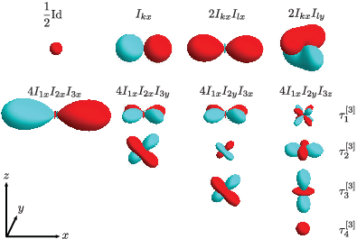
The only droplet for a linear Cartesian product operator on spins consists of two spheres which are colored red and cyan, while the red one corresponds to a positive sign and points into the direction of the axis (see Fig. 2). More generally, the axis of the droplet for a Cartesian operator with is collinear and proportional to the vector . This corresponds to a vector generalizing respectively a (magnetic) field vector for Hamiltonians and the Bloch vector for density matrices, which represents the magnetization in nuclear magnetic resonance (NMR) [3] or polarization in quantum optics [4, 13].
Bilinear Cartesian operators on spins and with such as an anti-phase coherence operator [3] with and induce a droplet with a particular shape (see in Fig. 2) which is not common for atomic or molecular orbitals. This droplet consists of two bean-shaped lobes with colors red and cyan whose major axes are orthogonal to each other. The major axis of the red lobe is oriented in the direction , while the axis from the cyan lobe to the red one points in the direction given by the right-hand rule. The droplet transforms naturally under rotations, e.g., when both spins are simultaneously rotated by around the -axis, the anti-phase operator is mapped to corresponding to a droplet of the same shape but with inverted colors. More general shapes appear for the bilinear operators in the form of elongated shapes as well as antisymmetrically elongated shapes oriented along the -direction for the trilinear operators (see Fig. 2).
IV.2 Multiple quantum coherences
Operators of defined coherence order play an important role in NMR spectroscopy [3]. They are invariant under global -rotations up to a phase factor:
This property is nicely captured in the DROPS representation as detailed in Appendix C.1, where characteristic multiple-quantum terms for linear, bilinear and trilinear operators are displayed in the LISA basis.

IV.3 Hamiltonians
Hamiltonians can also be conveniently visualized using the DROPS representation. The cases of linear and bilinear terms of the Hamiltonian mirror the properties of Cartesian product operators as discussed above. We analyze the shape of the droplets for bilinear coupling Hamiltonians
representing characteristic spin-spin interactions (see, e.g., Fig. 3): The cases and correspond to the Ising- (or Heisenberg-Ising) model [75, 76], which is also known as weak [3] or longitudinal coupling [77] and is represented by a longitudinally elongated droplet. The Heisenberg- model with and is also denoted as strong or isotropic coupling [3] and results in an isotropic droplet of spherical shape. For and , we obtain the Heisenberg- model which is also know as the planar coupling [78, 77] and is represented as a planar disc-shaped droplet in the - plane. The case and corresponds to a dipolar coupling . More general coupling terms can also be visualized. Examples as anisotropic Heisenberg or effective trilinear coupling terms could be used in visualizations of multi-spin systems such as the well-known Kitaev honeycomb lattice [79]. Hence, even for very large spin systems the LISA basis (presented here explicitly for three spins) can be used to visualize Hamiltonians with at most trilinear terms.

IV.4 Time evolution
We provide an example visualizing density operators, Hamiltonians, and unitary transformations for a non-trivial pulse sequence in NMR spectroscopy (see Fig. 4); full details are given in Appendix C.2. The pulse sequence consists of two pulses separated by a delay, which is designed to excite triple-quantum coherence starting from the thermal density operator in the high-temperature limit [3]. This highlights crucial information for the system and provides a better understanding of the corresponding time evolution. Note that the unitary transformation is not hermitian and therefore requires in general more colors.

IV.5 Pure quantum states
In the field of quantum information [5], (in addition to mixed states) pure states and their entanglement measures are of particular interest. Density matrices for four examples of pure states are visualized in Fig. 5: a product state and a maximally-entangled Bell state for two spins as well as the W state and the Greenberger-Horne-Zeilinger state for three spins (further cases are given in Appendix C.3). The reduced density matrix of a two-spin system is obtained by tracing over the second spin which translates into deleting in the LISA basis expansion all linear terms corresponding to the second spin and all bilinear terms. Let denote the maximal radius of the droplet for the first spin, i.e. the maximal absolute value of the spherical function (cf. Eq. (4)) for the corresponding linear terms. Thus, the length of the Bloch vector corresponding to is given by for -spin systems.
As an example for an entanglement measure for two spins, consider the concurrence [80] which can be expressed as a function of (see also [81], [82, p. 168], or [83, p. 50]). Hence, it can also be obtained from the maximal radius as . The value of the concurrence for the pure state and of Fig. 5 is zero and one, respectively.
For the three-spin examples in Fig. 5, interesting information about their bipartite entanglement measured by the concurrence [84, 85, 86] can be directly deduced form the size of the droplets corresponding to linear terms. As the linear terms in the LISA basis expansion are very small for the W state , each spin is strongly entangled with the rest of the system [85]. For , the linear terms in the LISA basis expansion are even zero implying that each spin is maximally entangled with the rest of the system [84, 85].
The preceding examples highlight that a DROPS representation using the LISA basis implicitly includes all reduced density matrices. A reduced density matrix is obtained by deleting all droplets (or terms in the LISA basis) which correspond to spins which have to be traced out. This should be particularly instrumental in visualizing quantum states while emphasizing their symmetries and entanglement properties.
V Generalized Wigner representation
In this section we describe how the DROPS representation can be interpreted as a generalized Wigner function. Recall that the Wigner quasi-probability distribution (or Wigner function for short) provides an equivalent phase-space formulation for the standard Hilbert-space framework of quantum mechanics and mimics the phase-space probability distribution in classical physics [87, 88, 89, 90, 91, 92, 93, 94, 4, 95, 96]. It is formally not a probability distribution as negative values may appear. These negative values in Wigner functions might be interpreted as signatures of quantum effects (cf. [97]). However, the scope of this interpretation is still widely discussed in the literature [98, 99, 100, 101, 102, 103, 104, 105, 106, 107, 108]. Although Wigner functions were originally developed for infinite-dimensional quantum systems with continuous degrees of freedom, they can be extended to finite-dimensional quantum systems following the work of Stratonovich [109], see, e.g., [110, 111, 112]. For the finite-dimensional case, a different perspective is provided by a comprehensive theory of square-integrable functions on compact Lie groups (e.g., functions on the sphere for ) introduced in the seminal work of Peter and Weyl [113] (see [35]). The case of non-compact Lie groups is still an area of active research [114, 115]. However, a relatively simple example of a non-compact Lie group is the symplectic group which is widely studied in quantum optics [116] in the context of infinite-dimensional systems.
Returning to Wigner functions of finite-dimensional systems, the case of one spin (and a “collection” of spins) was detailed in [117, 118, 15] where each tensor operator is mapped to a unique (square-integrable) function on a sphere along the lines of Eq. (2). In these spherical plots, qualitative signatures of quantum effects such as “oscillating fringes” and “interference patterns” have been analyzed in [15, 119, 120, 19, 121]. But similarly as for the above discussed infinite-dimensional Wigner functions the significance of these qualitative signatures is still debated in the literature. For example, Refs. [122, 123, 97] state that quasi-probability distributions corresponding to states and measurements are necessary for reliably detecting quantum effects from negative values. A different strategy for visualizing entanglement properties of quantum states could be based on the localized information in the LISA basis. A first example in this direction is given in Sec. IV.5 where pure quantum states are analyzed with the help of reduced density matrices.
The approach of Stratonovich [109] defines a “spherical phase space” [97]. But the general case of Wigner functions for coupled spin systems has not been solved so far [17, 19]. Therefore, it is important to point out that the approach introduced in this work (c.f. Eq. (4)) provides in fact a solution to this open problem. Rather than mapping each operator to a single function on a sphere (see Eq. (2)), it is mapped to a set of functions on multiple spheres. This set satisfies conditions generalizing the ones of Stratonovich [109, 111, 112] and hence can be interpreted as a generalized Wigner function:
Proposition 1
We assume
that the DROPS representation of Eq. (4) observes the Condon-Shortley phase convention
and that the functions
are correctly normalized. The following conditions are fulfilled:
(a) Linearity:
is linear for each .
(b) Reality: holds for each .
(c) Norm: .
(d) Covariance: holds for
each and all non-selective rotations ,
(e) Trace: .
The (inversely) rotated point on the sphere has the coordinates . The corresponding action describes a non-selective spin conjugation where the unitary matrix is a non-selective rotation operator (acting on complex column vectors, in particular on quantum-mechanical Hilbert-space vectors). The straightforward proof of Prop. 1 is given in Appendix D. Based on these criteria, it is possible to describe the state of spin systems using droplets, i.e. sets of linear combinations of spherical harmonics. In particular, for a given set of droplets, the expectation value of an operator can be calculated based on (e), where is replaced by the density operator : . The relations of Prop. 1 are obtained from the Stratonovich conditions in a straightforward fashion by simply applying them to each droplet individually (for (a), (b), and (d)) or by summing over all the droplets (for (c) and (e)). Note that in contrast to the original Stratonovich conditions, in (c) the function appears. This is a direct consequence of (e) if is replaced by the identity operator. It ensures that unwanted contributions from functions with traceless are eliminated. Consider for example the traceless basis operator for two spins which is mapped to on one droplet. Without the presence of , (c) would result in , which is a contradiction. For the special case of a single spin, the only droplet with rank corresponds to the identity operator and the generalized criterion (c) given above can be reduced to the original form of Stratonovich. As the integrals vanish for anyway, the only terms contributing to (c) come from the cases with corresponding to the spherical harmonic . In the case of the LISA basis, the identity operator is mapped to a unique droplet as the basis operators are also characterized by particle number. Then, the sum in (c) reduces to a single term with the integral corresponding to this particular droplet while ignoring all the other ones.
VI Arbitrary number of spins
We demonstrate now to what extent the construction of the LISA basis (as outlined in Sec. III and detailed in Appendix B) is applicable to an arbitrary number of spins. It is explained that the available quantum numbers (or the corresponding symmetries) are sufficient for labeling a tensor operator basis of the full quantum system or that the quantum numbers can be easily extended with ad-hoc labels. In particular, no ad-hoc labels are necessary for up to five spins. Our analysis also identifies the inherent symmetry structure of the quantum system and provides specifics on the number of droplets for the LISA basis. Moreover, lower and upper bounds for the number of droplets are given for general DROPS representations.
To this end, we resume discussing the choice of labels which provides a partition of the irreducible tensor operators into subsets never containing tensor operators of rank more than once (see (3)). This partition induces also a decomposition into different droplets for the DROPS representation. Recall that the number of droplets for three spins is bounded by . Bounds for up to twelve spins are given in Table 2.
In the particular case of the LISA tensor operator basis, the irreducible tensor operators of rank are divided according to the number of spins involved, the set of involved spins, and the symmetry type under permutations of the set . All possible combinations of , , , and for up to three spins are shown in Table 1, where the notation was simplified by suppressing some trivial symmetry types. Below, we will explain the labels of Table 1 for an arbitrary number of spins and provide a general method for computing all possible combinations of rank and symmetry type reflecting both the symmetries of the unitary group and the symmetric group . This also determines the number of droplets for the LISA basis as shown in Table 2.
We infer from Table 2 that the number of droplets is significantly smaller than the dimension of the operator space for spins. Moreover, the LISA basis uses more droplets than strictly necessary. But meaningful labels are essential as even the minimum number of droplets grows very fast. Therefore, each droplet of the LISA basis has a unique permutation symmetry type except for bilinear operators, where the two occurring symmetry types (e.g., and ) are combined into one droplet which is possible as no -value appears more than once. Based on the values in Table 2, we consider the LISA basis as an efficient and informative visualization for a moderate number of spins. In the following, we first present a method for computing the minimum and maximal number of droplets for a DROPS representation. Secondly, we describe the explicit form of the labels for the LISA basis and thereby determine the corresponding number of droplets.
| number of droplets | |||||
|---|---|---|---|---|---|
| minimum | multipole | LISA | maximum | ||
| 1 | 1 | 1 | 2 | 2 | 0.250 |
| 2 | 3 | 4 | 4 | 6 | 0.188 |
| 3 | 9 | 9 | 11 | 20 | 0.141 |
| 4 | 28 | 36 | 36 | 70 | 0.109 |
| 5 | 90 | 100 | 122 | 252 | 0.088 |
| 6 | 297 | 400 | 423 | 924 | 0.073 |
| 7 | 1001 | 1225 | 1486 | 3432 | 0.061 |
| 8 | 3640 | 4900 | 5246 | 12870 | 0.056 |
| 9 | 13260 | 15876 | 18689 | 48620 | 0.051 |
| 10 | 48450 | 63504 | 67356 | 184756 | 0.046 |
| 11 | 177650 | 213444 | 244917 | 705432 | 0.042 |
| 12 | 653752 | 853776 | 896899 | 2704156 | 0.039 |
VI.1 The minimum and maximal number of droplets
Recall that the set of infinitesimal rotation operators (or equivalently the Lie algebra ) acts on the irreducible tensor operators and of a single spin via (1). This means that the unitary group (and its Lie algebra ) acts for a single spin non-trivially on a three-dimensional (complex) space via its three-dimensional irreducible representation . Here, an irreducible representation of denotes in the language of representation theory [124, 35, 47] an action of on the abstract space (for which the irreducible tensor operator provides an explicit model) and maps an element to a matrix .
|
|
|
For multiple spins, a simultaneous action of on (e.g.) all -linear operators of an -spin system arises and the (inner) tensor product representation of naturally acts on the -fold tensor product of a three-dimensional (complex) space. The tensor product representation is known as the th tensor power of and decomposes into a sum of representations with multiplicities by means of the well-known technique of Eq. (6) (for general methods, cf. pp. 424–429 of [124] or pp. 135–142 of [125]). The explicit values for in Table 3 have been computed using the computer algebra system magma [126]. The corresponding multiplicities for the full -spin system are obtained by summing the multiplicities for -linear operators with which have to be multiplied with the number of possible sets of spins. For example consider the number for spins with rank . Here, for the set we find and for each of the sets , , and we have which can be inferred from the corresponding case of two spins. None of the subsets yields an operator with rank and the corresponding -values are zero. Thus, . For a given , the minimum and maximal number of droplets in Table 2 are now given by the maximum of the multiplicities for all ranks and the sum , respectively.
VI.2 All combinations of symmetry types
We determine all possible combinations of rank and permutation symmetry type by refining our symmetry analysis of -linear operators. Before, we identified the symmetries of -linear operators for rank which are modeled by a -fold tensor product and acted on by the unitary group . We extend this action on to an action of the direct product , where the symmetric group acts by permuting spins from a set with .
|
|
The corresponding symmetry analysis for the number of spins is summarized in Table 4, where we consider -linear operators with in a -spin system. Table 4 states all possible combinations of rank and partition from which the corresponding permutation symmetry types can be easily determined. A partition of length and degree consists of positive integers with and can be identified with a Young diagram (i.e. a Young tableaux without entries) which is a left-aligned arrangement of boxes into rows where the th row contains boxes (cf. pp. 44–45 of [124]). The number of different symmetry types for each partition is given in the third column () of Table 4. The results for and some partial results for can also be found in Table 12 of [127] (cf. Table 2 on p. 294 of [67]).
Combinations of and which appear more than once are highlighted in Table 4. The case of and for has been known at least since [128] (see also [127, 74]). If no combination of and appears more than once (as for ), the LISA basis is uniquely defined without any additional labels. This ensures that the visualization technique described in this work is directly applicable for up to five spins. Additional labels are required in the general case, but ad-hoc labels as in [128] are usually sufficient. The resulting permutation symmetry types for a partition are given by the standard Young tableaux of shape [44, 45, 46, 47], i.e. Young diagrams of shape which are filled with the numbers from the set of the involved spins. The employed method for the computation of Table 4 is a combination of the Schur-Weyl duality [129] and a technique known as plethysm [130, 131, 132, 43]. The results in Table 4 were obtained using the computer algebra system magma [126] and details are given in Appendix E.
We explain now how to read Table 4 and how to recover some of the labels for the three-spin case of Table 1. In particular, we consider the subsystem of trilinear operators (i.e. and ). Referring to the case of in Table 4, we obtain the combinations of and , and , and , and , as well as and . Note that induces the permutation symmetry (using the notation of Eq. (5)). Similarly, one obtains and for as well as for . Consequently, all the relevant labels in Table 1 can be recovered.
VII Discussion
Before concluding, we discuss alternative DROPS visualizations which complement the LISA representation. A suitable choice can reflect the considered system and application. One possibility arises form partitioning the tensor operators from the Clebsch-Gordan decomposition of Eq. (6) into droplets without symmetrizing with respect to spin permutations as in the LISA basis. As before, one has to ensure that no rank appears more than once in any droplet. Many different partitions are possible, and applying the Clebsch-Gordan decomposition recursively could provide a natural partition.
Indistinguishable spins utilize only a proper subspace of all tensor operators. The corresponding symmetry-adapted tensor basis can be obtained by symmetrizing tensor operators with respect to the relevant spin permutations. This usually reduces the number of droplets. In particular, one can discard all droplets with incompatible symmetry types. For example, the Hamiltonian and the density operator in a three-spin system of type [133, 3] are both invariant with respect to permutations of the first two spins. Consequently, the LISA basis can be restricted to a -dimensional space consisting of the twelve irreducible tensor operators , , , , , , , , , , , and . This allows us to reduce the number of droplets from eleven to seven. For a three-spin system which is totally symmetric with respect to spin permutations, the LISA basis can be limited to a -dimensional space spanned by the tensor components of the six irreducible tensor operators , , , , , and . Thus, one obtains four droplets.

One further variant of the DROPS visualization is based on multipole tensor operators [134, 63, 135, 136, 137, 138] which reflect the state-space structure of angular momentum states with suitable-chosen auxiliary labels. The multipole tensor operators are defined by means of transforming one set of states of defined rank into another one according to the Clebsch-Gordan decomposition , where . The multipole tensor operators differ from the tensor operators in the LISA basis in not having a defined particle number (i.e. linearity) and inducing a different grouping into droplets (see Appendix F). The corresponding number of droplets is given in the column named multipole of Table 2 and can be computed as the square of the number of irreducible tensor operators (with multiplicity). The multipole-based DROPS representation introduced here can be viewed as a generalization of the special Wigner representation introduced in [18] for a spin particle coupled to a second particle of arbitrary spin number. Figure 6 illustrates the DROPS representation based on multipole operators using the same pure-state examples which are shown in Fig. 5 for the LISA basis. In contrast to Fig. 5, in Fig. 6 all examples have only one single non-empty droplet.
VIII Conclusion
We introduced a general approach for representing arbitrary operators by a finite set of functions. Their properties make this representation particularly appealing and useful for the visualization of important quantum mechanical concepts and properties, which are conventionally represented by abstract operators or plain matrices. There are many possible bases on which such a mapping between operators and sets of functions can be based. Here we focused on the LISA basis which transforms naturally under non-selective spin rotations as well as spin permutations and which is particularly suitable for distinguishable spins. However, depending on the application, other bases can be more appropriate. It is noteworthy that the DROPS visualization can be seen as a generalization of the Bloch vector representation of simple two-level quantum systems, such as uncoupled spin 1/2 particles. On the other hand, the DROPS method can also be interpreted as a natural (albeit not obvious) generalization of Wigner functions that have been studied extensively for “collections” of spins. The physical interpretation of the DROPS representation in terms of a quasi-probability distribution for experimental observables and the related question of non-classical signatures are interesting open problems. These are however beyond the scope of the present work, which focusses on the theoretical construction and the symmetry properties of the DROPS representation.
Although we considered here the relatively simple but non-trivial example of three coupled spins 1/2, our method can also be applied to more than three spins and is also not limited to spins 1/2. It is important to emphasize that general coupled spin systems constitute complex high-dimensional quantum systems whose description cannot be expected to be both complete and simple. We outlined in the beginning of Sec. II the essential properties which our visualization should satisfy. These properties can be summarized as (A) the bijectivity of the mapping and (B) the immediate visibility of crucial features (such as symmetries under non-selective rotations). Under these assumptions, the analysis of Sec. VI (see Table 2) rules out a complete representation of operators with only a single droplet for spin systems with more than one spin. In contrast to that, the visualization technique of Ref. [19] (see also [117, 118, 15]) uses only a single droplet (even for more than one spin). Therefore, in general, it cannot respect all symmetries of operators under non-selective rotation and be complete at the same time. The approach of [19] emphasizes the structure of pure quantum states and chooses quantum numbers from the eigenvalues of the operators and , where with . But this captures only a subset of the symmetries of pure quantum states under non-selective rotations. All these symmetries are revealed by directly applying the Clebsch-Gordan decomposition of the tensor product structure. Hence, the approach of [19] could be modified into a DROPS visualization using the multipole tensor operators (see Sec. VII and Appendix F), which also emphasizes the structure of pure quantum states. In summary, we believe that the analysis of coupled spin systems should be primarily guided by finding their inherent symmetries. This provides a solid foundation for studying nontrivial properties of general spin systems.
We illustrated applications which benefit from the DROPS approach, such as the visualization of mixed quantum states of spin systems. It can also used to represent the density matrix of pure quantum states with or without entanglement. Section IV.5 contains a first step in understanding how entanglement properties of quantum states can be visualized in the LISA basis. Furthermore, the DROPS representation can be applied to arbitrary operators, including Hamilton operators and time evolution operators. This approach is also well suited to show the time evolution of quantum mechanical operators as animations, rather than static figures. The DROPS visualization lends itself to building intuition about the dynamics of coupled spins and is expected to become a valuable tool both in education and research. Potential applications range from theoretical and experimental quantum information theory, where quantum bits (corresponding to spins ) can be realized by trapped ions, quantum dots, superconducting circuits, and spin systems, to electron and nuclear magnetic resonance applications in physics, chemistry, biology, and medicine. A Mathematica package [139] and a mobile application software [140] are made available so that readers may apply the DROPS mapping to new areas and interactively explore the DROPS visualization of coupled spin dynamics in real time.
Acknowledgements.
The authors acknowledge support from the Deutsche Forschungsgemeinschaft (DFG) via the grant GL 203/7-1 and the SFB 631 as well as from the EU programmes QUAINT and SIQS. A.G. was supported by NSERC (Canada). R.Z. was also funded by the DFG through the grant SCHU 1374/2-1.Appendix A Motivation for the choice of signs in the LISA basis
The phase of the irreducible tensor operators for the LISA basis is fixed by the Condon-Shortley convention up to a sign. The specific choice of signs made in the LISA basis will be presented in Appendix B.3, during the construction of the LISA basis via projectors (see, e.g., Table ). Here, we present desirable properties which motivate this specific choice of signs:
The droplet of the identity operator has a positive value (i.e. it is red in Fig. 2). The droplets of the linear Cartesian operators with for each spin are consistent with its Bloch vector representation, i.e., the positive lobe in the LISA visualization of is pointing in the -direction (see Fig. 2).
Characteristic coupling Hamiltonians, such as longitudinal and planar couplings have elongated and disc-shaped droplets (see last column of Fig. 7). For spins and , different shapes appear if and have different relative signs (Fig. 7). If the sign of is negative, the positive lobe of the droplet representing with (refer to case c) in Fig. 7) is displaced in the -direction with respect to the center of the droplet, where is given by the right hand rule. The droplet for the fully symmetric Cartesian tensor has an elongated shape and its positive lobe points in the direction (see Fig. 2).

Appendix B Construction of the LISA basis via projectors
We provide here the details for the iterative construction of the LISA basis which is directly applicable to general spin systems with spins. We determine the basis elements by applying explicit projection operators. The presentation aims at providing all necessary details for replicating our approach. To this end, we specify also all applied conventions which regrettably vary significantly in the literature.
B.1 The symmetric group and the standard Young tableaux
We start by recalling some basic notation, see, e.g., [44, 45, 46, 47]. The permutations of a set of cardinality are known as the symmetric group . They form a finite group whose group multiplication is defined by the composition for and . An element maps to such that for . Permutations can be compactly specified as products of disjoint cycles. A cycle of length (where and for ) represents a permutation where for and . Two cycles and are disjoint if for all and . A transposition with is a cycle of length two which permutes and . Note that the symmetric group acts naturally on the set of Cartesian product operators (for notation refer to Sec. IV.1) by permuting particles (and their labels), e.g., for . This is equivalent to setting for spins with .
Recall that a standard Young tableau of size is a left-aligned arrangement of boxes where the number of boxes does not increase from one row to following ones and where each box contains a different number from the set such that the numbers are ordered strictly increasing from left to right and top to bottom. For every standard Young tableau , one introduces a partition (i.e. its shape) of length where the positive integers with are equal to the number of boxes in row of and agrees with the number of rows of . The number of columns of is equal to . Also, the filling pattern of consists of the entries of which are strung together from left to right in each row and from top to bottom for all rows. It is convenient to introduce a total order on the set of standard Young tableaux of size where if either or if and . Here, we imply that if there exists an index such that for and while setting for and for . This total order for standard Young tableaux is reflected by the subscript in the notation introduced in Eq. (5), e.g.,
| (7) |
B.2 Young symmetrizers and projectors
We detail now the construction for Young symmetrizers and the corresponding projectors with symmetry type [44, 45, 141, 142, 47, 129, 143, 144, 63, 64]. These objects are elements of the group algebra of which consists of all (formal) real linear combinations of permutations . This means that every element can be decomposed as with coefficients . Given two elements , the sum in is naturally defined as and the product is given by .
Given a standard Young tableau , let [resp. ] denote the set of all entries in the th row [resp. th column] of . Let denote the permutations of a set and let us introduce the permutations of the elements in the th row of the standard Young tableau where . In the example of , one obtains and as well as and where denotes the identity permutation. The set of row-wise permutations is now defined as . Note that the order in the product is irrelevant as the different permutations act on non-overlapping subsets of . For , we have . Similarly, we obtain the set of column-wise permutations where . One introduces and where denotes the minimal number of transpositions necessary to write as product thereof. Finally, we can write the Young symmetrizer for as the product where the normalization factor is equal to the number of standard Young tableaux of shape divided by which ensures that . For instance, the Young symmetrizers for the standard Young tableaux of Eq. (7) are
| (8a) | ||||
| (8b) | ||||
| (8c) | ||||
| (8d) | ||||
where denotes the identity in and one directly verifies that . The Young symmetrizer can be computed (e.g.) for Eq. (8c) by multiplying , , and where .
We determine now projectors (i.e. ) which can be interpreted as orthogonalized versions of the operators in Eq. (8). These projectors model the symmetries for a standard Young tableau and will be used to identify tensor operators which are left invariant under their action, i.e. for all . Our approach for determining the projectors is similar to the one detailed on pp. 114–124 of [141] and the formulas can be inferred from the matrices of Young’s seminormal or orthogonal representation [44, 45, 142, 143]. But we stress that the employed formulas differ widely in the literature due to varying conventions. Note that we obtain a basis of projection operators which differs from the so-called seminormal basis (cf. pp. 109–114 of [142]).
Let us consider the ordered sequence of all standard Young tableaux of fixed shape . In particular, one has for , and for , as well as for (cf. Eq. (7)). One defines the projection operators recursively using the operators : For , one has . It immediately follows that
| (9) |
For , there exists such that differs from only by the position of two boxes and with consecutive labels and . Let denote the signed axial distance from the box to in , i.e., the number of steps from to while counting steps down or to the left positively and steps up or to the right negatively. After these preparations, we set
| (10) |
where the scalar factor is chosen such that . For , one obtains , , , , and Eq. (10) implies that
| (11) |
B.3 Details of the iterative construction
The iterative construction of the LISA basis is now described and exemplified for the example of spins. In the Sec. III.2, this construction was divided into three steps: (I) We start by building and symmetrizing -linear tensor operators of a -spin system for each which consists in applying the Clebsch-Gordan decomposition and the just-introduced projection operators. (II) Next, the tensor operators will be phase and sign corrected. (III) Lastly, the tensor operators are embedded into the full -spin system for each -element subset of .
In step (I), we begin by specifying the form of the -linear tensor operators for a -spin system in the particular simple cases of . The symmetries with respect to particle permutations are trivial in both of these cases. The corresponding symmetry types are given by the standard Young tableaux and where the first one is empty and the second one consists of a single box. For , we only have the tensor operator whose only tensor component is given by . There is one single linear tensor operator for whose components are , , and .
For , the tensor operators for spins are combined with the tensor operator for one spin in order to iteratively build up the tensor operators with for spins using the Clebsch-Gordan decomposition . The corresponding tensor components with are determined by the Clebsch-Gordan coefficients [21, 26, 27]. The three bilinear tensor operators , , and for are obtained via and their components are given by (see, e.g., p. 419 in [62])
The projectors for are
ItisobviousthatP^[2]_1 T^[2]_0,0 = T^[2]_0,0P^[2]_1 T^[2]_2,m = T^[2]_2,mm ∈{-2,…,2}P^[2]_2 T^[2]_1,m = T^[2]_1,mm ∈{-1,0,1}T^[2]_0T^[2]_2τ_1^[2]T^[2]_1τ_2^[2]g=3T_0,0”P^[3]_4T_0,0” = P^[3]_4 T_0,0”P^[3]_1 T_0,0” = P^[3]_2 T_0,0” = P^[3]_3 T_0,0”=0T_0,0”T_0,0”m∈{-3,…,3}T_j,m(τ)Tr[T^_j,m(τ) T_j,m^†(τ)]=1Tr(A) =∑_p A_ppAT_j(τ)T_j(τ)ggnn≥gn=3T_0,0(τ_1^[0])=T_0,0= ( 1 0 0 1 )/ 2 g=01_qq×qT_1(τ_1^[1])g=1n=3m ∈{-1,0,1}g≥1(1k)T^{1}_1,m(τ_1^[1])kT_j,m(τ_p^[2])m∈{-j,…,j}n≥2m∈{-j,…,j}
B.4 From the LISA basis to Cartesian product operators
Before we close this section, our computations are summarized by providing explicit basis transformations from Cartesian product operators (for definitions refer to Sec. IV.1) to the LISA basis and vice versa. The basis transformations for the linear tensor components of an -spin system are
Similarly, the transformations in the bilinear case are
The decomposition of trilinear LISA tensor components in terms of the trilinear Cartesian-product basis is detailed in Table , while the other direction can be found in Table 7; observe the shorthand .
Appendix C Visualization of typical operators in the LISA basis
C.1 Visualizations of multiple quantum coherences
Different examples of multiple-quantum coherences are given in Fig. 11. Operators with defined and unique coherence order are visualized in the third and fourth column of Fig. 11 for and , respectively. The operators displayed in the first and second column of Fig. 11 correspond to mixtures of multiple quantum orders .
As discussed in Sec. IV.2, an operator has a well-defined coherence order if a rotation around the z axis by an arbitrary angle reproduces the operator up to an additional phase factor :
Similarly, a droplet representing a function (c.f. Eq. (4)) corresponds to an operator term with well-defined coherence order , if a rotation around the -axis by an arbitrary angle reproduces the droplet (and the function ) up to an additional phase factor . Hence, a droplet with coherence order as well as the corresponding function are transformed by a -rotation with angle to with . In order to illustrate this point, consider how the operator in Fig. 11 with changes under a -rotation with angle . A -rotation of the corresponding droplet only changes its color (representing the phase of the function ) but not its shape. For example, for the azimuthal angle , the droplet is red (corresponding to a phase ). After the rotation by , the droplet has turned dark blue at the azimuthal angle (corresponding to a phase ), which is exactly what is expected from the general formula given above: for and .
Based on these properties, the droplets of an operator with unique coherence order can be easily recognized using the following criteria: (1) Disregarding the color, the shape of the droplet is rotationally invariant under rotations around the -axis, i.e. the shape is not changed by a -rotation (c.f. third and fourth column in Fig. 11). (2) The coherence order of a droplet can be identified based on its color: (2a) A droplet of coherence order does not change its color if it is rotated by an arbitrary angle around the -axis, as illustrated by the operators , , , and in Fig. 11. (2b) A droplet of unique coherence order (where is a non-zero integer with either positive or negative sign) is rainbow-colored. For positive coherence order (), the colors change from red to yellow to green to blue when moving counter-clockwise around the -axis. For negative coherence order, the colors change in the opposite direction. (2c) For a non-zero unique coherence order , the absolute value of the coherence order of a droplet is reflected by the number of rainbows encountered when moving once around the -axis. (2d) A droplet of unique coherence order is invariant under a rotation by integer multiples of around the -axis. This is illustrated for characteristic operators with unique coherence orders in the third column and fourth column of Fig. 11. (2e) Even if operators do not contain a unique coherence order , but a mixture of coherence orders with , it is still true that the corresponding droplets do not change their appearance if they (or the corresponding operators) are rotated by integer multiples of around the -axis. This is illustrated by the examples in the first and second column of Fig. 11. All tensor operators have the unique coherence order . Moreover, the bean-shaped droplet of the Cartesian product operator (c.f. Fig. 8) is an example of an operator that is composed of terms with different coherence orders , 0, and . The operator is a superposition of the double-quantum operator with rank and quantum orders and the zero-quantum operator with rank and quantum order .

C.2 Extended NMR example
The example shown in Fig. 12 represents a common experiment in NMR spectroscopy which is designed to create triple-quantum coherences from the polarization of three coupled spins [3]. The system consists of three spins in the weak-coupling limit (i.e. longitudinal or Ising-type coupling; see Fig. 3) with identical coupling constants . The building blocks of the experiment are visualized in Fig. 12 in the LISA basis. A triple-quantum coherence consists of combinations of tensor operators of rank and order . At the initial time , the system is in thermal equilibrium, which corresponds in the high-temperature limit to the density matrix
(where for simplicity only the traceless part of the density operator is considered here).
A first pulse (with phase ) is applied to the system with an amplitude of for a time and flips the three magnetization vectors into the transverse plane. The corresponding linear control Hamiltonian is
and the density operator of the system at time is
The next step consists of letting the bilinear coupling Hamiltonian act on the system in order to create trilinear terms in the density operator. The coupling Hamiltonian is applied for a time and has the form
At time , the systems is in the state
Finally, a second pulse (with phase ) is applied in order to create terms of order . The corresponding linear control Hamiltonian
is applied for a time At time , the density operator of the system is (where )
At this point, the desired triple-quantum coherence term has been created. Note that the shape of the droplet corresponding to the term of in Fig. 12 also exhibits the partial content of the triple-quantum coherence (see Fig. 11). The remaining undesired terms of the density operator can be removed by applying a triple quantum filter [3] to (not shown for simplicity). The density operators are depicted in the middle row of Fig. 12.
The Hamiltonians (which are re-scaled for better visibility) are shown in the second row and the effective Hamiltonian [3]
of the experiment is given at the top. In the fourth row, the DROPS representations of the propagators ( denotes the -dimensional identity matrix)
are shown. The overall effective propagator
of the pulse sequence is given at the bottom of Fig. 12.

C.3 Pure quantum states
The examples of Fig. 9 display density matrices for entangled pure states of two spins and three spins in the DROPS representation corresponding to the LISA basis. The four Bell states and correspond to maximally entangled states of a two-spin system. For comparison, a separable state () and a partially entangled state are depicted in the third row of Fig. 9. The last row of Fig. 9 shows the W state and the Greenberger-Horne-Zeilinger state , which are both entangled quantum states of three spins.
Appendix D Wigner representation: Proof of Proposition 1
Property (a) is a direct consequence of the definition of the DROPS mapping. Proving property (b), we deduce directly from Eq. (4b) that
Consequently, (b) follows from the Condon-Shortley phase convention and a similar relation for spherical harmonics. Property (c) is a special case of (e), which we prove below. Property (d) uses the fact that irreducible tensor operators and spherical harmonics are an explicit form of irreducible representations for . These properties are preserved by the DROPS mapping, i.e., the components with corresponding to the same tensor define an invariant subspace under rotations. Furthermore, all of these components are part of the same droplet. The proof of property (e) requires a more detailed analysis. We expand both sides of (e) in order to show that they are equal. To simplify the notation, the dependence of the spherical harmonics on the variables and is suppressed.
The left-hand side of the equality is expanded as , which is equal to
Applying the orthonormality of the spherical harmonics as well as the property , we obtain the expression . Applying , this can be further simplified to .
On the right-hand side, we have
by the linearity of the trace, which can be further transformed to relying on the orthogonality of the operator spaces for different droplets. We use the decompositions of the and and obtain the formula
Using the normalization and , it simplifies to . This shows that the left-hand side is identical to the right-hand side.
![[Uncaptioned image]](1409.5417v2/tensor_filter_multipole_graph.png)
Appendix E Details for the computation of Table 4
Here, we detail the computations summarized in Table 4. These are determined in two steps. First, the symmetries of the direct product acting on (notably for ) are identified, where denotes the general linear group of complex -matrices with non-zero determinant. The irreducible representations of are labeled by partitions with at most parts (i.e. ), cf. pp. 231–237 of [124], and irreducible representations of the symmetric group are indexed with partitions of degree , cf. pp. 44–46 of [124]. Using these notations, the Schur-Weyl duality (see p. 389 of [129]) describes how the action of decomposes -tensors into a multiplicity-free sum (i.e. each occurs only once)
| (13) |
where denotes the set of partitions with degree and with at most parts (i.e. ).

|
|
|
| ||||||||||||||||||||||||||||||||||||||||||||||||||||||||||||||||||||||||||||||||||||||||
Second, these results will be traced back to the intended group . Here, since (and its Lie algebra ) acts for a single spin on the three-dimensional space as explained in Sec. VI. We substitute in Eq. (13) by the composition to include the action of on . The decomposition of as a representation of is determined by applying the well-established technique of the plethysm [130], see also [131, 132, 43]. The explicit computations for the plethysms have been performed using the computer algebra system magma [126], but computations could in this particular case also rely on a generating function, see p. 178 of [145]. The combination of both steps leads to the results of Table 4. The resulting symmetry types for a partition are given by the standard Young tableaux of shape [44, 45, 46, 47], i.e. Young diagrams of shape which are filled with the numbers from the set of the involved spins. The number of symmetry types (with fixed shape and set ) is equal to the dimension of the irreducible representation of (refer to the third column () of Table 4).
Appendix F DROPS representation based on multipole tensors
Multipole tensor operators [134, 63, 135, 136, 137, 138] are defined by building on a state-space basis of the quantum system which reflects its angular momentum properties , where are suitable-chosen auxiliary labels distinguishing angular momentum states with identical rank (and order ). Given and , the symbol denotes the ordered set of states with angular momentum and auxiliary label . Moreover, the state space of coupled spins has a basis . Multipole tensor operators can now be defined by transforming the states into according to the Clebsch-Gordan decomposition
| (48) | ||||
where one assumes that and where denotes the Clebsch-Gordan coefficient. The matrix contains only a single nonzero entry corresponding to the state transition . All multipole tensor operators transforming into have integer ranks running from to and are grouped into a single droplet in the associated DROPS representation. The corresponding labels of Eq. (4) have the form (see, e.g., Table 8).
The angular momentum states are constructed by recursively coupling subsystems with an additional particle. For the case of one spin- particle, the angular momentum state basis is given by . For two coupled spin- particles, we use the Clebsch-Gordan decomposition of and build the basis consisting of singlet and triplet states (see, e.g., pp. 430–431 of [29]). No auxiliary labels are necessary as each rank appears only once in . For three coupled spin- particles, one obtains the basis (see Table 8). The auxiliary labels and of the state refer to the parent rank of the element in involved in its generation. This construction may be in general unwieldy, but it is always possible as is a simply reducible group (see, e.g., [146]), i.e., each irreducible representation in the Clebsch-Gordan decomposition of two irreducible representations of appears only once. All compatible combinations of the nine possible transitions with ranks are given in Table 9. The multipole tensor operators differ from the tensor operators in the LISA basis in not having a defined particle number. The explicit decomposition of multipole tensor operators in the LISA basis can be found in Table 10.
Examples for the DROPS representation based on multipole tensor operators are illustrated in Fig. 10 where the density matrices of different pure states are given (cf. Fig. 9), some of which are entangled and most of them have only one single non-empty droplet. Interestingly, both and exhibit a symmetry under -rotations, i.e. they are respectively rotationally invariant or invariant under rotations of , see also Fig. 9.
References
- [1] R. P. Feynman, F. L. Vernon, Jr., and R. W. Hellwarth, J. Appl. Phys. 28, 49 (1957).
- [2] M. A. Bernstein, K. F. King, and X. J. Zhou, Handbook of MRI Pulse Sequences (Elsevier, Burlington-San Diego-London, 2004).
- [3] R. R. Ernst, G. Bodenhausen, and A. Wokaun, Principles of Nuclear Magnetic Resonance in One and Two Dimensions (Clarendon Press, Oxford, 1987).
- [4] W. P. Schleich, Quantum Optics in Phase Space (Wiley-VCH, 2001).
- [5] M. A. Nielsen and I. L. Chuang, Quantum Computation and Quantum Information (Cambridge University Press, Cambridge (UK), 2000).
- [6] O. W. S\myorensen, G. W. Eich, M. H. Levitt, G. Bodenhausen, and R. R. Ernst, Progr. NMR Spectrosc. 16, 163 (1983).
- [7] D. G. Donne and D. G. Gorenstein, Concepts Magn. Reson. 9, 95 (1997).
- [8] R. Freeman, A Handbook of Nuclear Magnetic Resonance, 2nd ed. (Addision Wesely Longman, Harlow, 1997).
- [9] U. Eggenberger and G. Bodenhausen, Angew. Chem. Int. Ed. Engl. 29, 374 (1990).
- [10] G. Racah, Phys. Rev. 62, 438 (1942).
- [11] J. D. Jackson, Classical Electrodynamics, 3rd ed. (John Wiley & Sons, New York, 1999).
- [12] A. Pines, S. Vega, D. J. Ruben, T. W. Shattuck, and D. E. Wemmer, in Magnetic Resonance in Condensed Matter: Recent Developments, Proceedings of the IVth Ampere International Summer School, Pula, Yugoslavia, edited by R. Blinc and G. Lahajnar (University of Ljubljana, 1976) pp. 127–179.
- [13] T. K. Halstead and P. A. Osment, J. Magn. Reson. 60, 382 (1984).
- [14] B. C. Sanctuary and T. K. Halstead, Adv. Opt. NMR Reson. 15, 97 (1991).
- [15] J. P. Dowling, G. S. Agarwal, and W. P. Schleich, Phys. Rev. A 49, 4101 (1994).
- [16] P. S. Jessen, D. L. Haycock, G. Klose, G. A. Smith, I. H. Deutsch, and G. K. Brennen, Quant. Inf. Computation 1, 20 (2001).
- [17] D. J. Philp and P. W. Kuchel, Concepts Magn. Reso. A 25A, 40 (2005).
- [18] S. T. Merkel, P. S. Jessen, and I. H. Deutsch, Phys. Rev. A 78, 023404 (2008).
- [19] D. Harland, M. J. Everitt, K. Nemoto, T. Tilma, and T. P. Spiller, Phys. Rev. A 86, 062117 (2012).
- [20] E. Wigner, Gruppentheorie und ihre Anwendung auf die Quantenmechanik der Atomspektren (Friedrich Vieweg & Sohn, Braunschweig, 1931) english translation in [21].
- [21] E. P. Wigner, Group Theory and its Application to the Quantum Mechanics of Atomic Spectra (Academic Press, London, 1959).
- [22] D. H. Sattinger and O. L. Weaver, Lie Groups and Algebras with Applications to Physics, Geometry, and Mechanics (Springer, New York, 1986).
- [23] M. E. Rose, Elementary theory of angular momentum (Wiley, New York, 1957).
- [24] A. R. Edmonds, Angular momentum in quantum mechanics (Princeton University Press, Princeton, 1957).
- [25] D. D. M. Brink and G. G. R. Satchler, Angular Momentum (Clarendon Press, Oxford, 1993).
- [26] L. C. Biedenharn and J. D. Louck, Angular Momentum in Quantum Physics (Addison-Wesley, Reading, MA, 1981).
- [27] R. N. Zare, Angular Momentum (John Wiley & Sons, New York, 1988).
- [28] W. J. Thompson, Angular Momentum (John Wiley & Sons, New York, 1994).
- [29] E. Merzbacher, Quantum Mechanics, 3rd ed. (John Wiley & Sons, New York, 1998).
- [30] G. W. Mackey (1981) introduction of [32], pp. xxix–lxxxviii.
- [31] G. W. Mackey (1993) in [33], pp. 241–290.
- [32] L. C. Biedenharn and J. D. Louck, The Racah-Wigner Algebra in Quantum Theory (Addison-Wesley, Reading, MA, 1981).
- [33] A. Wightman, ed., The Collected Works of Eugene Paul Wigner, Vol. I (Springer, Berlin, 1993).
- [34] L. Michel, in Group Representations in Mathematics and Physics, Battelle, Recontres, Lecture Notes in Physics, Vol. 6, edited by V. Bargmann (Springer, Berlin, 1970) pp. 36–143.
- [35] M. R. Sepanski, Compact Lie Groups (Springer, New York, 2007).
- [36] E. U. Condon and G. H. Shortley, The Theory of Atomic Spectra (Cambridge University Press, Cambridge, 1935).
- [37] B. L. Silver, Irreducible Tensor Methods (Academic Press, New York, 1976).
- [38] M. Chaichian and R. Hagedorn, Symmetries in Quantum Mechanics: From Angular Momentum to Supersymmetry (Institute of Physics Publ., Bristol, 1998).
- [39] W. Ledermann, Introduction to Group Characters, 2nd ed. (Cambridge University Press, Cambridge, 1987).
- [40] B. R. Judd, W. Miller, Jr., J. Patera, and P. Winternitz, J. Math. Phys. 15, 1787 (1974).
- [41] R. T. Sharp, J. Math. Phys. 16, 2050 (1975).
- [42] F. Iachello and R. D. Levine, Algebraic Theory of Molecules (Oxford University Press, New York, 1995).
- [43] D. J. Rowe and J. L. Wood, Fundamentals of Nuclear Models: Foundational Models (World Scientific Publ., Singapore, 2010).
- [44] H. Boerner, Darstellungen von Gruppen, 2nd ed. (Springer, Berlin, 1967).
- [45] M. Hamermesh, Group Theory (Addison-Wesley, Reading, MA, 1962).
- [46] R. Pauncz, The Symmetric Group in Quantum Chemistry (CRC Press, Boca Raton, 1995).
- [47] B. E. Sagan, The Symmetric Group, 2nd ed. (Springer, New York, 2001).
- [48] H. Weyl, Gruppentheorie und Quantenmechanik, 2nd ed. (Hirzel, Leipzig, 1931) english translation in [49].
- [49] H. Weyl, The Theory of Groups & Quantum Mechanics, 2nd ed. (Dover Publ., New York, 1950).
- [50] H. Weyl, The Classical Groups: Their Invariants and Representations, 2nd ed. (Princeton University Press, Princeton, 1953).
- [51] J. Listerud, Techniques in Solid State NMR, Ph.D. thesis, University of Washington (1987).
- [52] J. Listerud, S. J. Glaser, and G. P. Drobny, Mol. Phys. 78, 629 (1993).
- [53] A. Chakrabarti, Ann. Inst. Henri Poincaré 1, 301 (1964).
- [54] J.-M. Lévy-Leblond and M. Lévy-Nahas, J. Math. Phys. 6, 1372 (1965).
- [55] H. V. McIntosh, J. Math. Phys. 1, 453 (1960).
- [56] F. P. Temme, Physica A 166, 676 (1990).
- [57] F. P. Temme, Z. Phys. B 88, 83 (1992).
- [58] F. P. Temme, J. Math. Chem. 27, 111 (2000).
- [59] F. P. Temme, J. Magn. Reson. 167, 119 (2004).
- [60] B. C. Sanctuary and F. P. Temme, J. Math. Chem. 43, 1119 (2008).
- [61] J. Schwinger, On Angular Momentum, Tech. Rep. NYO-3071 (U.S. Atomic Energy Commission, 1952).
- [62] Beringer, J. et al. (Particle Data Group), Phys. Rev. D 86, 010001 (2012).
- [63] B. C. Sanctuary and F. P. Temme, Mol. Phys. 55, 1049 (1985).
- [64] W. K. Tung, Group Theory in Physics (World Scientific Publishing Company, Incorporated, 1985).
- [65] G. Racah, in Ergebnisse der exakten Naturwissenschaften, 37. Band (Springer, Berlin, 1965) pp. 28–84.
- [66] J. P. Elliott and A. M. Lane, in Encyclopedia of Physics, Volume XXXIX, Structure of Atomic Nuclei (Springer, Berlin, 1957) pp. 241–410.
- [67] I. G. Kaplan, Symmetry of Many-Electron Systems (Academic Press, New York, 1975).
- [68] C. D. H. Chisholm, Group Theoretical Techniques in Quantum Chemistry (Academic Press, London, 1976).
- [69] P. Kramer, G. John, and D. Schenzle, Group Theory and the Interaction of Composite Nucleon Systems (Vieweg, Braunschweig, 1981).
- [70] H. Hassitt, Proc. R. Soc. London, Ser. A 229, 110 (1955).
- [71] I. G. Kaplan, Soviet Phys. JETP 14, 401 (1962a).
- [72] I. G. Kaplan, Soviet Phys. JETP 14, 568 (1962b).
- [73] H. Horie, J. Phys. Soc. Japan 19, 1783 (1964).
- [74] H. A. Jahn and H. van Wieringen, Proc. R. Soc. Lond. A 209, 502 (1951).
- [75] E. Ising, Z. Physik 31, 253 (1925).
- [76] W. J. Caspers, Spin systems (World Scientific, Singapore, 1989).
- [77] S. J. Glaser, J. Magn. Reson. A 104, 283 (1993).
- [78] T. Schulte-Herbrüggen, Z. Mádi, O. W. S\myorensen, and R. R. Ernst, Molec. Phys. 72, 847 (1991).
- [79] A. Kitaev, Ann. Phys. 321, 2 (2005).
- [80] W. K. Wootters, Phys. Rev. Lett. 80, 2245 (1998a).
- [81] T. J. Osborne and F. Verstraete, Phys. Rev. Lett. 96, 220503 (2006).
- [82] S. Haroche and J.-M. Raimond, Exploring the Quantum: Atoms, Cavities, and Photons (Oxford University Press, New York, 2006).
- [83] J. Stolze and D. Suter, Quantum Computing: A Short Course from Theory to Experiment (Wiley-VCH, Weinheim, 2004).
- [84] W. K. Wootters, Phil. Trans. R. Soc. Lond. A 356, 1717 (1998b).
- [85] V. Coffman, J. Kundu, and W. K. Wootters, Phys. Rev. A 61, 052306 (2000).
- [86] W. Dür, G. Vidal, and J. I. Cirac, Phys. Rev. A 62, 062314 (2000).
- [87] H. Weyl, Z. Phys. 46, 1 (1927).
- [88] E. Wigner, Phys. Rev. 40, 749 (1932).
- [89] H. Groenewold, Physica 12, 405 (1946).
- [90] J. Ville, Cables et Transmission 2A, 61 (1948).
- [91] J. E. Moyal, Proc. Camb. Phil. Soc. 45, 99 (1949).
- [92] L. Cohen, Time-Frequency Analysis (Prentice-Hall, Englewood Cliffs, NJ, 1995).
- [93] U. Leonhardt, Measuring the Quantum State of Light (Cambridge University Press, Cambridge, 1997).
- [94] D. Leibfried, T. Pfau, and C. Monroe, Physics Today 51, 22 (1998).
- [95] R. L. Allen and D. W. Mills, Signal Analysis (IEEE Press, Piscataway, NJ, 2004).
- [96] T. L. Curtright, D. B. Fairlie, and C. K. Zachos, A Concise Treatise on Quantum Mechanics in Phase Space (World Scientific, Singapore, 2014).
- [97] C. Ferrie, Rep. Prog. Phys. 74, 116001 (2011).
- [98] L. M. Johansen, Phys. Lett. A 236, 173 (1997).
- [99] K. Banaszek and K. Wódkiewicz, Phys. Rev. A 58, 4345 (1998).
- [100] K. Banaszek and K. Wódkiewicz, Phys. Rev. Lett. 82, 2009 (1999).
- [101] A. Kenfack and K. Życzkowski, J. Opt. B 6, 396 (2004).
- [102] M. Revzen, P. A. Mello, A. Mann, and L. M. Johansen, Phys. Rev. A 71, 022103 (2005).
- [103] J. P. Dahl, H. Mack, A. Wolf, and W. P. Schleich, Phys. Rev. A 74, 042323 (2006).
- [104] R. W. Spekkens, Phys. Rev. Lett. 101, 020401 (2008).
- [105] A. Mandilara, E. Karpov, and N. J. Cerf, Phys. Rev. A 79, 062302 (2009).
- [106] A. Kalev, A. Mann, P. A. Mello, and M. Revzen, Phys. Rev. A 79, 01404 (2009).
- [107] J. J. Wallman and S. D. Bartlett, Phys. Rev. A 85, 062121 (2012).
- [108] K.-P. Marzlin and T. A. Osborne, Phys. Rev. A 89, 032123 (2013).
- [109] R. L. Stratonovich, J. Exptl. Theoret. Phys. (U.S.S.R.) 31, 1012 (1956).
- [110] J. C. Várrily and J. M. Garcia-Bondía, Ann. Phys. 190, 107 (1989).
- [111] C. Brif and A. Mann, J. Phys. A: Math. Gen. 31, L9 (1997).
- [112] C. Brif and A. Mann, Phys. Rev. A 59, 971 (1999).
- [113] F. Peter and H. Weyl, Math. Ann. 97, 737 (1927).
- [114] S. Helgason, Groups and Geometric Analysis (American Mathematical Society, Providence, 2000) repr. with corr.
- [115] V. S. Varadarajan, An introduction to Harmonic Anaylsis on semisimple Lie Groups (Cambridge University Press, Cambridge, 1989).
- [116] R. Simon, N. Mukunda, and B. Dutta, Phys. Rev. A 49, 1567 (1994).
- [117] F. T. Arecchi, E. Courtens, R. Gilmore, and H. Thomas, Phys. Rev. A 6, 2211 (1972).
- [118] G. S. Agarwal, Phys. Rev. A 24, 2889 (1981).
- [119] G. S. Agarwal, R. R. Puri, and R. P. Singh, Phys. Rev. A 56, 2249 (1997).
- [120] M. G. Benedict and A. Czirják, Phys. Rev. A 60, 4034 (1999).
- [121] A. Signoles, A. Facon, D. Grosso, I. Dotsenko, S. Haroche, J.-M. Raimond, M. Brune, and S. Gleyzes, Nat. Phys. 10, 715 (2014).
- [122] C. Ferrie and J. Emerson, J. Phys. A 41, 352001 (2008).
- [123] C. Ferrie and J. Emerson, New J. Phys. 11, 063040 (2009).
- [124] W. Fulton and J. Harris, Representation Theory: A First Course (Springer, New York, 1991).
- [125] J. E. Humphreys, Introduction to Lie Algebras and Representation Theory (Springer, New York, 1972).
- [126] W. Bosma, J. J. Cannon, and C. Playoust, J. Symbolic Comput. 24, 235 (1997).
- [127] H. A. Jahn, Proc. R. Soc. Lond. A 201, 516 (1950).
- [128] E. Feenberg and M. Phillips, Phys. Rev. 51, 597 (1937).
- [129] R. Goodman and N. R. Wallach, Symmetry, Representations, and Invariants (Springer, Dordrecht, 2009).
- [130] D. E. Littlewood, The Theory of Group Characters and Matrix Representations of Groups, 2nd ed. (Clarendon Press, Oxford, 1958).
- [131] I. G. Macdonald, Symmetric Functions and Hall Polynomials, 2nd ed. (Clarendon Press, Oxford, 1995).
- [132] B. G. Wybourne, Symmetry Principles and Atomic Spectroscopy (Wiley-Interscience, New York, 1970).
- [133] N. C. Nielsen, T. Schulte-Herbruggen, and O. W. Sorensen, Mol. Phys. 85, 1205 (1995).
- [134] B. C. Sanctuary, J. Chem. Phys. 64, 4352 (1976).
- [135] B. C. Sanctuary, J. Magn. Reson. 61, 116 (1985a).
- [136] B. C. Sanctuary, Mol. Phys. 55, 1017 (1985b).
- [137] B. C. Sanctuary, Mol. Phys. 48, 1155 (1983).
- [138] B. C. Sanctuary, N. Lee, F. Commodari, G. Campolieti, M. S. Krishnan, and M. Lam, J. Magn. Reson. 84, 323 (1989).
- [139] A. Garon and S. J. Glaser, “Mathematica package for DROPS visualization,” (2014), www.org.chemie.tum.de/glaser/Downloads.html.
- [140] N. J. Glaser and S. J. Glaser, “SpinDrops [Mobile application],” (2014), itunes.apple.com.
- [141] G. D. James, The Representation Theory of the Symmetric Group (Springer, Berlin, 1978).
- [142] G. James and A. Kerber, The Representation Theory of the Symmetric Group (Addison-Wesley, Reading, MA, 1981).
- [143] T. Ceccherini-Silberstein, F. Scarabotti, and F. Tolli, Representation Theory of the Symmetric Groups (Cambridge University Press, Cambridge, 2010).
- [144] P. L. Corio, Structure of High-Resolution NMR Spectra (Academic Press, London, 1966).
- [145] J. Patera and R. T. Sharp, in Group Theoretical Methods in Physics, Austin, Texas, Lecture Notes in Physics, Vol. 94, edited by W. Beiglböck, A. Böhm, and E. Takasugi (Springer, Berlin, 1979) pp. 175–183.
- [146] E. P. Wigner, in Quantum Theory of Angular Momentum, edited by L. C. Biedenharn and H. van Dam (Academic Press, New York, 1965) pp. 87–133.
- [147] J. Keeler, Understanding NMR Spectroscopy, 2nd ed. (John Wiley & Sons, Chichester, United Kingdom, 2010).

