Minkowski Spacetime and QED from Ontology of Time

C. Baumgarten Affiliation: 5244 Birrhard, Switzerland Email: christian-baumgarten@gmx.net

August 24, 2026

Abstract

Classical mechanics, relativity, electrodynamics and quantum mechanics are often depicted as separate realms of physics, each with its own formalism and notion. This remains unsatisfactory with respect to the unity of nature and to the necessary number of postulates. We uncover the intrinsic connection of these areas of physics and describe them using a common symplectic Hamiltonian formalism. Our approach is based on a proper distinction between variables and constants, i.e. on a basic but rigorous ontology of time. We link these concepts with the obvious conditions for the possibility of measurements. The derived consequences put the measurement problem of quantum mechanics and the Copenhagen interpretation of the quantum mechanical wavefunction into perspective. According to our (onto-) logic we find that spacetime can not be fundamental. We argue that a geometric interpretation of symplectic dynamics emerges from the isomorphism between the corresponding Lie algebra and the representation of a Clifford algebra. Within this conceptional framework we derive the dimensionality of spacetime, the form of Lorentz transformations and of the Lorentz force and fundamental laws of physics as the Planck-Einstein relation, the Maxwell equations and finally the Dirac equation.

Keywords:

Philosophy of physics, Lorentz transformation, Electrodynamics, Dirac equation, Hamiltonian mechanics, Coupled Oscillators

pacs

01.70.+w, *43.10.Mq, 05.45.Xt, 03.50.De, 03.65.Pm, 45.20.Jj, 47.10.Df, 05.45.Xt

I Introduction

I.1 Spacetime vs. Proper Time

Schrödinger once wrote that “In Einstein’s theory of gravitation matter and its dynamical interaction are based on the notion of an intrinsic geometric structure of the space-time continuum”[1]. What we will discuss in this article suggests to conjecture the reverse statement, i.e. that the intrinsic geometric structure of spacetime is based on the very notion of matter and its dynamical interaction. The idea that spacetime is not fundamental but emergent has been proposed in the past by several authors [2, 3, 4, 5, 6, 7, 8, 9, 10, 11, 12]. Some discussed the relation between spacetime and quantum communication [13]. Our conjecture results from a different, almost classical, notion of quantum mechanics, closely connected to the phase space picture of classical statistical mechanics. A significant number of publications support our direction of thought [14, 15, 16, 17, 18, 19, 20, 21, 22, 23, 24].

We shall start with the distinction of variables and constants, i.e. from an (onto-)logic of time. Consider the basic quantummechanical relationship

i\hbar\,\partial_{t}\psi=E\,\psi\,.

(1)

The left side is the rate of change of a wavefunction $\psi$ and the equation expresses that this rate of change is equal to the energy of the system. “Energy” is probably the most fundamental concept in physics. The conservation of energy has no serious exception and physics assigns to the energy the role of substance. Any entity that falls under the notion of “object” is “charged” with a certain amount of energy and is therefore subject to change with a frequency $\omega=E/\hbar$ . The rate of change is what quantifies the “passage of time”. This is the meaning of saying that time and energy are conjugate quantities. The passage of time is measured by clocks, i.e. by the rate of change of a reference device. And any system that can be described by Eq. 1 is a clock in itself. Metaphorically we say it exists in time.

Seen by light, Eq. 1 is nothing but the equation of motion (EQOM) of an harmonic oscillator. If we write the real and imaginary part of the so-called “wave-function” separately $\psi=X+i\,Y$ , then we obtain with $E/\hbar=\omega$ :

\begin{array}[]{rcl}\dot{\psi}&=&\dot{X}+i\,\dot{Y}=-i\omega(X+iY)\\ \dot{X}&=&\omega\,Y\\ \dot{Y}&=&-\omega\,X\,,\end{array}

(2)

where the dot indicates the temporal derivative. In matrix form this reads¹¹ 1 The equality of Eq. 1 and Eq. 3 is known for long (see for instance Ref. ([15])), but the way of understanding and teaching quantum mechanics has not changed.:

\left(\begin{array}[]{c}\dot{X}\\ \dot{Y}\end{array}\right)=\omega\left(\begin{array}[]{cc}0&1\\ -1&0\\ \end{array}\right)\,\left(\begin{array}[]{c}X\\ Y\end{array}\right)\,.

(3)

The interpretation of the use of the unit imaginary in Eq. 1 seems to be the litmus test of our attitude towards quantum mechanics. It is as often presented as a necessary ingredient as its necessity is strictly denied. We believe that the unit imaginary is nothing mysterious or magical that distinguishes quantum from classical mechanics. It is just a compact form of writing Hamilton’s equations of motion (EQOM) of a classical harmonic oscillator (CHO). However, Eq. 3 is the normal form of an algebraically more general equation and it is in this respect an unmotivated limitation of the EQOM - as we are going to show in this essay.

The difference between the two interpretations is in some correspondence with two conflicting attitudes towards the wave function. Some scientist believe it is a mere mathematical tool while others tend to interpret its components as the true dynamical variables. We will argue that both attitudes miss the point. It is the pure form of physical theories - i.e. the equation of motion - that requires the definition of some fundamental variables. And it is a deformation to believe that we can directly assign physical meaning to these variables. Hence the “classical” form of physical theories is - though mathematically sound - conceptually inconsistent or at least incomplete. Let us briefly explain why this is so.

Eq. 1 tells us that the wavefunction of a system with energy changes at every time. Instead of postulating the validity of Eq. 1, we again reverse the argument: We postulate that change is immanent to physical reality [25]. The permanent change is the physical mode of existence. Again metaphorically we say that material objects exist in time. Any fundamental physical model of reality has to represent this continuous change. This is the essence of Eq. 1: Variables $\psi$ that represent existing fundamental quantities have to vary continuously. We show in the following that Eq. 1 can be derived from this postulate. But before doing so, let us briefly describe why classical physics is conceptionally incomplete. The most trivial flaw is the inability of classical physics to give an account of its measurement standards. The most trivial being the length. Classically we take the existence of a solid rod for granted. Einstein made an enlightening remark: “One should always be aware that the presupposition of the existence in principle of rigid rods is a presupposition suggested by approximate experience but is, in principle, arbitrary”[26]. Why is this so? Because classical physics taken as classical mechanics, electrodynamics and relativity can not explain the existence of a finite and fixed atomic radius and hence can not explain the existence of a measuring rod. Bohr’s orbital theory tried to establish fixed radii by an ad-hoc postulate - but the idea of definite orbitals conflicts with electrodynamics. We will not derive a finite radius in the following, instead we will make the presumption explicit and incorporate it as a general principle in what follows.

On the fundamental level existence implies continuous change. But though all fundamental quantities continuously change, physics as an experimental science requires the constancy of measurement standards. Without constant reference standards we could not test physical models. These two apparently trivial facts are the starting point of the ontology of time. Our line of reasoning is in contrast to concepts that postulate spacetime to be fundamental. Eq. 1 does not require a concept of spacetime. If, in the following, we speak of time then it is always understood as a rate of change ²² 2 In accelerator physics this is called phase advance.. However we shall argue in this essay that and how the conjugate concept of spacetime - namely the energy-momentum relationship - and Maxwell equations emerge in an algebraically simple and elegant way from a reinterpretation of Eq. 1, i.e. from a proper distinction between those quantities that change and those that stay constant.

I.2 The Form of Physics

Usually textbooks on (classical) physics begin with the equations of motion of point-masses, the definition of positions, velocities and accelerations etc. This means that the fundamental variables of the theory are usually directly charged with physical meaning, a meaning that is supposed to have its origin in our “classical” macroscopic experience. However this “method” implies that we have to presuppose a considerable number of mechanical concepts. A proper definition of these concepts however relies on and refers to an elaborated theory. Like Baron Munchhausen, who claimed to have pulled himself by the hair out of the swamp, the theory is based upon notions that become meaningful only in the context of the spelled-out physical theory [27]. It is the fate of human existence to be thrown into an already existing world and it seems to be the fate of physics students to be thrown right into a framework of concepts without the chance for a stepwise systematic and logical (re-)construction. The classical theory implicitly claims that these concepts are in some way ad-hoc derivatives from everyday experience - though seen by light Hamiltonian and Lagrangian mechanics can rarely be applied directly to everyday empirical evidence.

We invite the reader to follow a different path and to put on hold with the conceptions of mass, point particles, wave functions and also spacetime. A renewed analysis of spacetime is required as soon as we understand that the rod of constant length - and with it spacetime - is a mere postulate. But if quantum mechanics is required to explain the existence of rods of constant length, then the same is true for the concept of spacetime: It requires an explanation - in the optimal case in form of a derivation ³³ 3 There are more good physical reasons to reconsider the concept of spacetime. The general theory of relativity (GTR) claims that the geometry of spacetime is determined by the distribution of the masses “in it”. If this is true, then matter and spacetime are not separable entities. Secondly, it is a well-established part of quantum mechanics that the wavefunction can either be defined as a function of space and time or equivalently as a function of energy and momentum. Both representations of the wavefunction are related to each other via a Fourier transformation. If the most fundamental theories suggest that spacetime can not be consistently understood independent from matter and its dynamics, then we should not ignore this fact..

Physics is an “empirical” science, based on objective measurements. A measurement is the comparison of variable properties of objects (measurands) with the corresponding constant properties of reference objects. Before we are able to measure distances, we need to have a ruler, for instance a solid rod. Certainly we can think about (the concept of) length without having a ruler, i.e. we can develop geometry. But we can not perform a measurement nor predict a measurement outcome without the ruler. The material object that is used as a ruler (the rod) is the fundament of objectivity of measurement. Only with the possibility in principle of the existence of reference objects like the prototype meter it becomes physically meaningful to speak about the length of an object or the distance between objects, i.e. space. In practice we say almost unreflectedly that the length L is x inch, meter or lightyears. However the production of a ruler is the first thing we have to do before we can measure length. It is not sufficient to define it - it has to be physically made. It is a necessary though not a sufficient condition for a measurement. The handbook of metrology and testing describes a measurement as follows: “Measurement begins with the definition of the measurand, the quantity intended to be measured. The specification of a measurand requires knowledge of the kind of quantity and a description of the object carrying the quantity. When the measurand is defined, it must be related to a measurement standard, the realization of the definition of the quantity to be measured.” [28]. Theory should follow practice: Before we postulate spacetime, we should explain how a measurement of distances is at all possible.

This article is not about metrology. But what is important about the measurement standard is that it must be realized and may not change with time. The measurement of a property of a physical entity requires the existence of material entities where the respective property stays constant (the rulers) and other entities - with the same type of properties - (the measurands) where this property varies or at least can vary. If the measurand changes with time, it is the purpose of a physical model to predict the time-dependence of the measurand. When we say that the ruler must not change with time, then we include other invariances as well. Wigner pointed this out by referring to invariance as a fundamental principle [29]. Hence we can say that physics is irresolvably committed to time, i.e. to continuous change and to constancy. This is not postulate, it is a conditio sine qua non⁴⁴ 4 Sir Hamilton was not only aware of the intimate connection between physics and time - he even had the vision to develop algebra as the science of pure time [30] and it was his deep belief that “that the intuition of time is more deep-seated in the human mind than the intuition of space” [31]..

The unity of nature is next major premise: To be part of the physical world implies the possibility in principle of (direct or indirect) interaction with all other things that are part of this world and therefore we (have to) presume the existence of a common denominator, a fundamental level⁵⁵ 5 The basis of this believe is much the same as most theorists believe that it should finally be possible to describe all forces of nature within a grand unified theory.. Physical models are based on a quantitative description of reality. Whatever a physical theory considers to be fundamental must essentially be representable by quantities. We call these quantities “variables”. The mathematical model of these fundamental entities is hence based on a list of variables $\psi$ of (yet) unknown dimension, which all continuously change at all times. But if the components of $\psi$ change at all times and if they are fundamental, then there is no way to define a measurement standard for them. Nevertheless there might be functions of the fundamental variables that are constant in time: such constants are called constants of motion (COMs). These functions may not include linear terms - otherwise it is easy to show that the functions can not be constants ⁶⁶ 6 Dragt et al have shown in Ref. ([32]) that there are no non-zero first order moments in linear Hamiltonian systems.. Hence the dimension (unit) of these functions is different from the dimension (unit) of the fundamental variables. And therefore they can not serve as rulers for the considered fundamental variables. The logical consequence is that a direct measurement of the fundamental variables of $\psi$ is not possible. The above considerations explain why the components of the quantum mechanical (QM) wave function have to vary at all times, why the quantum mechanical wave function implies an interpretational problem and why QM has to postulate that measurement devices must be ‘‘classical’’ or ‘‘macroscopic’’: Due to the absence of constant rulers, the fundamental variables (the components of the wavefunction) can not be directly measured ⁷⁷ 7 Or with the words of S. Fortin and O. Lombardi: “The difficulties can be overcome once it is recognized that classicality is a property of the observables” [33]. .

The definition of general and abstract quantities like the fundamental variables and their evolutions in time will not suffice to make up a physical theory. At some stage we need an interpretation that maps quantities of the model to measurable quantities in the world in order to obtain physical meaning. The physical meaning can then only be induced from the mathematical structure of the physical quantity. The interpretation can only refer to already known physical laws in order to identify possible interpretations of the quantities and the relations between them. We can only recognize fundamental physical meaning of certain algebraic relationships because an elaborated theory of elementary particles that has been shown to be experimentally successful in the description of fundamental physical phenomena is already available.

I.3 Outline

The paper is organized as follows: In Sec. II we describe our understanding of fundamental physical entities. In Sec. III we derive Hamilton’s equations of motion (EQOM) and the basic properties of the symplectic unit matrix. In Sec. IV constants of motion are introduced with the help of Lax Pairs. We review important algebraic relations that indicate the construction principles of spacetime: The required congruence of the algebraic structure of (skew-) Hamiltonian matrices with the basic elements (i.e. generators) of Clifford algebras. We describe the basic measurable entities in a world based on time: (Second) moments of fundamental variables. Since second moments can be represented by expectation values of matrix operators, the relations between these matrices are the relations between the observables (i.e. the laws of physics).

In Sec. V we derive the conditions for the emergence of a geometric space from symplectic dynamics. Observables are expectation values of matrix operators and hence spacetime geometry should be representable by a system of basic matrices with certain properties. Such matrix systems indeed exist and are known as (representations of) Clifford algebras.

In Sec. VI we describe symplectic transformations as structure preserving transformations. These transformations are isomorphic to Lorentz transformations and are the basis for the apparent geometry of spacetime. We explore the meaning of structure defining transformations.

In Sec. VII we give a short overview over the basic properties of Clifford algebras in general and especially of $Cl_{N-1,1}(\mathbb{R})$ . We derive conditions that limit the possible dimensionality for an emergent spacetime. Further analysis of the properties of these Clifford algebras allows to restrict spacetime to 3+1 dimensions. Hence the appropriate algebra is the algebra of the real Dirac matrices.

In Sec. VIII we describe Lorentz transformations - boosts and rotations - as structure preserving (symplectic) transformations. We present an interpretation of the Dirac matrix system called the “electromechanical equivalence” (EMEQ). Guided by the EMEQ we derive the Lorentz force and in Sec. IX we derive (Quantum-) electrodynamics. We give arguments why momentum and energy should be related to spatial and temporal derivatives and sketch the path towards the Dirac equation, a representation of massive spinors and the describe the significance of CPT-transformations in our approach.

Sec. X finalizes the discussion and a summary is given in Sec. XI.

II Obligations of a Fundamental Theory

The basic variables of a fundamental theory are continuously varying quantities ⁸⁸ 8 The physical constants ( $\varepsilon_{0}$ , $\mu_{0}$ , $c$ , $\hbar$ …) as listed in handbooks are not material but rather theorectical objects. Some of these are merely conversion factors for units. If we refer to “constants”, then we address properties of material objects that are potentially useful as measurement standards. For instance the orbital radii of hydrogen atoms. - they are dynamical variables. Since quantum theory postulates that the wavefunction is fundamental, it is nearby to assume that we finally have to identify the components of the wavefunction with (parts of) our list of “fundamental variable(s)”. The Copenhagen interpretation avoids the reference problem by assigning a mere probabilistic meaning to the wavefunction, i.e. by postulating that a) the wave function has only a probabilistic meaning and b) the wavefunction gives a complete description of reality, i.e. is fundamental. Most discussions of the Copenhagen interpretation focus on the question, if the probability interpretation is correct, or whether the probability is “classical” or “quantum” in nature and what the ontological status of the wavefunction is. We do not address these questions. Instead our claim is, that if the wavefunction is truly fundamental, then a meaningful physical interpretation of the wavefunction is impossible. This does not imply that it is less real than the macroscopic quantities derived from it. However a meaningful answer to the question what varies requires the existence of some constant entity for comparison, i.e. a reference for a measurement. If we say that an entity represented by a variable in our equation is a length then we need to have, in principle, a unit (for instance the meter) to refer to and we need to have an idea of spacetime. Not only that this reference has to be of the same type (i.e. dimension), but it also has to be macroscopic as “meaning” can only be derived from everyday (macroscopic) experience. Physical meaning and objectivity depend on a constant quantity of the same dimension that can be used as a reference. We have an idea and a concept of length as we are surrounded by objects with this property. The lack of reference is according to our premises a logical consequence of fundamentality. With respect to the fundamental variables there is no meaningful answer to the question what varies, but only how they vary⁹⁹ 9 In other words: “The wave function does not describe matter, it describes how matter behaves” [34]..

This is a logical limit in physics: A fundamental physical theory can describe how entities change but it can not tell what the entities are that are changing. Hence the only possible physically real rulers, the only possible measurement standards are constants of motion: the prototype meter is an object composed of atoms and molecules which consist of “elementary particles”. The motion of these components is stable and the length of the reference object “meter” is a constant of motion of these particles. But at the level of these particles - or at the level of their constituents - at some level we face the pure variation of abstract fundamental variables. We conclude that if it is possible to directly measure (the value of) a variable, it can not be fundamental.

There is no doubt that we can measure distances and angles since we have rods and goniometers. Hence space (or spacetime, respectively) is not fundamental. Spacetime is a construction for our theoretical needs - it is not itself a “thing” but a formalism to express the relations between things. This is not to say that spacetime does not “exist”. If things exist and relations between things exist, then we can speak of the space that exists. However it is not fundamental, which basically means that it can be derived. To say this implies the obligation to derive the dimensionality of spacetime, the Lorentz transformations and the role played by electrodynamics, i.e. the speed of light. We shall argue that spacetime is based on the isomorphism of a Lie algebra with (reps of) real Clifford algebras $Cl(N-1,1)$ . The ‘‘perception’’ of spacetime is a result of pattern recognition in loose analogy to the perception of acoustic signals in terms of sound and music ¹⁰¹⁰ 10 We should be aware that “physically” there are just wavelike density fluctuations in air. It is our mind that processes the perceived data and interprets them as sound, language or music. This interpretation is indeed adequate. Nevertheless it remains an interpretation.. Our ansatz is based on a list of fundamental and abstract variables, the values of which can not be directly measured. Such a measurement would require constants of motion from “more” fundamental entities. But then the more fundamental variables could not be measured, etc. Hence it is impossible to directly assign physical meaning to the fundamental dynamical variables. In this respect fundamental variables are not identical to degrees of freedom (DOFs) in classical mechanics as DOFs are usually assumed to be measurable at least in principle. But in most other aspects fundamental variables are similar to (DOFs) in classical mechanics and at first sight there is no reason to refuse the possibility of a classical description of the dynamics of these variables.

E.T. Jaynes wrote that “Because of their empirical origins, QM and QED are not physical theories at all. In contrast, Newtonian celestial mechanics, Relativity, and Mendelian genetics are physical theories, because their mathematics was developed by reasoning out the consequences of clearly stated physical principles from which constraint the possibilities”. And he continues “To this day we have no constraining principle from which one can deduce the mathematics of QM and QED; […] In other words, the mathematical system of the present quantum theory is […] unconstrained by any physical principle” [35]. We agree with this statement insofar as we think that it is important to constraint possibilities and to develop a theory according to well-defined principles. The introduction of the unit imaginary into quantum mechanics is not of this kind. No physical principle has ever been formulated that explains the necessity for the use of the unit imaginary in QM. There are just ad-hoc postulates. We believe that the use of the unit imaginary as it is usually done, is a mistake. It introduces a structure without clear and explicite motivation. Hence we will avoid or at least delay the introduction of the unit imaginary up to the point, when its use becomes reasonable and legitimate. In the meantime we restrict our considerations to the reals. Or more precisely: we demand that all fundamental variables are of the same type, as we consider it scientifically not legitimate to introduce an asymmetry like the asymmetry between the reals and the imaginary numbers without reason. Hence all fundamental variables are either all real or all imaginary. The latter might be preferable to indicate their unmeasurability, however as long as there is no need to introduce the distinction between real and imaginary variables, Ockham’s razor demands to stay with reals ¹¹¹¹ 11 For discussions about the use of real and/or complex numbers generally in physics and specifically in quantum mechanics, see also Refs. [14, 36, 37, 38]..

It follows from this conception that fundamental “material objects” like for instance electrons have to be described by their structure. Since the location in spacetime and hence a continuous trajectory is according to our principles not fundamental and may hence not serve to define or verify sameness, elementary particles have no material identity, but only a structural identity. The only structure at hand is the structure of the variations of the variables - the structure of their dynamics. The fundamental objects (elementary particles) are not directly represented by the fundamental variables, but rather by the dynamical structure of the variations, by the patterns of motion. Physics can be described as a method to analyze patterns of motion, it is to some degree identical to pattern recognition ¹²¹² 12 Recall that the birth of modern physics is connected with names like Kepler, who recognized the “true” pattern of planetary motion.. If “objects” do not change their structure (i.e. their “identity”) in some interaction, then the involved dynamical processes must be structure preserving: If a material entity like an elementary particle is defined and understood by its structure, then its continuous existence requires - besides a continuous variation of its constituents (the variables) - that the dynamical structure must be preserved. However if objects can only be identified by a certain dynamical structure then two objects with the same structure can not be distinguished. If we could distinguish particles experimentally that are indistinguishable in our physical model, then the model would be incomplete. Thus, if quantum mechanics is indeed fundamental, then it must logically include a concept of identical particles - as particles in a fundamental physical theory have to be represented by structures.

III Variables, Constants and the Hamiltonian

III.1 Variables

We suggest the following principles for an ontologically proper basis of physics:

1.

Existence happens in time. The ‘‘time’’ that is meant here does not have to be identical to the time that an observer would measure using a clock, but we insist that there is a bijective functional relationship ¹³¹³ 13 We explicitly include the possibility of regularizing transformations [39, 40]. .
2.

Existence in time is manifest by variation. All quantifiable properties of all fundamental physical entities continuously change and are representable by real quantities that continuously vary, i.e. by “variables”.
3.

Measurements require constant references (rulers), i.e. a physical model requires constants.

From these axioms it follows that

1.

There are no other (physical) constants than constants of motion (COMs).
2.

The fundamental variables have no measurement standard, i.e. can not be directly measured.

The value of a single variable varies. Hence a single variable can not generate constants of motion. Therefore we start with an arbitrary number $k>1$ of dynamical variables ¹⁴¹⁴ 14 Ockham’s razor commits us to determine the minimum number of variables required to generate objects with spacetime properties.. According to the axioms there exist one (or a set of) constant function(s) ${\cal H}(\psi_{1},\psi_{2},\dots\psi_{k})=\mathrm{const}$ of the dynamical variable list ${\bf\psi}$ . Hence we may write (with the presumption ${\cal H}=\mathrm{const}$ we imply here ${\partial{\cal H}\over\partial t}=0$ ):

{d{\cal H}\over dt}={\partial{\cal H}\over\partial\psi_{1}}\,\dot{\psi}_{1}+{\partial{\cal H}\over\partial\psi_{2}}\,\dot{\psi}_{2}+\dots+{\partial{\cal H}\over\partial\psi_{k}}\,\dot{\psi}_{k}=0\,,

(4)

or in vector notation:

{d{\cal H}\over dt}=(\nabla_{\psi}\,{\cal H})^{T}\cdot\dot{\bf\psi}=0\,.

(5)

The (simplest) general solution is given by

\dot{\bf\psi}={\bf S}\,(\nabla_{\psi}\,{\cal H})\,,

(6)

where ${\bf S}$ is a $k\times k$ non-singular skew-symmetric real matrix, i.e. ${\bf S}^{T}=-{\bf S}$ . The skew-symmetry of ${\bf S}$ is sufficent to solve Eq. 6 so that ${\cal H}$ is a constant of motion. According to linear algebra there exists a non-singular matrix ${\bf Q}$ such that ¹⁵¹⁵ 15 See for instance Ref. ([41]) and App. (E.3,E.4):

{\bf Q}^{T}\,{\bf S}\,{\bf Q}=\textrm{diag}(\eta_{0},\eta_{0},\eta_{0},\dots\,,0,0,0)

(7)

where

\eta_{0}=\left(\begin{array}[]{cc}0&1\\ -1&0\end{array}\right)\,,

(8)

is the basic form of the symplectic unit matrix. According to the axioms the matrix must have full rank $2\,n\leq k$ , i.e. all variables vary and hence there are no constants in the state vector such, i.e.

{\bf Q}^{T}\,{\bf S}\,{\bf Q}=\textrm{diag}(\eta_{0},\eta_{0},\eta_{0},\dots\,,\eta_{0})\equiv\gamma_{0}\,.

(9)

The transformation Eq. 9 is a linear change of variables which is used to find (or recognise or define) the “natural” or normal variables. We call such transformations structure defining (see below and App. (E)) and rewrite Eq. 5 accordingly

\begin{array}[]{rcl}{d{\cal H}\over dt}&=&({\bf Q}^{-1}\,\nabla\,{\cal H})^{T}\,{\bf Q}^{T}\,{\bf S}\,{\bf Q}({\bf Q}^{-1}\,\nabla\,{\cal H})=0\\ &=&({\bf Q}^{-1}\,\nabla\,{\cal H})^{T}\,\gamma_{0}\,({\bf Q}^{-1}\,\nabla\,{\cal H})=0\,.\end{array}

(10)

In the following we assume that the transformation into the normal variables has been done such that the normal variables are given by $\psi$ and that ${\bf S}$ has between transformed into $\gamma_{0}$ so that

\dot{\psi}=\gamma_{0}\,\nabla_{\psi}\,{\cal H}\,.

(11)

The matrix $\gamma_{0}$ has the even dimension $2n\times 2n$ : in any time-like physical world the dynamical variables come in pairs ¹⁶¹⁶ 16 The unit imaginary has indeed significance in quantum mechanics as it ensures an even number of fundamental variables and a continuous variation of these variables due to Eq. 1. However our approach contradicts the frequently expressed opinion that QM inherently requires the use of complex numbers in the sense that it could not be formulated without the unit imaginary.. It is therefore sensible to refer to a pair of variables when we speak of a degree of freedom. We call $\psi_{2j}=q_{j}$ the j-th canonical coordinate and $\psi_{2j+1}=p_{j}$ the j-th canonical momentum, i.e. ${\bf\psi}=(q_{1},p_{1},\dots,q_{n},p_{n})^{T}$ , but this nomenclature is purely formal as long as the variables $\psi$ are fundamental. It is just the structure of the matrix $\gamma_{0}$ that leads to this distinction. The matrix $\gamma_{0}$ is called the symplectic unit matrix and the equations of motion (EQOM) have Hamilton’s form:

\begin{array}[]{rcl}\dot{q}_{k}&=&{\partial{\cal H}\over\partial p_{k}}\\ \dot{p}_{k}&=&-{\partial{\cal H}\over\partial q_{k}}\,.\end{array}

(12)

Whenever we have constants (of motion) of the dynamical variables, we can derive Hamilton’s EQOM in some way. We can interpret the abstract and intrinsically unmeasurable basic variable list $\psi$ as “spinors”, i.e. as “objects” in a phase space. Just formally we call the components “coordinates” and “momenta”. But in fact every $\psi$ is a point in an abstract $2n$ -dimensional phase space ¹⁷¹⁷ 17 In classical statistical mechanics this kind of space is called $\Gamma$ -space [43] but the intimate relation to quantum mechanics is known as for instance described by Kim and Noz [44].. However the Hamiltonian formalism itself does not require that the variables are fundamental and therefore this formalism can be applied to any system with dynamical constants. The difference to the “classical” Hamiltonian formalism is solely that the classical state vector $\psi$ describes the (average) properties of systems as the position of the center of mass or the average momentum and does not consist of fundamental variables. Thus the components of a classical state vector $\psi$ can - at least in principle - be measured. But if the state vector represents fundamental quantities then the components can not be directly and individually measured. Before we are able to present an interpretation of $\psi$ we first have to construct constants of motion and the corresponding observables. One constant of motion has been introduced already: The Hamiltonian function ${\cal H}$ . In classical physics this function most often represents the energy of a physical system. We will suggest a similar interpretation in what follows.

III.2 The Hamiltonian

We introduced the “Hamiltonian” ${\cal H}$ as (an arbitrary) constant of motion. Typically there are several constants of motion and hence the function ${\cal H}$ is not yet well-defined. In the following we assume that ${\cal H}$ is positive (semi-) definite with respect to the variables $\psi$ . This restriction is neither arbitrary nor weak: If the constructed constant of motion ${\cal H}$ is a reference of existing measurable things, then there must be a Hamiltonian function ${\cal H}$ that reflects the amount of something, for instance the amount of substance. In a physical theory that is free of ad-hoc postulates the constant existence of a substance must be represented by a positive (semi-) definite Hamiltonian as positivity is immanent to the notion of substance.

We write the “Hamiltonian” ${\cal H}$ as a Taylor series of the $2\,n$ variables $\psi_{k}$ :

{\cal H}(\psi)={\cal H}_{0}+\varepsilon^{T}\,\psi+\frac{1}{2!}\,\psi^{T}\,{\bf A}\,\psi+\frac{1}{3!}\,{\bf B}_{ijk}\,\psi_{i}\,\psi_{j}\,\psi_{k}+\dots\,,

(13)

where $\varepsilon$ is a $2\,n$ -dimensional vector and ${\bf A}$ is a symmetric $2\,n\times 2\,n$ matrix and ${\bf B}$ is a tensor that is symmetric in all indices. We assume that ${\cal H}$ has a local minimum somewhere. Further we may set ${\cal H}_{0}=0$ as it has no influence on the equations of motion. A typical method in physics is to stepwise study the solutions of Eq. 13, starting with low amplitudes first. Hence the first step is to neglect higher order terms and to focus on small amplitude solutions, i.e. to write

{\cal H}(\psi)\approx\varepsilon^{T}\,\psi+\frac{1}{2!}\,\psi^{T}\,{\bf A}\,\psi\,.

(14)

After the truncation to second order, an offset $\tilde{\psi}=\psi-\psi_{0}$ of size $\psi_{0}=-{\bf A}^{-1}\,\varepsilon$ ( $\tilde{\psi}=\psi-\psi_{0}$ ) enables to get rid of the linear term, so that:

{\cal H}(\psi)\approx\frac{1}{2}\,\psi^{T}\,{\bf A}\,\psi

(15)

The Hamiltonian EQOM (11) can then be written as a product of a matrix ${\bf F}$ and the vector $\psi$ :

\dot{\psi}=\gamma_{0}\,\nabla_{\psi}\,{\cal H}={\bf F}\,\psi\,,

(16)

where we defined the matrix

{\bf F}\equiv\gamma_{0}\,{\bf A}\,.

(17)

IV Constants of Motion

We define the dyad $\Sigma_{ij}\equiv\psi_{i}\,\psi_{j}$ which can be understood as a matrix of all possible quadratic forms. If we optionally consider some type of averaging, then this matrix becomes a matrix of second moments $\Sigma$ :

\Sigma=\langle\psi\psi^{T}\rangle\,,

(18)

where the angles $\langle\rangle$ indicate some sort of averaging. We define the matrix ${\bf S}$ by ${\bf S}\equiv\Sigma\,\gamma_{0}$ , so that:

\begin{array}[]{rcl}\dot{\bf S}&=&\dot{\Sigma}\,\gamma_{0}=\dot{\psi}\,\psi^{T}\,\gamma_{0}+\psi\,\dot{\psi}^{T}\,\gamma_{0}\\ &=&{\bf F}\,\psi\,\psi^{T}\,\gamma_{0}+\psi\,\psi^{T}\,{\bf F}^{T}\,\gamma_{0}\\ &=&{\bf F}\,{\bf S}-{\bf S}\,\gamma_{0}\,{\bf F}^{T}\,\gamma_{0}\,,\end{array}

(19)

where we use the fact that $\gamma_{0}^{2}=-{\bf 1}$ and $\gamma_{0}=-\gamma_{0}^{T}$ . From Eq. 17 it follows that

{\bf F}^{T}={\bf A}^{T}\,\gamma_{0}^{T}=(\gamma_{0})^{2}\,{\bf A}\,\gamma_{0}=\gamma_{0}\,{\bf F}\,\gamma_{0}\,,

(20)

where we used the fact that ${\bf A}$ is symmetric. We then obtain

\dot{\bf S}={\bf F}\,{\bf S}-{\bf S}\,{\bf F}\,.

(21)

That is, if ${\bf F}$ and ${\bf S}$ commute, then the matrix ${\bf S}$ is constant, while $\psi$ varies. Operators ${\bf S}$ and ${\bf F}$ that fulfill Eq. (21) form a so-called “Lax Pair”. For such pairs it can be shown that

Tr({\bf S}^{k})=\mathrm{const}\,,

(22)

holds for any natural number $k$ [45, 46, 47]. Hence the bilinear form (18) is the basis for a set of constants as given by Eq. (22). Note that the equation of motion (Eq. 21) of the second moments fullfills the requirement to represent observable properties of a physical system. If ${\bf S}$ and ${\bf F}$ are similar, i.e. if they share a system of eigenvectors, then ${\bf S}$ is constant. If this is not the case, then we still have the constants of motion given by Eq. 22 as reference quantity.

The average of the quadratic form equals a matrix of second moments, if summed over an ensemble of $N$ spinors:

\Sigma={1\over N}\,\sum\limits_{k=1}^{N}\,\psi_{k}\,\psi_{k}^{T}\,,

(23)

or - which is a complementary description - if we use a “density” $\rho(\psi)$ to describe the distribution of states in $\Gamma$ -space. In this case the matrix of second moments is given by

\Sigma={\int\,\rho(\psi)\,\psi\,\psi^{T}\,d^{2n}\psi\over\int\,\rho(\psi)\,d^{2n}\psi}\,.

(24)

Eq. (21) holds also for a single $\Gamma$ -space trajectory $\psi(t)$ , but for a single trajectory one finds for all $k$ that $Tr({\bf S}^{k})=0$ , so that the constancy is trivial: The eigenvalues of a matrix of second moments $\Sigma$ depend on whether they are computed for a single vector $\psi$ (which results in a matrix $\Sigma$ with vanishing determinant and vanishing eigenvalues), for two linear independent vectors $(\psi_{1},\psi_{2})$ ( $\Sigma$ has vanishing determinant, but two non-zero eigenvalues) or $\geq 2\,n$ linear independent vectors $\psi_{k}$ as in Eq. (23). Only in the latter case, $\Sigma$ is non-singular ¹⁸¹⁸ 18 In accelerator physics the eigenvalues of ${\bf S}=\Sigma\,\gamma_{0}$ are the “emittances” (times the unit imaginary). It is evident, that the position of a single particle at time $t$ defines a point but not an area in phase space [48, 49].. This implies that our ansatz unfolds to full generality only if we consider ensembles. Or more precise, the observables are averaged over ensembles.

Since ${\bf S}$ (and ${\bf F}$ ) are by definition the product of a symmetric matrix $\Sigma$ and the skew-symmetric matrix $\gamma_{0}$ , it follows that

Tr({\bf S})=Tr({\bf F})=0\,.

(25)

so that the simplest meaningful constants of motion are given as

Tr({\bf S}^{2})=\mathrm{const}\,.

(26)

Eq. 15 describes a $n$ -dimensional harmonic oscillator. The truncation of the Hamiltonian to second order is not arbitrary - it guarantees stability. It is well-known, that non-linearities yield (in many or even most cases) unstable or chaotic behavior. Therefore in order to establish a system of stable references linear systems are preferable. This restriction is per se not problematic, since the equations that we will derive are also linear ¹⁹¹⁹ 19 We refer to the well-known regularization methods that allows to map the Kepler problem and a large variety of other central potential problems to the harmonic oscillator [50].. We might also interpret this restriction as a low-energy approximation as in Ref. ([2]).

The constants of motion that can be used as references are quadratic forms (22). If a reference is based on a quadratic form, the variable compared with the reference (the measured variable) also must be a quadratic form. Therefore the “dynamical variables” $q_{i}$ and $p_{i}$ cannot be measured directly, but only (functions of) quadratic forms based on these variables. We call these (functions of) quadratic forms observables.

Matrices that fulfill Eq. 20 are called “Hamiltonian” or sometimes “infinitesimally symplectic”. In our opinion these names are misleading, the former mainly because the matrix ${\bf F}$ does not appear in the Hamiltonian and the latter since ${\bf F}$ is neither symplectic nor infinitesimal. Therefore we use the term symplex (plural symplices) [48, 49].

A cosymplex (or “antisymplex” or “skew-Hamiltonian” matrix) is a matrix ${\bf C}$ that holds ²⁰²⁰ 20 The nomenclature of (co-) symplices combines the terms “symplectic”, “(co-) sine” and “matrix”. The connection to (co-) sine will become obvious in Sec. VI.1. Furthermore, in geometry a “1-simplex” is a line, a “2-simplex” is a triangle and a “3-simplex” is a volume (tetrahedron). Equivalently the elements of a Clifford algebra (for instance the Dirac algebra) include vectors (vertices), bi-vectors (edges) and tensors (faces). Pascal’s triangle can be used for both - the number of k-simplices of an n-simplex ( $k<=n$ ) and to the number of traceless k-(co-) symplices of an $N$ -dimensional Clifford algebra. Hence the Clifford algebra $Cl_{3,1}$ represented by the real Dirac-matrices can be compared to a regular 3-simplex (tetrahedron). See Fig. 3 in the appendix.:

{\bf C}^{T}=-\gamma_{0}\,{\bf C}\,\gamma_{0}\,.

(27)

A cosymplex ${\bf C}$ can always be written as a product of $\gamma_{0}$ and a skew-symmetric matrix. The sums of (co-) symplices are (co-) symplices, i.e. the superposition principle holds. Hence (co-) symplices form a linear vector space and any (co-) symplex can be written as a linear combination of “basic” (co-) symplices. The algebra of (co-) symplices is the Lie algebra $sp(2\,n)$ .

Denoting symplices by ${\bf S}$ and cosymplices by ${\bf C}$ (optionally with subscript) it is easily shown that the anticommutator of two symplices is a cosymplex:

\begin{array}[]{rcl}({\bf S}_{1}\,{\bf S}_{2}+{\bf S}_{2}\,{\bf S}_{1})^{T}&=&{\bf S}_{2}^{T}\,{\bf S}_{1}^{T}+{\bf S}_{1}^{T}\,{\bf S}_{2}^{T}\\ &=&\gamma_{0}\,{\bf S}_{2}\,\gamma_{0}\,\gamma_{0}\,{\bf S}_{1}\,\gamma_{0}+\gamma_{0}\,{\bf S}_{1}\,\gamma_{0}\,\gamma_{0}\,{\bf S}_{2}\,\gamma_{0}\\ &=&-\gamma_{0}\,({\bf S}_{2}\,{\bf S}_{1}+{\bf S}_{1}\,{\bf S}_{2})\,\gamma_{0}\,.\end{array}

(28)

The following general rules can be derived:

\begin{array}[]{ccc}\left.\begin{array}[]{c}{\bf S}_{1}\,{\bf S}_{2}-{\bf S}_{2}\,{\bf S}_{1}\\ {\bf C}_{1}\,{\bf C}_{2}-{\bf C}_{2}\,{\bf C}_{1}\\ {\bf C}\,{\bf S}+{\bf S}\,{\bf C}\\ {\bf S}^{2\,n+1}\\ \end{array}\right\}&\Rightarrow&\mathrm{symplex}\\ &&\\ \left.\begin{array}[]{c}{\bf S}_{1}\,{\bf S}_{2}+{\bf S}_{2}\,{\bf S}_{1}\\ {\bf C}_{1}\,{\bf C}_{2}+{\bf C}_{2}\,{\bf C}_{1}\\ {\bf C}\,{\bf S}-{\bf S}\,{\bf C}\\ {\bf S}^{2\,n}\\ {\bf C}^{n}\\ \end{array}\right\}&\Rightarrow&\mathrm{cosymplex}\\ \end{array}

(29)

The relations Eq. (29) define the structure of a specific algebra, called the Lie algebra $sp(2\,n)$ of the symplectic group $Sp(2\,n)$ . As the matrix of generators ${\bf F}$ , also the matrix of observables ${\bf S}$ of Eq. (22) is a symplex. According to Eq. (29) odd powers of ${\bf S}$ are symplices with zero trace. Hence the non-zero (i.e. useful) constants of motion given by Eq. (22) are of even order.

Since the matrix ${\bf A}$ is symmetric (Eq. 15), the maximal number $\nu$ of free parameters of a symplex for $n$ degrees of freedom (DOF) is

\nu_{s}={2\,n\,(2\,n+1)\over 2}\,.

(30)

If the matrix ${\bf F}$ can be expressed as a sum of basic matrices, the basis $\nu_{s}$ elements. A basis for all real $2n\times 2n$ matrices is completed by $\nu_{c}$ cosymplices:

\nu_{c}={2\,n\,(2\,n-1)\over 2}\,.

(31)

IV.1 Measurable Quantities: Observables

Usually the second moments are assumed to be average values of $N$ identical systems as in Eq. (23), but the equations hold equivalently for a single system. However it should be noted that for a vector of $2\,n$ fundamental variables, $2\,n$ linear independent “samples” are required, if the matrix ${\bf S}=\Sigma\,\gamma_{0}$ is supposed to have a non-vanishing determinant. Later we will come back to this point.

We can define the $\Sigma$ -matrix as well using a (normalized) probability density $\rho$ :

\Sigma=\int\,\rho(\psi)\,\psi\,\psi^{T}\,d^{2n}\psi\equiv\langle\psi\,\psi^{T}\rangle\,,

(32)

with the normalization according to:

1=\int\,\rho(\psi)\,d^{2n}\psi\,,

(33)

i.e. the density $\rho(\psi)$ is defined as a function of the fundamental variables or phase space variables.

We introduced the (“S-matrix”) ${\bf S}=\Sigma\gamma_{0}$ and derived Eq. (21). Let the adjunct vector $\bar{\psi}$ be defined by

\bar{\psi}\equiv\psi^{T}\,\gamma_{0}\,,

(34)

so that ${\bf S}=|\psi\rangle\langle\bar{\psi}|$ and the expectation value of an operator ${\bf O}$ :

\langle{\bf O}\rangle\equiv\langle\bar{\psi}\,{\bf O}\,\psi\rangle\,.

(35)

Now consider that ${\bf O}$ is a cosymplex, i.e. can be written as $\gamma_{0}\,{\bf B}$ with some skew-symmetric matrix ${\bf B}$ , then the expectation value of ${\bf O}=\gamma_{0}\,{\bf B}$ vanishes:

\begin{array}[]{rcl}\langle{\bf O}\rangle&=&\langle\psi^{T}\,\gamma_{0}^{2}{\bf B}\,\psi\rangle\\ &=&-\langle\psi^{T}\,{\bf B}\,\psi\rangle=0\,.\end{array}

(36)

Hence only symplices represent measurable properties of (closed) systems. Cosymplices ${\bf C}$ only yield a non-vanishing result when they appear between different (i.e. linearily independent) states:

\bar{\phi}\,{\bf C}\,\psi\neq 0\Rightarrow\phi\neq\,\lambda\,\psi\,,

(37)

with some arbitrary (non-zero) factor $\lambda$ . Vice versa - if two (normalized) states $\phi$ and $\psi$ may not “generate” non-vanishing expectation values of the cosymplex type, then is follows that:

\phi=\pm\psi\,.

(38)

Since we assume that physical reality can be described by the totality of all fundamental variables, the coefficients of the matrix ${\bf F}$ are functions of (internal or external) measurable quantities, i.e. of some symplex ${\bf S}$ generated from fundamental variables. And since cosymplices have a vanishing expectation value, they can not contribute. We will use this important result in Sec. IX in the derivation of MWEQ. Furthermore, if a structure that represents a “particle” is preserved in a physical process, then the involved driving terms must be symplices. Otherwise the evolution in time would not be symplectic, i.e. structure preserving. And vice versa: If the particle structure (particle type) is transformed in a process, then there must be a contribution from cosymplices as for instance axial vector currents as in the V-A theory of weak interaction.

This means that if we focus on a closed system, then (the expectation values of) all cosymplices have to vanish.

The properties of “open” and “closed” have a relative meaning which depends on the context. If we consider two separate “particles” described by state vectors $\psi$ and $\phi$ and let them get in contact, then we would for instance combine the state vectors into a larger state vector $\Psi=(\psi,\phi)^{T}$ . In App. (C.2) we give the explicit form of general $2\,n\times 2\,n$ -symplices. It is shown that non-diagonal sub-blocks may per se have arbitrary terms. Hence the question, if a (sub-) matrix is a symplex or a cosymplex depends on the context. However all quantities - including the matrix ${\bf F}$ - must by some means result from “fundamental variables”, i.e. from state vectors. Also a static electromagnetic field has its origin in charges and currents of “particles” that are described by state vectors. If reality is described by the totality of the fundamental variables, then also the symplex ${\bf F}$ must somehow be generated from $\psi$ . Since the matrix of observables ${\bf S}=\Sigma\,\gamma_{0}$ is a symplex as well, the functional relationship might be simple: consider (for instance) a Hamiltonian of the form

{\cal H}\propto\psi^{T}\,\Sigma^{-1}\,\psi\,,

(39)

which implies ${\bf F}\propto\,\gamma_{0}\,\Sigma^{-1}$ . In this special case a Boltzmann distribution $\rho(\psi)\propto\exp{(-{{\cal H}\over k\,T})}$ is identical to a multivariate Gaussian density distribution [51]. In general the functional relationship between ${\bf F}$ and ${\bf S}$ might be more involved, but obviously there is a kind of duality between the matrix of observables ${\bf S}=\Sigma\,\gamma_{0}$ and the matrix of generators ${\bf F}=\gamma_{0}\,{\bf A}$ that can be illustrated by Eq. (39). This duality is well-known in classical mechanics. The Hamiltonian is an observable and the generator of translations in time (evolution in time), the angular momentum is an observable and the generator of rotations, the momentum is the generator of spatial translations [52].

The time derivative of an expectation value is (assuming the observable ${\bf O}$ does not explicitly depend on time):

\begin{array}[]{rcl}\langle{\bf\dot{O}}\rangle&=&\langle\dot{\bar{\psi}}\,{\bf O}\,\psi\rangle+\langle\bar{\psi}\,{\bf O}\,\dot{\psi}\rangle\\ &=&\langle\dot{\psi}^{T}\,\gamma_{0}\,{\bf O}\,\psi\rangle+\langle\bar{\psi}\,{\bf O}\,{\bf F}\,\psi\rangle\\ &=&\langle\psi^{T}\,{\bf F}^{T}\,\gamma_{0}\,{\bf O}\,\psi\rangle+\langle\bar{\psi}\,{\bf O}\,{\bf F}\,\psi\rangle\\ &=&\langle\psi^{T}\,\gamma_{0}\,{\bf F}\,\gamma_{0}^{2}\,{\bf O}\,\psi\rangle+\langle\bar{\psi}\,{\bf O}\,{\bf F}\,\psi\rangle\\ &=&\langle\bar{\psi}\,({\bf O}\,{\bf F}-{\bf F}\,{\bf O})\,\psi\rangle\\ \end{array}

(40)

This general law connects the commutator of an operator ${\bf O}$ and ${\bf F}$ with its time derivative. This is the linear form of the Poisson bracket and it is purely classical. One conclusion from Eq. 40 in combination with Eq. 29 is that the time evolution is such that (co-) symplices stay (co-) symplices. They belong to different domains.

V From Lie Algebra to Spacetime Geometry

From the (anti-) commutation properties described by Eq. 29 it follows that any fundamental system of (co-) symplices requires that the basic (co-) symplices either commute or anticommute: Only in this case the product is a pure symplex or cosymplex, i.e. either observable or not. If we consider pure (co-) symplices ${\bf A}$ and ${\bf B}$ , then

({\bf A}\,{\bf B})^{T}={\bf B}^{T}\,{\bf A}^{T}=\pm\,\gamma_{0}\,{\bf B}\,{\bf A}\,\gamma_{0}\,.

(41)

It follows that the product of pure (co-) symplices is again a pure (co-) symplex, iff ${\bf A}\,{\bf B}=\pm{\bf B}\,{\bf A}$ . This implies that all (anti-)commutators of pure (co-)symplices are again pure (co-)symplices. Hence - if there are systems of (anti-)commuting matrices, they are expected to play a fundamental role.

In the following we will show how spacetime structures emerge from the algebra of (co-)symplices (Eq. 29), i.e. we will explain why and how the spinors $\psi$ - which are composed of fundamental variables - are able to produce the relations between observables that represent the spacetime structures. In order to do this we have to identify algebraic objects that represent (unit) vectors for the space and time directions (or - equivalently - the energy and momentum directions). For this purpose we need a definition of “length” (a norm) and of orthogonality. So far we only introduced time and a single symplex: $\gamma_{0}$ . Apparently $\gamma_{0}$ is the natural choice of the “unit vector” in the “time direction”.

Usually vector norms in Euclidean spaces represent the length of a vector, i.e. a property that is invariant under rotations and translations. Hence we prefer an invariant quantity for the desired definition of a norm. Besides the Hamiltonian the only invariants we introduced so far are given by Eq. (22). The simplest non-trivial $k$ -norm is given for $k=2$ , i.e.:

\|{\bf A}\|^{2}\equiv\frac{1}{2\,n}\,\mathrm{Tr}({\bf A}^{2})\,.

(42)

where the division by $2\,n$ is introduced to let the unit matrix have unit norm. The matrix $\gamma_{0}$ hence has a norm of $-1$ , i.e. the norm (42) is not positive definite.

Two elements of an algebra are said to be orthogonal, if their inner product vanishes. Since we have no inner product defined (yet), we use an alternative geometric definition which we consider to be equivalent in flat spacetime - the Pythagorean theorem. Two vectors ${\vec{v}}$ and ${\vec{w}}$ are orthogonal, iff [53]

\|{\vec{v}}+{\vec{w}}\|^{2}=\|{\vec{v}}\|^{2}+\|{\vec{w}}\|^{2}\,,

(43)

which implies (in conventional vector notation) that the inner product vanishes:

({\vec{v}}+{\vec{w}})^{2}={\vec{v}}^{2}+{\vec{w}}^{2}+2\,\vec{v}\cdot\vec{w}\,.

(44)

For two elements ${\bf A}$ and ${\bf B}$ of the Lie algebra $sp(2\,n)$ the use of Eq. 42 then yields

\begin{array}[]{rcl}\|{\bf A}+{\bf B}\|^{2}&=&\frac{1}{2\,n}\,\mathrm{Tr}\left[({\bf A}+{\bf B})^{2}\right]\\ &=&\frac{1}{2\,n}\,\mathrm{Tr}({\bf A}^{2}+{\bf B}^{2}+{\bf A}{\bf B}+{\bf B}{\bf A})\\ &=&\|{\bf A}\|^{2}+\|{\bf B}\|^{2}+\frac{1}{2\,n}\,\mathrm{Tr}({\bf A}{\bf B}+{\bf B}{\bf A})\,.\end{array}

(45)

As we argued above, all elements of the desired algebra either pairwise commute or anticommute. Two anticommuting elements ${\bf A}$ and ${\bf B}$ with

\mathrm{Tr}\left({\bf A}\,{\bf B}+{\bf B}\,{\bf A}\right)=0\,.

(46)

are then orthogonal in the sense that they obey the Pythagorean theorem:

\|{\bf A}+{\bf B}\|^{2}=\|{\bf A}\|^{2}+\|{\bf B}\|^{2}\,.

(47)

Hence the (trace of the) anticommutator is structurally equal to the inner product ²¹²¹ 21 Since the anticommutator does not necessarily result a scalar, one may distinguish between inner product and scalar product. The scalar product can then be defined by the trace of the inner product: $({\bf A}\cdot{\bf B})_{S}\equiv{1\over 2\,n}\mathrm{Tr}({{\bf A}\,{\bf B}+{\bf B}\,{\bf A}\over 2})\,,$ (48) where the index “S” indicates the scalar part. :

{\bf A}\cdot{\bf B}\equiv{{\bf A}\,{\bf B}+{\bf B}\,{\bf A}\over 2}\,.

(49)

The above arguments and the fact that $\gamma_{0}$ seems to have the form of a unit vector suggests to search for other unit vectors $\gamma_{k}$ for $k\in[1\dots N-1]$ , especially other unit vectors that anticommute with $\gamma_{0}$ . For such unit vectors we find by the use of $\gamma_{0}^{2}=-1$ :

\begin{array}[]{rcl}\gamma_{k}\,\gamma_{0}+\gamma_{0}\,\gamma_{k}&=&0\\ \gamma_{k}\,\gamma_{0}^{2}+\gamma_{0}\,\gamma_{k}\,\gamma_{0}&=&0\\ \gamma_{k}&=&\gamma_{0}\,\gamma_{k}\,\gamma_{0}\,,\end{array}

(50)

so that in accordance with Eqs. 20 and 27 $\gamma_{k}$ ( $k\neq 0$ ) is a symplex, iff it is symmetric. It is a cosymplex, iff it is skew-symmetric. This fact is remarkable. Since up to now we just defined time, it is nearby to interpret $\gamma_{0}$ as the unit vector “in the direction of time”. Then from Eq. 50 we can take, that all other unit vectors which are perpendicular to $\gamma_{0}$ and that correspond to driving terms of the Hamiltonian, are symmetric and hence formally different from “time”. In other words - there is only one observable direction of time. Using the algebraic identity

\mathrm{Tr}({\bf A}\,{\bf A}^{T})=\sum\limits_{i,j}\,a_{ij}^{2}

- where $a_{ij}$ are the elements of the matrix ${\bf A}$ - it follows, that (with an appropriate normalization) symmetric unit “vectors” ${\bf A}$ square to $+{\bf 1}$ and skew-symmetric ${\bf B}$ square to $-{\bf 1}$ :

\begin{array}[]{rcl}\mathrm{Tr}({\bf A}^{2})&=&\mathrm{Tr}({\bf A}\,{\bf A}^{T})=\sum\limits_{i,j}\,a_{ij}^{2}\geq 0\\ \mathrm{Tr}({\bf B}^{2})&=&-\mathrm{Tr}({\bf B}\,{\bf B}^{T})=-\sum\limits_{i,j}\,b_{ij}^{2}\leq 0\,.\end{array}

(51)

Therefore there are two types of measurable unit vectors: $\gamma_{0}$ that represents time and squares to $-{\bf 1}$ and a number of symmetric symplices $\gamma_{k}$ (anticommuting with $\gamma_{0}$ and with each other) that square to $+{\bf 1}$ . We interpret the latter (if existent) as the unit vectors in space-like directions. Skew-symmetric elements that are orthogonal to $\gamma_{0}$ are cosymplices and have a vanishing expectation value.

In summary: if a (flat) spacetime emerges from dynamics, all symplices that represent orthogonal directions have to anticommute. Therefore the obvious choice of the inner product or scalar product of two elements of a dynamically generated geometric algebra is the anticommutator. The unit vector in the time-direction squares to $-{\bf 1}$ and all vector-type symplices $\gamma_{x}$ which are orthogonal to $\gamma_{0}$ are symmetric and square to $+{\bf 1}$ .

Given that we can find a (sub-) set of $N$ pairwise orthogonal symplices $\gamma_{k}$ with $k\,\in\,[0,1,\dots,N-1]$ in $sp(2\,n)$ , then the product of two of them holds:

\begin{array}[]{rcl}\gamma_{i}\,\gamma_{j}&=&{\gamma_{i}\,\gamma_{j}+\gamma_{j}\,\gamma_{i}\over 2}+{\gamma_{i}\,\gamma_{j}-\gamma_{j}\,\gamma_{i}\over 2}\\ &=&{\gamma_{i}\,\gamma_{j}-\gamma_{j}\,\gamma_{i}\over 2}\,,\end{array}

(52)

for $i\neq j$ . It is easy to prove that the product $\gamma_{i}\,\gamma_{j}$ with $i\neq j$ is orthogonal to both - $\gamma_{i}$ and $\gamma_{j}$ . Hence we identify the exterior product with the commutator of ${\bf A}$ and ${\bf B}$ :

{\bf A}\,\wedge{\bf B}={{\bf A}\,{\bf B}-{\bf B}\,{\bf A}\over 2}\,.

(53)

A system of $N$ pairwise anti-commuting real matrices (that square to $\pm{\bf 1}$ ) represents a Clifford algebra $Cl_{p,q}$ , $N=p+q$ . $p$ is the number of unit vectors that square to $+{\bf 1}$ and $q$ the number of unit vectors that square to $-{\bf 1}$ . As only a single time-direction is possible we can fix $q=1$ . If (as we presumed) space-time emerges from the dynamics of fundamental variables, then the apparent geometry of spacetime is described by the (representation of) a Clifford algebra $Cl_{N-1,1}$ . The unit vectors are called generators of the Clifford algebra.

There are $\left({N\atop k}\right)$ possible combinations (without repetition) of $k$ elements from a set of $N$ generators. Then there are $\left({N\atop 2}\right)$ products of 2 basic matrices (named bivectors), $\left({N\atop 3}\right)$ products of 3 basic matrices (named trivectors) and so on. The product of all $N$ basic matrices is called pseudoscalar. The $N$ anti-commuting generators are the (unit) vectors. The total number of all k-vectors then is ²²²² 22 The case $k=0$ can be identified with the unit matrix.:

\sum\limits_{k=0}^{N}\,\left({N\atop k}\right)=2^{N}\,.

(54)

As we have no reason to allow more elements in the algebra than $2^{N}$ , the vector space $sp(2\,n)$ and $Cl_{N-1,1}$ have the same dimension:

2^{N}=(2n)^{2}\,,

(55)

which - if fulfilled - is nothing but the condition for completeness.

If such a basis of anticommuting unit matrices exists, we know that

\begin{array}[]{rcll}\gamma_{k}^{2}&=&\pm\,{\bf 1}&\textrm{ for all }k\,\in\,[0,\dots,\,4n^{2}-1]\\ \gamma_{k}&=&\pm\,\gamma_{k}^{T}&\textrm{ for all }k\,\in\,[0,\dots,\,4n^{2}-1]\\ \gamma_{k}\,\gamma_{j}&=&\pm\,\gamma_{j}\,\gamma_{k}&\textrm{ for all }j\neq k,\,\in\,[0,\dots,\,4n^{2}-2]\,.\end{array}

(56)

From Eqs. 56 above we readily conclude:

\begin{array}[]{rcl}\gamma_{0}\,\gamma_{k}\,\gamma_{0}&=&\pm\,\gamma_{k}^{T}\\ \gamma_{k}\,\gamma_{0}\,\gamma_{k}^{T}&=&\pm\,\gamma_{0}\,,\end{array}

(57)

so that all $\gamma_{k}$ are either symplices or cosymplices and they are either symplectic ( $\gamma_{k}\,\gamma_{0}\,\gamma_{k}^{T}=\gamma_{0}$ ) or “cosymplectic” ( $\gamma_{k}\,\gamma_{0}\,\gamma_{k}^{T}=-\gamma_{0}$ ). Since $\mathrm{Det}({\bf A}{\bf B})=\mathrm{Det}({\bf A})\mathrm{Det}({\bf B})$ and since $\gamma_{k}^{2}=\pm\,{\bf 1}$ it follows that all basic matrices have a determinant of $\pm 1$ .

Given such a matrix system exists for some $n$ and $N$ , then it has remarkable symmetry properties. Note that we derived these properties without fixing the size of the matrices. If (as we demand) Eq. (55) holds, then the system is a complete basis of the vector space of real $2n\times 2n$ -matrices and therefore these matrices ${\bf M}$ can be written as a linear combination of the $\gamma_{k}$ according to:

{\bf M}=\sum\limits_{k=0}^{(2n)^{2}-1}\,m_{k}\,\gamma_{k}\,,

(58)

so that with the signature $s_{j}$ defined by $s_{j}\equiv\mathrm{Tr}(\gamma_{j}^{2})/(2n)$ we have

\begin{array}[]{rcl}\frac{1}{4n}\,\mathrm{Tr}({\bf M}\,\gamma_{j}+\gamma_{j}\,{\bf M})&=&\frac{1}{4n}\,\mathrm{Tr}\left(\sum\limits_{k=0}^{2n-1}\,m_{k}\,(\gamma_{j}\,\gamma_{k}+\gamma_{k}\,\gamma_{j})\right)\\ &=&s_{j}\,m_{j}\,.\end{array}

(59)

Given that $\gamma_{k}$ with $k\,\in\,[0,\dots,N-1]$ are the generating elements of the algebra, then the vector ${\bf A}=\sum\limits_{k=0}^{N-1}\,a_{k}\,\gamma_{k}$ squares to a scalar:

{\bf A}^{2}=\sum\limits_{k=0}^{N-1}\,s_{k}\,a_{k}^{2}=\sum\limits_{k=1}^{N-1}\,a_{k}^{2}-a_{0}^{2}\,.

(60)

Hence the algebra of a dynamical system generates a flat Minkowski spacetime with proper observables if the corresponding real matrix algebra is a representation of a Clifford algebra in which all generating elements are symplices. The idea to relate Clifford algebras and symplectic spaces is not new (see for instance Ref. ([54, 55]) and references therein), however (to the knowledge of the author) it has not been shown yet that the concept of a geometric (Clifford) algebra can be derived from the concept of a dynamically emergent spacetime.

VI Structure Preservation

VI.1 Transfer Matrizes and Symplectic Transformations

The solution of the Hamiltonian EQOM (Eq. 16) for the linearized Hamiltonian (with constant matrix ${\bf A}$ ) are given by the matrix exponential:

\psi(t)=\exp{({\bf F}\,(t-t_{0}))}\,\psi(t_{0})={\bf M}(t,t_{0})\,\psi(t_{0})\,.

(61)

The matrix ${\bf M}(t,t_{0})=\exp{({\bf F}\,(t-t_{0}))}$ is usually called transfer matrix and it is well-known to be symplectic if ${\bf F}$ is a symplex (“Hamiltonian”), that is, ${\bf M}$ fulfills the following (equivalent) equations [42]:

\begin{array}[]{rcl}{\bf M}\,\gamma_{0}\,{\bf M}^{T}&=&\gamma_{0}\\ {\bf M}^{-1}&=&-\gamma_{0}\,{\bf M}^{T}\,\gamma_{0}\\ ({\bf M}^{-1})^{T}&=&-\gamma_{0}\,{\bf M}\,\gamma_{0}\\ {\bf M}^{T}&=&-\gamma_{0}\,{\bf M}^{-1}\,\gamma_{0}\,.\end{array}

(62)

Since the matrix exponential of ${\bf F}$ is quite complicated in general, it is more convenient to consider transformations generated by basic symplices $\gamma_{j}$ , since all $\gamma_{j}$ square to $\pm{\bf 1}$ :

\begin{array}[]{rcl}{\bf R}_{j}&=&\exp{(\gamma_{j}\,\varepsilon)}\\ &=&\left\{\begin{array}[]{lcl}{\bf 1}\,\cos{(\varepsilon)}+\gamma_{j}\,\sin{(\varepsilon)}&\mathrm{for}&\gamma_{j}^{2}=-1\\ {\bf 1}\,\cosh{(\varepsilon)}+\gamma_{j}\,\sinh{(\varepsilon)}&\mathrm{for}&\gamma_{j}^{2}=1\\ \end{array}\right.\\ {\bf R}_{j}^{-1}&=&\exp{(-\gamma_{j}\,\varepsilon)}\\ &=&\left\{\begin{array}[]{lcl}{\bf 1}\,\cos{(\varepsilon)}-\gamma_{j}\,\sin{(\varepsilon)}&\mathrm{for}&\gamma_{j}^{2}=-1\\ {\bf 1}\,\cosh{(\varepsilon)}-\gamma_{j}\,\sinh{(\varepsilon)}&\mathrm{for}&\gamma_{j}^{2}=1\\ \end{array}\right.\\ \end{array}

(63)

The solutions are the sum of the unit matrix and $\gamma_{j}$ with (hyperbolic) (co-) sine coefficients. From Eqs. 63 we find that skew-symmetric symplices (those that square to $-{\bf 1}$ ) are generators of orthogonal transformations, since

\begin{array}[]{rcl}{\bf R}_{j}&=&{\bf 1}\,\cos{(\varepsilon)}+\gamma_{j}\,\sin{(\varepsilon)}\\ {\bf R}_{j}^{T}&=&{\bf 1}\,\cos{(\varepsilon)}-\gamma_{j}\,\sin{(\varepsilon)}\\ \Rightarrow&=&{\bf R}_{j}\,{\bf R}_{j}^{T}={\bf 1}\,.\end{array}

(64)

Hence skew-symmetric symplices are generators of (symplectic) rotations. The symplectic transformations generated by symmetric symplices are essentially boosts. As we will show in more detail in Sec. VIII.1, it is legitimate to call the structure preserving property of symplectic transformations the principle of (special) relativity since Lorentz transformations of “spinors” $\psi$ in Minkowski spacetime are a subset of the symplectic transformations for two DOFs.

The structure of the matrix exponential of a symplex ${\bf F}$ and hence the structure of a symplectic matrix is given by:

{\bf M}(t)=\exp{({\bf F}\,t)}={\bf C}+{\bf S}\,,

(65)

where the (co-) symplex ${\bf S}$ ( ${\bf C}$ ) is given by:

\begin{array}[]{rcl}{\bf S}&=&\sinh{({\bf F}\,t)}\\ {\bf C}&=&\cosh{({\bf F}\,t)}\,,\end{array}

(66)

since (the linear combination of) all odd powers of a symplex are symplices and all even powers are cosymplices. The inverse transfer matrix ${\bf M}^{-1}(t)$ is then given by:

{\bf M}^{-1}(t)={\bf M}(-t)={\bf C}-{\bf S}\,.

(67)

For the matrix of second moments $\Sigma$ and ${\bf S}=\Sigma\,\gamma_{0}$ Eq. (61) and Eq. (62) yield:

\begin{array}[]{rcl}\Sigma(t)&=&\psi(t)\,\psi^{T}(t)={\bf M}(t,t_{0})\,\psi(t_{0})\,\psi(t_{0})^{T}\,{\bf M}^{T}(t,t_{0})\\ \Sigma(t)\,\gamma_{0}&=&-{\bf M}(t,t_{0})\,\Sigma(t_{0})\,\gamma_{0}^{2}\,{\bf M}^{T}(t,t_{0})\,\gamma_{0}\\ {\bf S}(t)&=&{\bf M}(t,t_{0})\,{\bf S}(t_{0})\,{\bf M}^{-1}(t,t_{0})\,,\end{array}

(68)

so that the evolution of ${\bf S}$ in time is a symplectic similarity transformation. Hence all eigenvalues of ${\bf S}$ are constants.

From Eq. 61 it is obvious that the column vectors of the transfer matrix are the solutions for initial conditions $\psi(0)$ that are equal to unit vectors. The first column $\psi_{1}(t)$ of ${\bf M}(t,t_{0})$ is given by:

\psi_{1}(t)={\bf M}(t,t_{0})\,(1,0,0,0)^{T}\,.

(69)

Furthermore we note that if a symplex ${\bf F}$ is symplectically similar to $\gamma_{0}$ , then it follows from Eq. (62)

{\bf F}\propto{\bf M}\,\gamma_{0}\,{\bf M}^{-1}={\bf M}\,{\bf M}^{T}\,\gamma_{0}\,,

(70)

so that ${\bf F}$ equals the matrix ${\bf S}=\Sigma\,\gamma_{0}$ if the second moments are the average over the orthogonal unit vectors as exemplified by Eq. (69):

\Sigma={\bf M}\,{\bf M}^{T}=\sum_{k}\,\psi_{k}(t)\psi_{k}^{T}(t)\,.

(71)

This is another example for the mentioned duality between observables and generators (see Eq. (39) and Ref. ([52])).

VI.2 Time-Dependent Hamiltonian

We started out from a Hamiltonian that has no explicit time dependence. Let us see, if we can still use the same concepts if the driving term in Eq. 15 is time-dependent:

\begin{array}[]{rcl}{d{\cal H}\over dt}&=&{\partial{\cal H}\over\partial t}+\nabla_{\psi}{\cal H}\,\dot{\psi}=0\\ 0&=&\frac{1}{2}\psi^{T}\dot{\bf A}\psi+\psi^{T}\,{\bf A}\,\dot{\psi}=0\\ \end{array}

(72)

We use the Ansatz:

\dot{\psi}=(\gamma_{0}\,{\bf A}+{\bf G})\,\psi\,,

(73)

with a general symplex ${\bf G}$ and plug it into Eq. 72

\begin{array}[]{rcl}0&=&\frac{1}{2}\psi^{T}\dot{\bf A}\psi+\psi^{T}\,{\bf A}\,(\gamma_{0}\,{\bf A}+{\bf G})\,\psi\\ 0&=&\psi^{T}\left(\frac{1}{2}\dot{\bf A}+{\bf A}\,\gamma_{0}\,{\bf A}+{\bf A}\,{\bf G}\right)\,\psi\\ \end{array}

(74)

As we know that $\psi^{T}{\bf A}\,\gamma_{0}\,{\bf A}\psi=0$ due to the skew-symmetry of ${\bf A}\,\gamma_{0}\,{\bf A}$ , the remaining matrix has to vanish separately, i.e. has to be skew-symmetric. Furthermore we have to assume that $\dot{\bf A}=\dot{\bf A}^{T}$ as the symmetry is logically required in the Hamiltonian for a single system:

\begin{array}[]{rcl}0&=&(\frac{1}{2}\dot{\bf A}+{\bf A}\,{\bf G})^{T}+\frac{1}{2}\dot{\bf A}+{\bf A}\,{\bf G}\\ 0&=&\dot{\bf A}+{\bf G}^{T}\,{\bf A}+{\bf A}\,{\bf G}\\ 0&=&\dot{\bf A}+\gamma_{0}\,{\bf G}\,\gamma_{0}\,{\bf A}+{\bf A}\,{\bf G}\\ 0&=&\gamma_{0}\,\dot{\bf A}-{\bf G}\,\gamma_{0}\,{\bf A}+\gamma_{0}\,{\bf A}\,{\bf G}\\ \dot{\bf F}&=&{\bf G}\,{\bf F}-{\bf F}\,{\bf G}\\ \end{array}

(75)

This shows us that - as long as $\dot{\bf A}=\dot{\bf A}^{T}$ holds, then ${\cal H}$ remains constant if the time-dependence of ${\bf F}$ is the result of symplectic motion. Since ${\cal H}$ is positive definite, we may write ${\bf F}$ in the general form

\begin{array}[]{rcl}{\bf F}&\equiv&{\bf B}\,{\bf B}^{T}\,\gamma_{0}\\ \dot{\bf F}&=&{\bf\dot{B}}\,{\bf B}^{T}\,\gamma_{0}+{\bf B}\,{\bf\dot{B}}^{T}\,\gamma_{0}\\ \dot{\bf F}&=&{\bf\dot{B}}\,{\bf B}^{-1}\,{\bf B}\,{\bf B}^{T}\,\gamma_{0}+{\bf B}\,{\bf B}^{T}\,({\bf B}^{T})^{-1}{\bf\dot{B}}^{T}\,\gamma_{0}\\ \dot{\bf F}&=&({\bf\dot{B}}\,{\bf B}^{-1})\,{\bf F}-{\bf F}\,(\gamma_{0}\,({\bf B}^{T})^{-1}{\bf\dot{B}}^{T}\,\gamma_{0})\\ \end{array}

(76)

The last lines of Eq. 75 and Eq. 76 are equivalent, if

\begin{array}[]{rcl}{\bf G}&=&\gamma_{0}\,({\bf B}^{T})^{-1}{\bf\dot{B}}^{T}\,\gamma_{0}\\ \gamma_{0}\,{\bf G}\,\gamma_{0}&=&({\bf B}^{T})^{-1}{\bf\dot{B}}^{T}\\ {\bf G}^{T}&=&({\bf B}^{T})^{-1}{\bf\dot{B}}^{T}\\ {\bf G}&=&{\bf\dot{B}}\,{\bf B}^{-1}\\ {\bf\dot{B}}&=&{\bf G}\,{\bf B}\\ \end{array}

(77)

Hence we again find a spinor-type of linear equation with a symplex ${\bf G}$ as driving term:

{\bf\dot{B}}={\bf G}\,{\bf B}\,,

(78)

which tells us that symplectic motion can be regarded as a kind of “closed system”, if all spinors change according to Eq. 78 and all symplices change according to Eq. 76. According to classical statistical mechanics, the phase space density $\rho(\psi)$ is a constant, if it is a function of the Hamiltonian (or - more generally - of the constants of motion) only. In our case we can expect a system in thermodynamical equilibrium, if the density is a function of $\psi^{T}\,{\bf A}\,\psi$ , i.e. a function of the bilinear forms that we identified as measurable quantities [43]. In Sec. VIII.1 we will show that the constants of motion can be interpreted by the mass of the system.

VI.3 Cosymplices as Generators of Transformations

The definition of what we consider to be a symplex or a co-symplex depends on the choice of the symplectic unit matrix $\gamma_{0}$ . Eq. (63) holds also for (skew-) symmetric cosymplices as it holds for symplices. Consider a skew-symmetric cosymplex $\gamma_{j}$ (which we know to anticommute with $\gamma_{0}$ ), then the matrix exponential is an orthogonal similarity transformation, so that the transformed matrix $\gamma_{0}$ is skew-symmetric and squares to the negative unit matrix:

\begin{array}[]{rcl}\tilde{\gamma}_{0}^{T}&=&({\bf R}_{j}\,\gamma_{0}\,{\bf R}_{j}^{T})^{T}={\bf R}_{j}\,\gamma_{0}^{T}\,{\bf R}_{j}^{T}\\ &=&-{\bf R}_{j}\,\gamma_{0}\,{\bf R}_{j}^{T}=-\tilde{\gamma}_{0}\\ \tilde{\gamma}_{0}^{2}&=&({\bf R}_{j}\,\gamma_{0}\,{\bf R}_{j}^{T})^{2}={\bf R}_{j}\,\gamma_{0}^{2}\,{\bf R}_{j}^{T}\\ &=&-{\bf R}_{j}\,{\bf R}_{j}^{T}=-{\bf 1}\\ \end{array}

(79)

The transformed matrix differs from $\gamma_{0}$ , but has the same properties.

If we consider on the other hand a symmetric cosymplex $\gamma_{j}$ (which we know to commute with $\gamma_{0}$ ), then the matrix exponential is also symmetric and commutes with $\gamma_{0}$ so that

\begin{array}[]{rcl}({\bf R}_{j}\,\gamma_{0}\,{\bf R}_{j}^{T})^{T}&=&{\bf R}_{j}\,\gamma_{0}^{T}\,{\bf R}_{j}^{T}=-{\bf R}_{j}^{2}\,\gamma_{0}\\ ({\bf R}_{j}\,\gamma_{0}\,{\bf R}_{j}^{T})^{2}&=&{\bf R}_{j}^{4}\,\gamma_{0}^{2}=-{\bf R}_{j}^{4}\,{\bf 1}\\ \end{array}

(80)

The transformed matrix is still antisymmetric but (in general) it does not square to the (negative) unit matrix.

One may conclude that skew-symmetric cosymplices are generators of time-like rotations: They change the “orientation” of $\gamma_{0}$ , the system is rotated towards a new “time direction” $\tilde{\gamma}_{0}={\bf R}\,\gamma_{0}\,{\bf R}^{T}$ , but remains structurally similar (though not the same).

The physical meaning of such non-symplectic transformations can be related to a variety of phenomena. In Ref. ([56]) for instance non-symplectic transformations have been shown to be related to the appearance of vector potentials and to the transformation into curvilinear coordinate systems. In App. E we give an example which is directly related to the structure of a system. Furthermore we explicitly give a matrix that transforms between the six possible choices for $\gamma_{0}$ of the Dirac algebra in App. E.4.

VII The Dimensionality of Spacetime

VII.1 Clifford Algebras

Sets of anticommuting nonsingular matrices are well-known as generators of Clifford algebras. The inner products of the basic elements are the elements of the metric tensor. The vector space constructed in this way is Euclidean only for diagonal metric tensors with signatures $s_{1}=s_{2}=\dots=s_{N}=1$ , i.e. Euclidean unit vectors square to $+1$ . Therefore generators that square to $+1$ are spatial or space-like and generators that square to $-1$ time-like ²³²³ 23 This is only meaningful for real representations, since the case of complex representations allows to switch the sign of matrices by the multiplication with the unit imaginary.. A Clifford algebra with $p$ space-like and $q$ time-like generator matrices is indicated by $Cl_{p,q}$ .

From Eq. 55 it follows that such matrix systems can only be complete for even $N=2\,M$ ²⁴²⁴ 24 A Clifford algebra also can be defined for odd $N$ , but these algebras are not isomorphic to a representation in form of $2n\times 2n$ real matrices.. Then:

n=2^{M-1}\,

(81)

Any real matrix system that fulfills these requirements is based on a number of DOFs which is a power of $2$ . The simplest system hence is the one for which $M=1$ ( $N=2$ , $n=1$ ) holds, i.e. it consists of $2\times 2$ -matrices.

As mentioned in Sec. IV only those elements $\gamma_{k}$ that are symplices have a non-vanishing expectation value $\bar{\psi}\,\gamma_{k}\,\psi$ and are therefore observables. Hence we restrict ourselves to Clifford algebras with generators that can be represented by symplices. This includes $\gamma_{0}$ as the direction of time. Since any generator that anticommutes with $\gamma_{0}$ is symmetric and therefore squares to $+1$ , we have $q=1$ , i.e. the Clifford algebra that represents spacetime is of the type $Cl_{p,1}(\mathbb{R})$ .

If $\gamma_{0},\gamma_{1},\dots,\gamma_{N-1}$ are the generators of a Clifford algebra $Cl_{N-1,1}$ with metric

\gamma_{\mu}\,\gamma_{\nu}+\gamma_{\nu}\,\gamma_{\mu}=2\,\textrm{Diag}(-1,1,\dots,1)\,,

(82)

then the bivector-elements $\gamma_{0}\,\gamma_{k}$ with $k=1,2,\dots\,N-1$ are symmetric and therefore generators of boosts (“boosters”) while the bivector-elements $\gamma_{j}\,\gamma_{k}$ with $j\neq k$ and $j,k\neq 0$ are the skewsymmetric generators of spatial rotations (“rotators” or “gyrators”). We come back to this in the next subsection.

VII.2 The Number of Space Dimensions

We have shown that it is possible to construct spacetime geometry on the basis of (Hamiltonian) dynamics, i.e. on the geometric interpretation of the matrix operators that represent the observables. The possible numbers of spacetime dimensions $N=p+q$ in this approach is given by the representation theory of real matrices [57]:

p-q=0\textrm{ or }2\textrm{ mod }8\,.

(83)

As we have derived above, there is only one single skew-symmetric (time-like) symplex-generator of the Clifford algebra (i.e. $\gamma_{0}$ ), i.e. we have to set $q=1$ and therefore there are $p=N-1$ space dimensions so that:

N-2=0\textrm{ or }2\textrm{ mod }8\,.

(84)

Hence the dimensionality of dynamically emergent spacetime geometries are algebraically limited to $1+1$ , $3+1$ , $9+1$ , $11+1$ , $17+1$ , $19+1$ , $25+1$ , $27+1$ , $\dots$ dimensions, corresponding to symplices of size $2\times 2$ , $4\times 4$ , $32\times 32$ , $64\times 64$ , $\dots$ [38, 58].

Symplices of size $2\times 2$ have either real or pure imaginary eigenvalues and are therefore not able to represent the general (i.e. complex) case. But there is another argument, why one degree of freedom is not sufficient. A single degree of freedom does not enable to describe interaction. We can not expect to derive physics based on non-interaction. Especially spacetime can only be explained based on interaction. Furthermore one oscillating degree of freedom implies turning points, where the momentum (or kinetic energy) is zero. At these points there is a moment without change. An hypothetical observer could not experimentally decide, whether the direction of time has changed at these points or not. Only in case of two (or more) dimensions there is an additional constant of motion - the angular momentum - that (if it is non-zero) ensures that there is change at all times. In case of two dimensions and spin, time reversal is always connected to a non-zero action. Therefore the $2\times 2$ case can not be generalized and is rejected as too simple.

Certainly there are several different lines of argumentation, why spacetime has $3+1$ dimensions. However the algebraic framework described here has the advantage that it is under certain constraints maximal abstract and does not require to postulate and establish an elaborated physical framework based on which the arguments achieve explanatory power. Precisely speaking, our considerations are less concerned with “the world” but instead with the most simple general interpretation of clusters of variables as objects of “a world”.

1.

The eigenvalues of $2n\times 2n$ matrices over the reals are (for $n>1$ ) pairs of complex conjugate eigenvalues. Since $N$ is even, all representations for $N>1$ have matrix dimensions that are multiples of $4$ and can therefore always be block-diagonalized to $4\times 4$ -blocks. Therefore higher dimensional cases based on $4^{M}\times 4^{M}$ -matrices can be split into $M$ objects with representation $4\times 4$ , i.e. into $M$ objects in $Cl_{3,1}$ .
2.

The number of variables of the spinor should be equal to the dimension of the geometry constructed from it. The Pauli and the Dirac algebra are the only cases where the state vector $\psi$ has the same dimension as the spacetime constructed from it, i.e. the only case where $2\,n=N$ so that

$2^{N}=N^{2}\,.$ (85)

This criterium is extremely strong and restricts $N$ to $N=2$ or $N=4$ . We will discuss this point in Sec. IX.3.
3.

Since $N$ is even in all possible dynamically generated spacetime dimensions, the dimension of the spinor $2\,n$ is always a multiple of $4$ . Therefore all higher-dimensional spinors (and hence spacetime geometries) can be re-interpreted as a number of interacting 4-spinors.
4.

In 3 space dimensions the number of rotation axes equals the number of spatial directions since one can form 3 rotator pairs $\gamma_{j}\,\gamma_{k}$ (both space-like vectors) without repetition from 3 spatial directions. Both - rotators and boosters - mutually anti-commute with each other and hence generate an orthogonal space of the same dimension. In more than 3 space dimensions this changes: The number of boosts stays proportional to the number of spatial dimensions, but the number of (symplectic, i.e. binary) rotators grows quadratically with the number of spatial directions $N-1$ since one can select $\left(N-1\atop 2\right)=(N-1)(N-2)/2$ rotators (see Tab. 2). For $N-1=4$ space dimensions this gives $6$ rotators and not all of them are orthogonal to each other. In more than $3$ space dimensions some rotators commute, for instance in a 4-dimensional space the rotators $\gamma_{1}\gamma_{2}$ and $\gamma_{3}\gamma_{4}$ commute [59]. This means that (dynamically generated) spacetimes with more than 3 spatial dimensions are topologically not homogeneous. More precisely: $D=3$ is the only space dimension in which all rotational axis have the same relation to all others.

Hence the simplest possible generally useful dimensionality of “objects” is $3+1$ ²⁵²⁵ 25 Other authors also considered it worthwhile to analyze aspects of the dimensionality of space-time from a Lie-algebraic point of view [60]. .

In Sec. IV we raised the question of measurability. We emphasized that all unit vectors have to be symplices in order to be measurable. Since all basic elements (unit vectors) anticommute, also the bi-vectors - i.e. the products of two unit vectors - are symplices. Geometrically bi-vectors are “oriented faces”. However products of 3 orthogonal symplices - which would correspond to a volume - are cosymplices and therefore have vanishing expectation values (see also App. C.1)). It follows that in a dynamically emerging spacetime “objects” can have positions (or directions), but they have no measurable volume. I.e. fundamental (measurable) objects have - interpreted as objects in spacetime - no volume, they are point-like particles.

VII.3 The Real Dirac Matrices

In the previous section we have shown that the case of $4\times 4$ -matrices that represent a geometric (Clifford) algebra is unique and fundamental. It is the simplest and most general algebra that allows for construction of spacetime. And it is the only algebra that generates a spacetime as we experience it. With respect to the basic variables $\psi$ it represents systems with 2 DOFs. It can also be regarded as ‘‘fundamental’’ as it describes the smallest possible oscillatory system with (internal) coupling or ‘‘interaction’’ ²⁶²⁶ 26 The role of the Dirac matrices as generators of the symplectic group $Sp(4,R)$ has been described before, see for instance Ref. ([61]). It has been noted already in Ref. [62]..

An appropriate choice of the basic matrices of the Clifford algebra $Cl_{3,1}\mathbb{(}R)$ are the well known Dirac matrices. Ettore Majorana was the first who described a system of Dirac matrices that contains exclusively imaginary (or exclusively real) values [63]. We call these matrices the ‘‘real Dirac matrices’’ (RDMs) and since we are - on the fundamental level - committed to the reals, we will use the RDMs instead of the conventional system ²⁷²⁷ 27 According to the fundamental theorem of the Dirac matrices by Pauli, we are free to choose any system of Dirac matrices, since all systems are algebraically similar, i.e. can be mapped onto each other via similarity transformations [64]. The transformation to the conventional system is given in App. E.5. The isomorphism of this matrix group to the 3+2-dimensional de Sitter group has been pointed out by Dirac in Ref. [62]. .

Often the term ‘‘Dirac matrices’’ is used in more restrictive way and designates only four matrices, i.e. the generators of the Clifford algebra ²⁸²⁸ 28 Note that we define $\gamma_{14}=\gamma_{0}\,\gamma_{1}\,\gamma_{2}\,\gamma_{3}$ , which is labeled $\gamma_{5}$ in QED.. The RDMs as we define them here include the complete system of $16$ real matrices and include all elements of the Clifford algebra generated by $\gamma_{\mu}$ :

\begin{array}[]{cccp{5mm}ccc}\gamma_{14}&=&\gamma_{0}\,\gamma_{1}\,\gamma_{2}\,\gamma_{3};&&\gamma_{15}&=&{\bf 1}\\ \gamma_{4}&=&\gamma_{0}\,\gamma_{1};&&\gamma_{7}&=&\gamma_{14}\,\gamma_{0}\,\gamma_{1}=\gamma_{2}\,\gamma_{3}\\ \gamma_{5}&=&\gamma_{0}\,\gamma_{2};&&\gamma_{8}&=&\gamma_{14}\,\gamma_{0}\,\gamma_{2}=\gamma_{3}\,\gamma_{1}\\ \gamma_{6}&=&\gamma_{0}\,\gamma_{3};&&\gamma_{9}&=&\gamma_{14}\,\gamma_{0}\,\gamma_{3}=\gamma_{1}\,\gamma_{2}\\ \gamma_{10}&=&\gamma_{14}\,\gamma_{0}&=&\gamma_{1}\,\gamma_{2}\,\gamma_{3}&&\\ \gamma_{11}&=&\gamma_{14}\,\gamma_{1}&=&\gamma_{0}\,\gamma_{2}\,\gamma_{3}&&\\ \gamma_{12}&=&\gamma_{14}\,\gamma_{2}&=&\gamma_{0}\,\gamma_{3}\,\gamma_{1}&&\\ \gamma_{13}&=&\gamma_{14}\,\gamma_{3}&=&\gamma_{0}\,\gamma_{1}\,\gamma_{2}&&\\ \end{array}

(86)

There are $2\,n!=24$ possible permutations of the variables in the state vector $\psi$ , but since a swap of the two DOFs does not change the form of $\gamma_{0}$ , there are $12$ possible basic systems of RDMs [48]. Since $\gamma_{0}$ is antisymmetric, there are only six possible choices for $\gamma_{0}$ . Each of them allows to choose between two different sets of the ‘‘spatial’’ matrices ²⁹²⁹ 29 Given one system is known as $\gamma_{\mu}$ then the alternative system is $\gamma_{0},\,\gamma_{0}\gamma_{1},\,\gamma_{0}\gamma_{2},\,\gamma_{0}\gamma_{3}$ .. The explicit form of the RDMs is given in Ref. ([48, 49]). The four basic RDMs are anti-commuting

\gamma_{\mu}\,\gamma_{\nu}+\gamma_{\nu}\,\gamma_{\mu}=2\,g_{\mu\nu}\,{\bf 1}\,,

(87)

and the “metric tensor” $g_{\mu\nu}$ has the form ³⁰³⁰ 30 The convention of QED ( $g_{\mu\nu}=\mathrm{Diag}(1,-1,-1,-1)$ ) cannot be represented with real Dirac matrices [57, 65].

g_{\mu\nu}=\mathrm{Diag}(-1,1,1,1)\,.

(88)

Any real $4\times 4$ matrix ${\bf A}$ can be written as a linear combination of RDMs according to

{\bf A}=\sum\limits_{k=0}^{15}\,a_{k}\,\gamma_{k}\,,

(89)

where a quarter of the trace $\mathrm{Tr}({\bf A})$ equals the scalar component $a_{15}$ - since all other RDMs have zero trace. The RDM-coefficients $a_{k}$ are given by the scalar product

a_{k}={\bf A}\,\cdot\,\gamma_{k}={\mathrm{Tr}(\gamma_{k}^{2})\over 4}\,\mathrm{Tr}({{\bf A}\,\gamma_{k}+\gamma_{k}\,{\bf A}\over 8})\,.

(90)

Any real $4\times 4$ Hamiltonian matrix (symplex) ${\bf F}$ can be written as a linear combination in this basis

{\bf F}=\sum\limits_{k=0}^{9}\,f_{k}\,\gamma_{k}\,.

(91)

If Minkowski spacetime is interpreted as a physical reality without intrinsic connection to quantum mechanics, then it appears to be a jolly contingency that the (real) Dirac matrices have the geometric properties that exactly fit to the needs of spacetime geometry [66, 67]. In Ref. [67] the authors write: “Historically, there have been many attempts to produce the appropriate mathematical formalism for modeling the nature of physical space, such as Euclid’s geometry, Descartes’ system of Cartesian coordinates, the Argand plane, Hamilton’s quaternions, Gibbs’ vector system using the dot and cross products. We illustrate however, that Clifford’s geometric algebra (GA) provides the most elegant description of physical space.” If spacetime emerges from dynamics then there is deeper reason for this elegance. Geometric algebra (GA) - if introduced by postulating abstract mathematical anticommuting objects - leaves a mark of “artificial construction” that has few explanatory power. But GA is way more than an elegant way to write down equations: if spacetime emerges from dynamics in the form of the Dirac algebra, then we have the missing link, the physical reason for the congruence of GA with $3+1$ -dimensional Minkowski spacetime. Then the relativistic covariance of the Dirac algebra is the only logical explanation for the form of the Lorentz transformations. This implies a reversal of common understanding. Neither the experimentally found or postulated properties of spacetime nor the postulated constancy of the speed of - yet undefined - light waves are the proper reason for the form of the Lorentz transformations, but the algebraic structure of Hamiltonian dynamics of the fundamental variables. It is a consequence of the physical restriction that constants of motion are required as references for measurements. Measurable physical properties of physical objects are those properties that appear or can be related to (functions of) constants of motion - in some (other) physical system. Non-measurable (boolean) properties are typically due to symmetry properties - again determined by the properties of the Dirac algebra. We will show this in detail in the next section.

VIII Lorentz Transformations are Symplectic Transformations

Structure preservation refers to Eq. (7). That is: the transformation of the skew-symmetric matrix ${\bf S}$ to $\gamma_{0}$ is the exact contrary of structure preserving - it is structure defining. Only transformations that preserve the form of $\gamma_{0}$ are called structure preserving. And since $\gamma_{0}$ represents the form of Hamilton’s equations, structure preserving transformations are canonical. Linear structure preserving transformations are called symplectic.

However, the form of $\gamma_{0}$ - as a result of Eq. 7 - is not unique in the Dirac algebra. Any skew-symmetric $\gamma$ -matrix squares to $-{\bf 1}$ and is equally useable as symplectic unit matrix and can equally well represent the time direction. The use of the other skew-symmetric matrices ( $\gamma_{10}$ , $\gamma_{14}$ , $\gamma_{7}$ , $\gamma_{8}$ , $\gamma_{9}$ ) implies a permutation of the variables in $\psi$ and a permutation of the indices of the other matrices. There are six different equally legitimate systems [48]. If we consider interactions between spinors, we have to take the possibility into account that not all (sub-) systems are described by the same structure defining transformation according to Eq. 7 - though we will not discuss this in detail here.

Using Eq. 62 it is easy to show that symplectic transformations are structure preserving, i.e. a transformation of the dynamical variables $\psi$ that does not change the form of the equations, neither it changes the form of $\gamma_{0}$ . For the matrix of observables ${\bf S}=\Sigma\gamma_{0}$ we expect a similarity transformation. The linear transformation ${\bf R}$ is given as

\tilde{\psi}={\bf R}\,\psi\,.

(92)

Hence

\begin{array}[]{rcl}{\bf S}&=&\langle\psi\psi^{T}\rangle\,\gamma_{0}\\ {\bf\tilde{S}}&=&\langle\tilde{\psi}\tilde{\psi}^{T}\rangle\,\gamma_{0}\\ &=&\langle{\bf R}\,\psi\psi^{T}\,{\bf R}^{T}\rangle\,\gamma_{0}\\ &=&-{\bf R}\,\langle\psi\psi^{T}\rangle\,\gamma_{0}\,\gamma_{0}\,{\bf R}^{T}\gamma_{0}\\ &=&-{\bf R}\,{\bf S}\,\gamma_{0}\,{\bf R}^{T}\gamma_{0}\,,\end{array}

(93)

so that the conditions are fulfilled if ${\bf R}$ is symplectic (fulfills Eq. 62):

\begin{array}[]{rcl}-\gamma_{0}\,{\bf R}^{T}\gamma_{0}&=&{\bf R}^{-1}\\ {\bf R}\,\gamma_{0}\,{\bf R}^{T}&=&\gamma_{0}\,.\end{array}

(94)

Then it is easy to show that symplectic transformations are structure preserving, i.e. a symplex ${\bf F}$ transformed by a symplectic similarity transformation ${\bf R}$ remains a symplex:

\begin{array}[]{rcl}{\bf\tilde{F}}&=&{\bf R}\,{\bf F}\,{\bf R}^{-1}\\ \Rightarrow{\bf\tilde{F}}^{T}&=&({\bf R}^{-1})^{T}\,{\bf F}^{T}\,{\bf R}^{T}\\ &=&(-\gamma_{0}\,{\bf R}\,\gamma_{0})\,(\gamma_{0}\,{\bf F}\,\gamma_{0})\,(-\gamma_{0}\,{\bf R}^{-1}\,\gamma_{0})\\ &=&\gamma_{0}\,{\bf R}\,{\bf F}\,{\bf R}^{-1}\,\gamma_{0}\\ &=&\gamma_{0}\,{\bf\tilde{F}}\gamma_{0}\,.\end{array}

(95)

In combination with Eq. (68) one finds that a transformation is symplectic if it is possible to find a (constant) Hamiltonian from which the transformation can be derived: a transformation is symplectic, if it can be expressed as the result of a possible evolution in time. This implies that not all similarity transformations are possible evolutions in time.

As we show in the following, it is legitimate to call the structure preserving property of symplectic transformations the principle of (special) relativity since Lorentz transformations (LTs) of spinors in Minkowski spacetime are a subset of the possible symplectic transformations for two DOFs. It is well-known that the matrix exponential of a “Hamiltonian matrix” (i.e. a symplex) is a symplectic transformation. It remains to be shown which symplices generate LTs. Consider we transform a matrix ${\bf X}={\cal E}\,\gamma_{0}+P_{x}\,\gamma_{1}+P_{y}\,\gamma_{2}+P_{z}\,\gamma_{3}$ using ${\bf R}_{4}=\exp{(\gamma_{4}\,\varepsilon/2)}$ , then we obtain after decomposition of the transformed matrix ${\bf X}^{\prime}$ into the RDM-coefficients:

\begin{array}[]{rcl}{\bf X}^{\prime}&=&{\bf R}_{4}\,{\bf X}\,{\bf R}_{4}^{-1}\\ {\bf X}^{\prime}&=&{\cal E}^{\prime}\,\gamma_{0}+P_{x}^{\prime}\,\gamma_{1}+P_{y}^{\prime}\,\gamma_{2}+P_{z}^{\prime}\,\gamma_{3}\\ {\cal E}^{\prime}&=&{\cal E}\,\cosh{(\varepsilon)}+P_{x}\,\sinh{(\varepsilon)}\\ P_{x}^{\prime}&=&P_{x}\,\cosh{(\varepsilon)}+{\cal E}\,\sinh{(\varepsilon)}\\ P_{y}^{\prime}&=&P_{y}\\ P_{z}^{\prime}&=&P_{z}\\ \end{array}

(96)

With the usual parametrization where $\varepsilon$ is the “rapidity” ( $\beta=\tanh{(\varepsilon)}$ , $\gamma=\cosh{(\varepsilon)}$ , $\beta\gamma=\sinh{(\varepsilon)}$ ), one finds

\begin{array}[]{rcl}{\cal E}^{\prime}&=&\gamma\,{\cal E}+\beta\,\gamma\,P_{x}\\ P_{x}^{\prime}&=&\gamma\,P_{x}+\beta\,\gamma\,{\cal E}\,,\end{array}

(97)

which is a Lorentz boost along $x$ . Same transformation, but ${\bf X}=E_{x}\,\gamma_{4}+E_{y}\,\gamma_{5}+E_{z}\,\gamma_{6}+B_{x}\,\gamma_{7}+B_{y}\,\gamma_{8}+B_{z}\,\gamma_{9}$ :

\begin{array}[]{rcl}{\bf X}^{\prime}&=&{\bf R}\,{\bf X}\,{\bf R}^{-1}\\ E_{x}^{\prime}&=&E_{x}\\ B_{x}^{\prime}&=&B_{x}\\ E_{y}^{\prime}&=&E_{y}\,\cosh{(\varepsilon)}+B_{z}\,\sinh{(\varepsilon)}\\ E_{z}^{\prime}&=&E_{z}\,\cosh{(\varepsilon)}-B_{y}\,\sinh{(\varepsilon)}\\ B_{y}^{\prime}&=&B_{y}\,\cosh{(\varepsilon)}-E_{z}\,\sinh{(\varepsilon)}\\ B_{z}^{\prime}&=&B_{z}\,\cosh{(\varepsilon)}+E_{y}\,\sinh{(\varepsilon)}\\ \end{array}

(98)

which is again a Lorentz boost along $x$ , but now it shows the transformation behavior of electromagnetic fields. Obviously the algebraic structure of the Dirac matrices in combination with symplectic dynamics results directly in Lorentz transformations. Indeed the transformations above are identical to the Lorentz transformations of the Dirac equation³¹³¹ 31 Most textbooks on relativistic QM contain inadequately short and/or incomprehensible descriptions of the covariance of the Dirac equation. The best depiction found by the author is given in Ref. ([68])..

Our approach does not refer to the speed of light, to time dilation or with alike. N.D. Mermin once wrote: “Relativity is not a branch of electromagnetism” [69]. Our approach goes beyond this statement. We did not directly introduce spacetime. But we introduced Lorentz transformations in direct combination with the electromagnetic fields. Lorentz transformations, electrodynamics, spinors, and the mass-energy relation all together are facets of the same phenomenon. Space-time is generated by transformation operators, which also represent the electromagnetic interaction. The conventional approach derives LTs from the “constancy of the speed of light”. This is a phenomenological Ansatz which certainly has a legitimization in the history of physics, but is logically misleading: the “constancy” of the speed of light is neither the cause nor the reason for, but just one aspect of (special) relativity. Relativity as such is nothing but structure preservation, i.e. it corresponds to the linear canonical transformations of classical mechanics. Singh continued the work of Mermin in the (algebraic) direction [70]. At about the same time Penrose and Rindler wrote in Ref. ([71]): “The formalism most commonly used for the mathematical treatment of manifolds and their metrics is, of course, the tensor calculus (or such essentially equivalent alternatives as Cartan’s calculus of moving frames). But in the specific case of four dimensions and Lorentzian metric there happens to exist - by accident or providence - another formalism which is in many ways more appropriate, and that is the formalism of 2-spinors.” What Rindler formulates in terms of complex 2-spinors, can (more “classically”) be expressed by real 4-spinors as we present it here. In this way it becomes more evident that the emergence of spacetime is no accident, but the simplest method of pattern recognition of abstract and general symplectic dynamics. Furthermore, by the use of real 4-spinors we discover that the electromagnetic fields are intrinsically connected to the emergent spacetime geometry. This is the reason why the speed of light is related to the geometry of spacetime. This is explained in more detail in Sec. VIII.1.

The possibility to derive electrodynamics from relativity alone has been questioned [72]. But in the context of symplectic dynamics as suggested here there are additional restrictions and MWEQs can indeed be derived. It is an experimental fact that electromagnetic interactions are structure preserving. No electromagnetic process known to the author is able to transform a fermion into another. There is pair production and particle-antiparticle annihilation, but it is conventional wisdom to identify the antiparticle with the particle going “backwards in time” [68]. The fact that Lorentz transformations of the Dirac spinor are indeed linear canonical transformations, is long known [62, 73]. But it is rarely mentioned in discussions on relativity - likely because relativity is almost exclusively depicted as a theory of space and time. However - as Edward J. Gillis remarked - “relativity is not about spacetime” [74].

VIII.1 The Electromechanical Equivalence (EMEQ)

We started our considerations with abstract entities. It is therefore unavoidable to present an interpretation of the terms (i.e. the observables) derived from these entities. The interpretations themselves can neither be “derived” nor be proven to be “correct”. We can only show that they are consistent and meaningful and that they have explanatory power. Interpretations make sense or they don’t - but they do not exclude other interpretations.

The transformation properties (96) and (98) suggest the introduction of the electromechanical equivalence (EMEQ), as presented in Refs. ([48],[49]). In those papers the EMEQ was merely used as a formal tool that allows to obtain a descriptive interpretation of symplectic transformations. Here we argue substantially and present a derivation of MWEQs.

In Sec. VI.1 we have shown that the fundamental solution of the EQOM is given by a symplectic transfer matrix. In order to produce constants of motion, the transfer matrix should represent a strongly stable system, i.e. all of its eigenvalues lie on the unit circle in the complex plane. In this case the symplex ${\bf F}$ has exclusively purely imaginary eigenvalues. We analyzed the structure of ${\bf F}$ by introducing the RDMs which are a representation of the Clifford algebra $Cl_{3,1}$ . Therefore the list of unit symplices includes the four basic elements $\gamma_{0}\dots\gamma_{3}$ and the six bi-vectors. The other $6$ members of the group of the RDMs are cosymplices. The analysis of the transformation properties indicates a possible physical interpretation of the coefficients of the algebra: we associate the $f_{k}$ (Eq. 91) as follows:

\begin{array}[]{rclr}f_{0}&\equiv&{\cal E}&\textrm{Energy}\\ (f_{1},f_{2},f_{3})^{T}&\equiv&{\vec{P}}&\textrm{Momentum}\\ (f_{4},f_{5},f_{6})^{T}&\equiv&{\vec{E}}&\textrm{electric field}\\ (f_{7},f_{8},f_{9})^{T}&\equiv&{\vec{B}}&\textrm{magnetic field}\\ \end{array}

(99)

This association is not arbitrary as the transformation behavior under rotations and Lorentz boosts of the $f_{k}$ has to fit to the corresponding physical quantities. However it is not unique. Besides the electromagnetic fields, any second rank tensor would fulfill the formal requirements. If we would not be interested in electrodynamics but for instance in hydrodynamics or the motion of rigid bodies, we would have to use a different scheme of interpretation. This ambiguity is unavoidable since our starting point was the abstract structure of Hamiltonian symplectic dynamics ³²³² 32 And it tells us that major parts of the laws of physics are the result of pattern recognition in the same sense as the interpretation of acoustic signals in terms of sound and music is. Because, that is what we do here: We analyze the patterns of fundamental variables in Hamiltonian motion..

However our choice is legitimate if the EMEQ is consistent, meaningful and if it helps in structural analysis as we will show in what follows. Dimensional problems should not appear as long as we can find physical constants that allow to translate energy, momentum, electric and magnetic fields into frequencies (the dimension of ${\bf F}$ is a frequency. For the energy the required factor is $\hbar$ :

\begin{array}[]{rcl}{\cal E}/\hbar&=&\mathrm{frequency}\\ |\vec{P}|\,c/\hbar&=&\mathrm{frequency}\\ {e\over m_{e}\,c}\,|\vec{E}|&=&\mathrm{frequency}\\ {e\over m_{e}}\,|\vec{B}|&=&\mathrm{frequency}\\ \end{array}

(100)

We assume that in our unit system all these units have the numerical value of unity, i.e. $m_{e}=e=\hbar=c=1$ .

With this nomenclature the eigenvalues $\pm\,i\,\omega_{1},\,\pm\,i\,\omega_{2}$ of ${\bf F}$ are given as:

\begin{array}[]{rcl}\omega_{1}&=&\sqrt{K_{1}+2\,\sqrt{K_{2}}}\\ \omega_{2}&=&\sqrt{K_{1}-2\,\sqrt{K_{2}}}\\ K_{1}&=&-\mathrm{Tr}({\bf F}^{2})/4={\cal E}^{2}+\vec{B}^{2}-\vec{E}^{2}-\vec{P}^{2}\\ K_{2}&=&\mathrm{Tr}({\bf F}^{4})/16-K_{1}^{2}/4\\ &=&({\cal E}\,\vec{B}-\vec{P}\times\vec{E})^{2}-(\vec{E}\cdot\vec{B})^{2}-(\vec{P}\cdot\vec{B})^{2}\\ \mathrm{Det}({\bf F})&=&\omega_{1}^{2}\,\omega_{2}^{2}=K_{1}^{2}-4\,K_{2}\\ \end{array}

(101)

Bi-vectors form a so-called even subalgebra of the Dirac algebra³³³³ 33 We define elements to be even, if they do not change sign when all basic elements $\gamma_{0},\dots,\gamma_{3}$ change sign. They are odd otherwise. I.e. bi-vectors are even, vectors and tri-vectors are odd.. We have shown that any Clifford algebra $Cl_{p,q}$ which is able to represent spacetime has an even number of generators $N$ . This holds also for the Dirac algebra. Even dimensional algebras have even subalgebras, which means that even elements generate exclusively even elements, whereas odd elements can be used to generate the full algebra: Fermions can generate electromagnetic fields, but photons can not generate fermions. Consequently there should be (differential-) equations that allow to derive the bi-vector fields $\vec{E}$ and $\vec{B}$ from vectors, but not vice versa. This means, that the description of a free particle without external fields should not refer to bi-vectors. Hence it is natural to distinguish the vector and bi-vector components and for vanishing bi-vectors ( $\vec{E}=\vec{B}=0$ ) one finds:

\begin{array}[]{rcl}K_{1}&=&{\cal E}^{2}-\vec{P}^{2}\\ K_{2}&=&0\\ \omega_{1}&=&\omega_{2}=\sqrt{K_{1}}=\sqrt{{\cal E}^{2}-\vec{P}^{2}}\,,\end{array}

(102)

which are the relativistic invariants of matter-fields. At the end of Sec. IV we argued that a constant measurement reference can be constructed as a quadratic form. Here we have an example, since $\sqrt{K_{1}}=m=\sqrt{{\cal E}^{2}-\vec{P}^{2}}$ : The mass is a constant of motion and has the physical meaning and unit of frequency. This is an important result and a significant step towards quantum mechanics: It is the combination of the Planck-Einstein relation $E=\hbar\,\omega$ and Einstein’s $E=m\,c^{2}$ . It follows that the “time” parameter as we introduced it in Eqs. (12), corresponds to the eigentime or proper time. The eigenfrequency that defines the scale of the eigentime is the mass and hence a massive particle is described by an inertial frame of reference in combination with an oscillator of constant frequency (i.e. a clock). This is the deeper meaning of Einstein’s clock attached to all inertial frames.

For vanishing vector components ( ${\cal E}=0=\vec{P}$ ) we have

\begin{array}[]{rcl}K_{1}&=&\vec{B}^{2}-\vec{E}^{2}\\ K_{2}&=&-(\vec{E}\cdot\vec{B})^{2}\,,\end{array}

(103)

which are the well-known relativistic invariants of the electromagnetic field. It follows that the frequencies are only real-valued for $\vec{E}\cdot\vec{B}\geq 0$ and $\vec{B}^{2}-\vec{E}^{2}\geq 0$ . Furthermore, the eigenfrequencies of a pure electromagnetic wave vanish since $K_{1}=K_{2}=0$ . This implies that we can not transform by whatever means into a system of a pure e.m.-wave: The ideal electromagnetic wave has no inertial system, no eigenfrequency and no intrinsic phase advance. An analysis of the transformations generated by the bi-vectors yields that the elements $\gamma_{4},\gamma_{5}$ and $\gamma_{6}$ are responsible for Lorentz boosts, while $\gamma_{7},\gamma_{8}$ and $\gamma_{9}$ are generators of (spatial) rotations. This corresponds to our physical intuition since (charged) particles are accelerated by electric fields but their “trajectories” are bended (i.e. rotated) in magnetic fields. It is therefore no surprise that - using the EMEQ - the derivation of the Lorentz force is straightforward (see Sec. VIII.2).

Furthermore we note that there are vector-elements associated with ${\cal E}$ and $\vec{P}$ , but no elements associated directly with the spacetime coordinates. For a representation of a single elementary particle this makes sense insofar as the dynamics of a single particle may not refer to absolute positions (unless via the bi-vector fields). Spacetime coordinates do not refer to particle properties, but to the relativ position (relation) of particles. Hence as long as we refer to a single object based on fundamental variables, we observe the momentum and energy of a particle as it behaves in an external electromagnetic field.

As we already mentioned in Sec. (IV), the symplex ${\bf S}=\Sigma\,\gamma_{0}$ is singular, if we use only a single real spinor $\psi$ to define

\Sigma=\langle\,\psi\,\psi^{T}\,\gamma_{0}\,\rangle\,,

(104)

where the angles imply some (unspecified) sort of average. Since the eigenvalues of the symplex ${\bf S}$ yield the “frequency” or “mass” $m=\sqrt{{\cal E}^{2}-\vec{P}^{2}}$ of the structure which we identify with a particle, we need at least $N\geq 4$ linear independent spinors to obtain a massive fermion. In the classical Dirac theory, the electron spinor is a linear combination of two complex spinors, i.e. also requires 4 real spinors. From this point of view inertial mass might be interpreted statistically - as a property that can only be derived using averaging - either over samples or in time. The idea that mass might be a statistical phenomenon is neither new nor extraordinarily exotic, see for instance Ref. ([75, 76]) and references therein. But here we do not refer to entropy but rather to dynamical or algebraic properties of real spinors.

VIII.2 The Lorentz Force

The 4-momentum of a particle (fermion) is defined by vectors. The vector components of ${\bf S}$ are associated with the 4-momentum:

{\bf P}={\cal E}\,\gamma_{0}+P_{x}\,\gamma_{1}+P_{y}\,\gamma_{2}+P_{z}\,\gamma_{3}={\cal E}\,\gamma_{0}+\vec{P}\,\vec{\gamma}\,,

(105)

where ${\cal E}$ is the energy and $\vec{P}$ the momentum. Accordingly the fields are associated with the bi-vectors of the “force” matrix ${\bf F}$ . Then Eq. (19) is (in appropriate units) the Lorentz force equations

{d{\bf P}\over d\tau}=\dot{\bf P}={q\over 2\,m}\left({\bf F}\,{\bf P}-{\bf P}\,{\bf F}\right)\,,

(106)

where $\tau$ is the proper time and ${q\over 2m}$ is a relative scaling factor. In the lab frame time $dt=\gamma\,d\tau$ EQ. 106 yields (setting $c=1$ ):

\begin{array}[]{rcl}{d{\cal E}\over d\tau}&=&{q\over m}\,\vec{P}\,\vec{E}\\ {d\vec{P}\over d\tau}&=&{q\over m}\,\left({\cal E}\,\vec{E}+\vec{P}\times\vec{B}\right)\\ \gamma\,{d{\cal E}\over dt}&=&q\,\gamma\,\vec{v}\,\vec{E}\\ \gamma\,{d\vec{P}\over dt}&=&{q\over m}\,\left(m\,\gamma\,\vec{E}+m\,\gamma\,\vec{v}\times\vec{B}\right)\\ {dE\over dt}&=&q\,\vec{v}\,\vec{E}\\ {d\vec{P}\over dt}&=&q\,\left(\vec{E}+\vec{v}\times\vec{B}\right)\,.\end{array}

(107)

(Note that Eq. 106 allows to add arbitrary multiples of ${\bf P}$ to ${\bf F}$ without an effect on ${\bf\dot{P}}$ .)

IX Electrodynamics from Symplectic Spacetime

The electromagnetic terms of the symplex ${\bf F}$ are bi-vectors. It has been pointed out in Sec. VIII.1 that bi-vectors form an even subalgebra which implies that they are generated by the product of two vectors. Up to now only a single type of 4-vector has been introduced, namely the energy-momentum 4-vector of a single system (“particle”) of interest. Using a pair of 4-vectors one can construct a bi-vector by the use of the commutator of two vectors. However, in order to have a non-zero bivector, these two vectors must be different. This could either be the energy-momentum 4-vector of a second system or a 4-vector representing something different than energy and momentum. Firstly we can argue that a second particle did - in contrast to the bi-vectors - not (yet) appear in our considerations and therefore it is unavoidable to introduce a new 4-vector. And secondly, the EMEQ introduces momenta without the corresponding coordinates. Hence we write this 4-vector as

{\bf X}=\gamma_{0}\,t+\vec{\gamma}\cdot\vec{x}\,,

(108)

and express the fields $\vec{E}$ and $\vec{B}$ - which were originally understood as functions of the eigentime $\tau$ - by $\vec{x}$ and $t$ :

\begin{array}[]{rcl}\vec{E}(\tau)&\to&\vec{E}(\vec{x},t)\\ \vec{B}(\tau)&\to&\vec{B}(\vec{x},t)\,.\end{array}

(109)

This means that we extend the dynamics of (single) observables to the dynamics of “fields”, depending on the new vector type parameters $t$ and $\vec{x}$ . For now we keep open the question, how these vectors are related to $({\cal E},\vec{P})$ . But we can’t resist to cite Einstein here: “Spacetime does not claim existence on its own, but only as a structural quality of the field” [77].

There have been several attempts to “derive” MWEQs in the past [78, 79, 80, 81, 82, 83]. None of these succeeded in finding general acceptance. Most textbooks treat just the Lorentz covariance of MWEQs. A derivation of MWEQs from the covariance condition alone is considered impossible [72]. But our ansatz is based on an algebraic framework with additional (i.e. symplectic) constraints. Symplectic constraints are well-known in different context and led (for instance) to the non-squeezing theorem, i.e. to the metapher of the “symplectic egg” [84, 85]. We have shown that Lorentz transformations as well as the action of the Lorentz force are symplectic. The appearance of cosymplices as generators is excluded for the structure-preserving electromagnetic theory.

In order to keep track of the transformation properties with respect to symplectic transformations the bi-vectors fields can only be expressed (for instance in form of a Taylor series) by algebraic expressions that respect the appropriate transformation properties. According to Eq. (99) the field matrix is given by

{\bf F}=E_{x}\,\gamma_{4}+E_{y}\,\gamma_{5}+E_{z}\,\gamma_{6}+B_{x}\,\gamma_{7}+B_{y}\,\gamma_{8}+B_{z}\,\gamma_{9}\,.

(110)

If we write the fields as a Taylor series, the first term must have the following form in order to be linear in ${\bf X}$ and to yield a bi-vector:

{\bf F}={\bf F}_{0}+({\cal D}{\bf F})\,{\bf X}-{\bf X}({\cal D}{\bf F})+\cdots\,,

(111)

where ${\cal D}{\bf F}$ is an appropriate derivative taken at ${\bf X}=0$ and must be a vector. Alternative forms of the linear term either include an “axial” vector (cosymplex) ${\bf V}$ or a pseudoscalar, both having a vanishing expectation value:

\begin{array}[]{rcl}{\bf V}&=&V_{t}\,\gamma_{10}+V_{x}\,\gamma_{11}+V_{y}\,\gamma_{12}+V_{z}\,\gamma_{13}\\ {\bf F}_{1}&=&({\bf V}\,{\bf X}+{\bf X}{\bf V})/2\\ \end{array}

(112)

Since we can exclude the appearance of cosymplices in structure preserving interactions, the first order term has the form of Eq. 111.

In the following we analyze first and second order expressions that can be constructed with respect to the transformation properties. We skip constant terms for the moment and analyze the relations of the partial derivatives. Linear terms can exclusively be expressed by the commutator of two vector quantities, i.e. ${\bf X}$ and another (constant) 4-vector ${\bf J}=\rho_{0}\,\gamma_{0}+\vec{j}_{0}\cdot\vec{\gamma}$ :

{\bf F}_{1}=(\gamma_{0}\,\vec{E}+\gamma_{14}\,\gamma_{0}\vec{B})\cdot\vec{\gamma}={4\pi\over 3}\,\frac{1}{2}\,({\bf X}\,{\bf J}-{\bf J}\,{\bf X})\,,

(113)

so that we obtain

\begin{array}[]{rcl}\vec{E}&=&{4\pi\over 3}\,(\vec{j}_{0}\,t-\rho_{0}\,\vec{x})\\ \vec{B}&=&{4\pi\over 3}\,(\vec{x}\times\vec{j}_{0})\\ \end{array}

(114)

and find that these linear terms fulfill MWEQs:

\begin{array}[]{rcl}\vec{\nabla}\cdot\vec{E}&=&4\pi\,\rho_{0}\\ \vec{\nabla}\cdot\vec{B}&=&0\\ \vec{\nabla}\times\vec{E}+\partial_{t}\vec{B}&=&0\\ \vec{\nabla}\times\vec{B}-\partial_{t}\vec{E}&=&{4\pi\vec{j}_{0}}\\ \end{array}

(115)

We continue with a second order term ³⁴³⁴ 34 In first order the two partials of the induction law vanish separately, i.e $\vec{\nabla}\times\vec{E}=0=\partial_{t}\vec{B}$ .:

{\bf F}_{2}=\frac{1}{4}\,({\bf X}\,{\bf J}\,{\bf X}\,{\bf J}-{\bf J}\,{\bf X}\,{\bf J}\,{\bf X})\,,

(116)

and it also fulfills MWEQs:

\begin{array}[]{rcl}\vec{\nabla}\cdot\vec{E}&=&4\,\pi\,\rho_{1}\\ \vec{\nabla}\cdot\vec{B}&=&0\\ \vec{\nabla}\times\vec{E}+\partial_{t}\vec{B}&=&0\\ \vec{\nabla}\times\vec{B}-\partial_{t}\vec{E}&=&4\,\pi\,\vec{j}_{1}\,,\end{array}

(117)

where

\begin{array}[]{rcl}\rho_{1}&=&-\vec{j}_{0}^{2}\,t-3\,t\,\rho_{0}^{2}+4\,(\vec{j}_{0}\cdot\vec{x})\,\rho_{0}\\ \vec{j}_{1}&=&4\,(\vec{j}_{0}\cdot\vec{x}-\rho_{0}\,t)\vec{j}_{0}+(\rho_{0}^{2}-\vec{j}_{0}^{2})\,\vec{x}\,.\end{array}

(118)

Both orders fulfill the continuity equation:

\partial_{t}\,\rho+\vec{\nabla}\cdot\vec{j}=0\,.

(119)

So far this is not a derivation of MWEQs, but it shows that the transformation properties of bi-vectors and the construction of spacetime imply MWEQs. There is a method to express these ideas mathematically by the use of differential operators. Since the aim is the construction of spacetime, the appropriate generalized derivative must by of vector-type, i.e. we define the covariant derivative by

\partial\equiv-\partial_{t}\,\gamma_{0}+\partial_{x}\,\gamma_{1}+\partial_{y}\,\gamma_{2}+\partial_{z}\,\gamma_{3}\,.

(120)

The non-abelian nature of matrix multiplication requires to distinguish differential operators acting to the right and to the left, i.e. we have $\partial$ as defined in Eq. 120, $\overset{\rightarrow}{\partial}$ and $\overset{\leftarrow}{\partial}$ which is written to the right of the operand (thus indicating the order of the matrix multiplication) so that

\begin{array}[]{rcl}{\bf F}\overset{\leftarrow}{\partial}&\equiv&-\partial_{t}\,{\bf F}\,\gamma_{0}+\partial_{x}\,{\bf F}\,\gamma_{1}+\partial_{y}\,{\bf F}\,\gamma_{2}+\partial_{z}\,{\bf F}\,\gamma_{3}\\ \overset{\rightarrow}{\partial}{\bf F}&\equiv&-\gamma_{0}\,\partial_{t}\,{\bf F}+\gamma_{1}\,\partial_{x}\,{\bf F}+\gamma_{2}\,\partial_{y}\,{\bf F}+\gamma_{3}\,\partial_{z}\,{\bf F}\,.\end{array}

(121)

In order to keep the transformation properties of derivative expressions transparent, we distinguish between the commutative

\partial\wedge{\bf A}\equiv\frac{1}{2}\,\left(\overset{\rightarrow}{\partial}{\bf A}-{\bf A}\overset{\leftarrow}{\partial}\right)

(122)

and the anti-commutative

\partial\cdot{\bf A}\equiv\frac{1}{2}\,\left(\overset{\rightarrow}{\partial}{\bf A}+{\bf A}\overset{\leftarrow}{\partial}\right)

(123)

derivative. Then we find:

\begin{array}[]{rcl}\frac{1}{2}\,\left(\overset{\rightarrow}{\partial}\textrm{ vector }-\textrm{ vector }\overset{\leftarrow}{\partial}\right)&\Rightarrow&\textrm{ bi-vector}\\ \frac{1}{2}\,\left(\overset{\rightarrow}{\partial}\textrm{ vector }+\textrm{ vector }\overset{\leftarrow}{\partial}\right)&\Rightarrow&\textrm{ scalar}=0\\ \frac{1}{2}\,\left(\overset{\rightarrow}{\partial}\textrm{ bi-vector }-\textrm{ bi-vector }\overset{\leftarrow}{\partial}\right)&\Rightarrow&\textrm{ vector}\\ \frac{1}{2}\,\left(\overset{\rightarrow}{\partial}\textrm{ bi-vector }+\textrm{ bi-vector }\overset{\leftarrow}{\partial}\right)&\Rightarrow&\textrm{ axial vector}=0\\ \end{array}

(124)

Since (in case of the Dirac algebra) any symplex is the sum of a vector and a bivector, we find (for this special case):

\begin{array}[]{rcl}\frac{1}{2}\,\left(\overset{\rightarrow}{\partial}\textrm{ symplex }+\textrm{ symplex }\overset{\leftarrow}{\partial}\right)&=&\partial\cdot\textrm{ symplex }=0\\ \end{array}

(125)

Now we return to Eq. 111 and find that ${\cal D}{\bf F}$ must be a vector and therefore has (in “first order”) the form

{\cal D}{\bf F}=\frac{1}{2}\,\left(\overset{\rightarrow}{\partial}{\bf F}-{\bf F}\overset{\leftarrow}{\partial}\right)=4\,\pi\,{\bf J}\,,

(126)

which is nothing but a definition of the vector current

{\bf J}=\rho\,\gamma_{0}+j_{x}\,\gamma_{1}+j_{y}\,\gamma_{2}+j_{z}\,\gamma_{3}\,.

(127)

Written explicitly in components, Eq. 126 is given by

\begin{array}[]{rcl}\vec{\nabla}\cdot\vec{E}&=&4\,\pi\,\rho\\ \vec{\nabla}\times\vec{B}-\partial_{t}\vec{E}&=&4\,\pi\,\vec{j}\\ \end{array}

(128)

We define a vector-potential ${\bf A}=\phi\,\gamma_{0}+A_{x}\,\gamma_{1}+A_{y}\,\gamma_{2}+A_{z}\,\gamma_{3}$ which has (to first order) the form ³⁵³⁵ 35 The commutative derivative of the trivial first order form ${\bf A}\propto{\bf X}$ vanishes and is therefore useless in this context.:

{\bf A}_{1}=\frac{1}{4}\,\left({\bf X}\,{\bf F}_{0}-{\bf F}_{0}\,{\bf X}\right)\,,

(129)

where ${\bf F}_{0}$ is the constant term of Eq. 111. It is easily verified that ${\bf F}_{0}=\frac{1}{2}\,\left(\overset{\rightarrow}{\partial}{\bf A}_{0}-{\bf A}_{0}\overset{\leftarrow}{\partial}\right)$ and hence the electromagnetic (bi-vector-) fields of the general symplex ${\bf F}$ is given by

{\bf F}=\frac{1}{2}\,\left(\overset{\rightarrow}{\partial}{\bf A}-{\bf A}\overset{\leftarrow}{\partial}\right)\,,

(130)

or explicitly in components:

\begin{array}[]{rcl}\vec{E}&=&-\vec{\nabla}\phi-\partial_{t}\vec{A}\\ \vec{B}&=&\vec{\nabla}\times\vec{A}\,.\end{array}

(131)

It is well-known that the homogeneous MWEQs are a direct consequence of Eq. 130:

\begin{array}[]{rcl}\overset{\rightarrow}{\partial}{\bf F}+{\bf F}\overset{\leftarrow}{\partial}&=&\frac{1}{2}\,\left(\overset{\rightarrow}{\partial}^{2}\,{\bf A}-{\bf A}\overset{\leftarrow}{\partial}^{2}\right)=0\\ \vec{\nabla}\cdot\vec{B}&=&0\\ \vec{\nabla}\times\vec{E}+\partial_{t}\vec{B}&=&0\\ \end{array}

(132)

since the squared operators are scalars and commute with ${\bf A}$ . Accordingly the continuity equation is a direct consequence of Eq. 126:

\begin{array}[]{rcl}\overset{\rightarrow}{\partial}{\bf J}+{\bf J}\overset{\leftarrow}{\partial}&=&\frac{1}{8\pi}\,\left(\overset{\rightarrow}{\partial}^{2}{\bf F}-\overset{\rightarrow}{\partial}{\bf F}\overset{\leftarrow}{\partial}+\overset{\rightarrow}{\partial}{\bf F}\overset{\leftarrow}{\partial}-{\bf F}\overset{\leftarrow}{\partial}^{2}\right)\\ &=&\partial_{t}\rho+\vec{\nabla}\vec{j}=0\,.\end{array}

(133)

The validity of the Lorentz gauge follows from Eq. 124

\frac{1}{2}\,\left(\overset{\rightarrow}{\partial}{\bf A}+{\bf A}\overset{\leftarrow}{\partial}\right)=\partial_{t}\,\phi+\vec{\nabla}\vec{A}=0\,,

(134)

and one obtains the wave equation of the vector potential ${\bf A}$ :

\begin{array}[]{rcl}4\,\pi\,{\bf J}&=&-\overset{\rightarrow}{\partial}^{2}{\bf A}=(\partial_{t}^{2}-\vec{\nabla}^{2})\,{\bf A}\,.\end{array}

(135)

In a “current free region” the fields have to fulfill the homogeneous wave equation:

\overset{\rightarrow}{\partial}^{2}\,{\bf F}=(\vec{\nabla}^{2}-\partial_{t}^{2}){\bf F}=0\,.

(136)

It follows that plane electromagnetic fields “in vacuum” hold $\omega^{2}=\vec{k}^{2}$ so that the fields have no “eigenfrequency” and no dispersion.

Note that Eqs. (132) and (133) are of the same form. The continuity equation (133) describes charge as something with the properties of a substance in spacetime.

In summary: We have shown that Lorentz transformations can indeed be understood as symplectic transformations. The generators of these transformations are electromagnetic fields. Since electrodynamics is a structure preserving interaction, the description of electromagnetic fields requires that exclusively structure preserving terms appear. With these “additional conditions” we were able to derive MWEQs if we interpret the bi-vectors of the matrix ${\bf F}$ as functions of vector-type spacetime coordinates of $Cl_{3,1}(\mathbb{R})$ . The bi-vector fields in ${\bf F}$ fulfill a wave equation that describes the propagation of electromagnetic waves, i.e. of light. One finds that electromagnetic waves “in vacuum” fulfill the relation $\omega^{2}=\vec{k}^{2}$ . From the constant group velocity ${\partial\omega\over\partial k}=1$ we obtain the constancy of the speed of light. Therefore we did not derive MWEQs from special relativity, but both theories are the result of the construction of spacetime from symplectic dynamics.

Above equations are not restricted to $3$ space dimensions. However the connections between commutators and anti-commutators are way more complex in $10$ or $12$ dimensions. We had to consider additional “channels”: In 3-dimensional space, the symplex ${\bf F}$ is composed exclusively of components of the vector and bi-vector type. In higher-dimensional space (10- or 12-dimensional spacetime), the general symplex ${\bf F}$ consists (besides vectors and bi-vectors) of n-vectors with $n\in[5,6,9,10,\dots]$ (see App. C.1). Accordingly we had to include higher-order terms into the Hamiltonian and likely we would have trouble with the stability of the described objects.

IX.1 The Density

From the combination of Eq. 109 and Eq. 135 it follows that also the (current-) density has also to be constructed as a function of space and time:

\begin{array}[]{rcl}\rho&=&\rho(\vec{x},t)\\ \vec{j}&=&\vec{j}(\vec{x},t)\,.\end{array}

(137)

and it is clear that we have to normalize the density by

\int\,\rho(\vec{x},t)\,d^{3}x=const=Q\,,

(138)

where $Q$ is the “charge”. Especially the relation between the density $\rho(\vec{x},t)$ and the “phase space density” $\tilde{\rho}(\psi)$ according to Eq. 32 requires some attention. It is clear that the naive assumption

\rho(\vec{x},t)=\tilde{\rho}(\psi(\vec{x},t))

(139)

can not be applied directly. According to Eq. 32 we have

1=\int\,\tilde{\rho}(\psi)\,d^{4}\psi=\int\,\tilde{\rho}(\psi(\vec{x},t))\,\sqrt{g}\,d^{3}x\,,

(140)

where $g$ is the appropriate Gramian determinant. We assume in the following that the normalization has been adjusted accordingly.

If spacetime would be fundamental, we could be sure that the wave function $\psi(\vec{x},t)$ was well-defined and single valued for any coordinate of Minkowski spacetime. However, if spacetime emerges from dynamics, then spacetime coordinates might be functions of the phase space position $t(\psi),\vec{x}(\psi)$ . This includes the possibility that a) different phase space positions are mapped to the same spacetime-position and b) that space and time coordinates are not unique, i.e. particles appear “instantaneously” at different “locations” of spacetime. Finally this might indeed be the reason why $\psi$ has to be interpreted as a “probablity density”.

IX.2 The Wave Equations

According to Eq. 135 the vector potential fulfills a wave equation - and also the (electromagnetic) fields can be described by waves. Solutions of wave equations are usually analyzed with the help of the Fourier transformation, i.e. the solutions can be written as superpositions of plane waves

\begin{array}[]{rcl}\phi(\vec{x},t)&=&\int\,\tilde{\phi}(\vec{k},\omega)\,e^{i(\vec{k}\cdot\vec{x}-\omega t)}\,d^{3}k\\ \tilde{\phi}(\vec{k},\omega)&=&\int\,\phi(\vec{x},t)\,e^{-i(\vec{k}\cdot\vec{x}-\omega t)}\,d^{3}x\,,\end{array}

(141)

where we skipped normalization constants for simplicity. One important feature of the Fourier transform is the replacement of nabla operator $\vec{\nabla}$ with the wave vector $i\vec{k}$ and of the time derivative with the frequency $\partial_{t}\to-i\,\omega$ . The Fourier transformed MWEQs are algebraic conditions for wave functions (we skip the tilde as it is usually clear from the context, if we refer to the fields or their Fourier transform):

\begin{array}[]{rcl}i\,\vec{k}\cdot\vec{B}&=&0\\ i\,\vec{k}\times\vec{E}-i\,\omega\vec{B}&=&0\\ i\,\vec{k}\cdot\vec{E}&=&4\pi\,\rho\\ i\,\vec{k}\times\vec{B}+i\,\omega\vec{E}&=&{4\pi\vec{j}}\\ \end{array}

(142)

The second of Eq. 142 implies that all (single) solutions also fulfill $\vec{E}\cdot\vec{B}=0$ . The homogeneous parts of Eq. 142 are structurally an exact copy of the expressions that we obtain from Eq. 101 with the condition $K_{2}=0$ :

\begin{array}[]{rcl}{\cal E}\,\vec{B}-\vec{P}\times\vec{E}&=&0\\ \vec{P}\cdot\vec{B}&=&0\\ \vec{E}\cdot\vec{B}&=&0\\ \end{array}

(143)

In Ref. [49] we made use of the condition $\vec{P}\cdot\vec{B}=0$ and $\vec{E}\cdot\vec{B}=0$ which have to be fulfilled in order to block-diagonalize the matrix ${\bf F}$ . But block-diagonalization (“decoupling”) did not require the third term ${\cal E}\,\vec{B}-\vec{P}\times\vec{E}$ to vanish. However, if the corresponding MWEQ would not yield zero, then we had to deal with a non-zero but divergence-free magnetic current density ${4\pi\vec{j}_{m}}=\partial_{t}\,\vec{B}+\vec{\nabla}\times\vec{E}$ - which has not been found to date. There is another more abstract reason, why we may restrict the solutions to the case of $K_{2}=0$ : Only with this condition being fulfilled the symplex ${\bf F}$ is a symplectic similarity transformation of the pure time direction as described by Eq. (70) ³⁶³⁶ 36 For $K_{2}>0$ there are two different frequencies while for $K_{2}=0$ the eigenfrequencies are identical as in case of $\gamma_{0}$ .. The third scalar product $\vec{P}\cdot\vec{E}$ (and the corresponding field equation $\vec{\nabla}\cdot\vec{E}$ ) is in the general case non-zero and we emphasize that this is another correspondence to the symplectic decoupling formalism (Ref. [49]). It is also remarkable, that the so-called duality rotations ³⁷³⁷ 37 Concerning the electro-magnetic duality rotation see for instance the short theoretical review article of J.A. Mignaco [86] and the latest experimental results [87]. of the electromagnetic field do not fit into this approach [48]: Electric and magnetic fields can not be exchanged or mixed. Though both are bi-vector fields (forming a “second rank” tensor), the special role of the time coordinate breaks the suspected symmetry between $\vec{E}$ and $\vec{B}$ . Furthermore the only generator that might be used for such a rotation is the pseudo-scalar, i.e. a cosymplex. Insofar the symplectic foundation of electrodynamics has a higher explanatory power than the “conventional” formalism.

If we summarize (and extend) the stability conditions $K_{2}\geq 0$ and $K_{1}\geq 2\,\sqrt{K_{2}}$ (Ref. [49]) by the condition $K_{2}=0$ , then it is appropriate (or even mathematically inevitable) to use this striking structural similarity and to postulate the equivalence of $\vec{k}$ and $\vec{P}$ ( $\omega$ and ${\cal E}$ ). That is - we claim that $\vec{P}\propto\vec{k}$ ( ${\cal E}\propto\omega$ ) and hence that the momentum and energy equal via the Fourier transform the spatial and time derivatives, respectively. There is still an optional proportionality factor. But for the same reason that we did not refer to the speed of light, we also skip the proportionality factor $\hbar$ , since it has no physical significance, but depends on the choice of units [88, 89, 90]:

\begin{array}[]{rcl}{\cal E}&=&\omega=i\,\partial_{t}\\ {\vec{P}}&=&\vec{k}=-i\,\vec{\nabla}\\ \end{array}

(144)

This means that the constant $K_{2}$ in Eq. 101 vanishes for every plane wave solution since all single terms forming $K_{2}$ vanish separately:

\begin{array}[]{rcl}K_{2}&=&({\cal E}\,\vec{B}-\vec{P}\times\vec{E})^{2}-(\vec{E}\cdot\vec{B})^{2}-(\vec{P}\cdot\vec{B})^{2}\\ {\cal E}\,\vec{B}-\vec{P}\times\vec{E}&\to&\omega\,\vec{B}-\vec{k}\times\vec{E}=0\\ \vec{P}\cdot\vec{B}&\to&\vec{k}\cdot\vec{B}=0\\ \vec{E}\cdot\vec{B}&=&0\\ \end{array}

(145)

It is easy to show that “in vacuum” we also have $\vec{E}^{2}-\vec{B}^{2}=0$ so that also $K_{1}=0$ and there are no eigenfrequencies of electromagnetic waves. Furthermore they do not generate inertial frames of reference.

As we projected the bivector elements (fields) of the general symplex ${\bf F}$ into spacetime, we need to do the same with the phase space variables $\psi$ and thus obtain the “wave function” or spinor $\psi(\vec{x},t)$ . A normalization might be written as

\int\,\psi(\vec{x},t)^{T}\psi(\vec{x},t)\,d^{3}x=1\,.

(146)

The phase space density function $\rho$ (and optionally the Gramian, see Eq. 140) might be “included” into the spinor function, such that

\tilde{\psi}=\sqrt{\rho}\,\psi\,.

(147)

Since the electric current must be a vector, the simplest Ansatz for the current density of a “particle” described by $\psi$ is ³⁸³⁸ 38 This definition looks quite similar to the definition of the momentum by the EMEQ: Mass and charge density are proportional in case of “point particles”.

\begin{array}[]{rcl}\rho&=&-\bar{\psi}\,\gamma_{0}\,\psi\\ j_{x}&=&\bar{\psi}\,\gamma_{1}\,\psi\\ j_{y}&=&\bar{\psi}\,\gamma_{2}\,\psi\\ j_{z}&=&\bar{\psi}\,\gamma_{3}\,\psi\\ \end{array}

(148)

The EQOM of $\psi(\vec{x},t)$ must result in a current density (Eq. 148) that fulfills the continuity equation. The simplest possible solution is known to be the Dirac equation. At first sight Eq. (16) does not appear to be similar to the Dirac equation. But with the help of the Fourier transform, the equivalence becomes obvious. The eigenvalues of ${\bf F}$ for a “particle” in a field-free region are given by $\pm\,i\,\sqrt{{\cal E}^{2}-\vec{P}^{2}}=\pm\,i\,m$ . Together with Eq. (144) we can now flip the “account” of Eq. (16) by the replacement of operators and eigenvalues (and vice versa):

\begin{array}[]{rcl}({\cal E}\,\gamma_{0}+P_{x}\,\gamma_{1}+P_{y}\,\gamma_{2}+P_{z}\,\gamma_{3})\,\psi&=&\dot{\psi}={d\psi\over d\tau}\\ (i\,\partial_{t}\,\gamma_{0}-i\,\partial_{x}\,\gamma_{1}-i\,\partial_{y}\,\gamma_{2}-i\,\partial_{z}\,\gamma_{3})\,\psi&=&\pm\,i\,m\,\psi\\ (\partial_{t}\,\gamma_{0}-\partial_{x}\,\gamma_{1}-\partial_{y}\,\gamma_{2}-\partial_{z}\,\gamma_{3})\,\psi&=&\pm\,m\,\psi\,.\end{array}

(149)

Apart from “missing” unit imaginary, which is “hidden” in the definition of the Dirac matrices $\gamma_{\mu}$ , Eq. 149 is the Dirac equation. A unitary matrix which transforms between RDMs and the conventional Form of the Dirac matrices ( $\tilde{\gamma}_{\mu}$ ) is explicitly given in App. E.5. However - unitary transformations do not change the signs of the metric tensor. If we desire to have $\gamma_{0}^{2}={\bf 1}$ , we still need to multiply the transformed matrices by the unit imaginary, so that:

(-i\,\partial_{t}\,\tilde{\gamma}_{0}+i\,\partial_{x}\,\tilde{\gamma}_{1}+i\,\partial_{y}\,\tilde{\gamma}_{2}+i\,\partial_{z}\,\tilde{\gamma}_{3})\,\psi=\pm\,m\,\psi\,.

(150)

IX.3 Lightlike Spinors and massive Multispinors

So far we described spinors as a single list of fundamental variables of the form $\psi=(q_{1},p_{1},q_{2},p_{2})^{T}$ i.e. as a 4-dim. column vector and the matrix of second moments $\Sigma$ as $\Sigma=\psi\,\psi^{T}$ or explicitly $\Sigma_{ij}=\psi_{i}\,\psi_{j}$ . In this case the matrix $\Sigma$ as well as the matrix ${\bf S}=\Sigma\,\gamma_{0}$ have a vanishing determinant and the eigenfrequencies (101) are equally zero. The matrix ${\bf S}$ is a symplex with the RDM-coefficients being second order monomials of the $\Gamma$ space coordinate $\psi$ . In order to apply the EMEQ and to distinguish these productions from the “external” forces ${\bf F}$ , we use different names (i.e. lower case letters and ${\cal U}$ instead of ${\cal E}$ [62]:

\begin{array}[]{rcl}{\cal U}&\propto&\frac{1}{2}\,(q_{1}^{2}+p_{1}^{2}+q_{2}^{2}+p_{2}^{2})\\ p_{x}&\propto&\frac{1}{2}\,(-q_{1}^{2}+p_{1}^{2}+q_{2}^{2}-p_{2}^{2})\\ p_{y}&\propto&(q_{1}\,q_{2}-p_{1}\,p_{2})\\ p_{z}&\propto&(q_{1}\,p_{1}+q_{2}\,p_{2})\\ e_{x}&\propto&(q_{1}\,q_{2}-p_{1}\,p_{2})\\ e_{y}&\propto&(-q_{1}\,p_{2}-p_{1}\,q_{2})\\ e_{z}&\propto&\frac{1}{2}\,(q_{1}^{2}-p_{1}^{2}+q_{2}^{2}-p_{2}^{2})\\ b_{x}&\propto&(q_{1}\,q_{2}+p_{1}\,p_{2})\\ b_{y}&\propto&\frac{1}{2}\,(q_{1}^{2}+p_{1}^{2}-q_{2}^{2}-p_{2}^{2})\\ b_{z}&\propto&(p_{2}\,q_{1}-p_{1}\,q_{2})\\ \end{array}

(151)

For dimensional reasons - Eqs. 151 represent actions - we stay with proportionality. Evidently Eqs. 151 defines a bilinear mapping $\mathbb{R}^{4}\to\mathbb{R}^{10}$ , i.e. for every single “point” in 4-D $\Gamma$ space there is a 3+1-dimensional structure including electromagnetic fields. This mapping has the following general structural properties with respect to every single phase space point:

\begin{array}[]{rcl}\vec{p}^{2}&=&\vec{e}^{2}=\vec{b}^{2}={\cal U}^{2}\\ 0&=&\vec{e}^{2}-\vec{b}^{2}\\ {\cal U}^{2}&=&\frac{1}{2}\,(\vec{e}^{2}+\vec{b}^{2})\\ {\cal U}\,\vec{p}&=&\vec{e}\times\vec{b}\\ {\cal U}^{3}&=&\vec{p}\cdot(\vec{e}\times\vec{b})\\ m^{2}&\propto&{\cal U}^{2}-\vec{p}^{2}=0\\ \vec{p}\cdot\vec{e}&=&\vec{e}\cdot\vec{b}=\vec{p}\cdot\vec{b}=0\\ \end{array}

(152)

Since we made no other assumptions about the spinor, it follows that single spinors are lightlike, i.e. have mass zero and the vectors $\vec{e}$ , $\vec{b}$ and $\vec{p}$ form a trihedron.

Multiple spinors are required to form the representation of a massive particle, more precisely: A massive object is composed of $\nu\geq 4$ linearly independent spinors. This raises questions about the 4-dimensional $\Gamma$ -space - the “phase space” or “spinor space”, for instance: How do we construct and represent these spinors? In a “classical“ phase space we have two general methods to represent an ensemble: The first is given by a classical density distribution $\rho(\psi)$ which describes the number of phase space points per unit volume and the second is sampling, i.e. the representation of the space space by $\nu$ “samples” that could for instance be represented by the columns of a $4\times\nu$ -matrix $\Psi$ . The single spinors are the columns of this matrix and the $\Sigma$ -matrix is given by ³⁹³⁹ 39 The root of the normalization factor $\frac{1}{\nu}$ could equally well be included into the definition of the spinor.

\Sigma=\frac{1}{\nu}\,\Psi\,\Psi^{T}\,.

(153)

Now consider that the density distribution $\rho(\psi)$ has an internal symmetry. In the simplest case it might have a point-symmetric of the form:

\rho(\psi)=\rho(-\psi)

(154)

In this case we might replace $\rho$ by

\rho\to\frac{1}{2}(\rho(\psi)+\rho(-\psi))\,.

(155)

More generally, if the symmetry properties of the 4-dimensional phase space can be expressed by a matrix $\eta$ , then:

\rho\to\frac{1}{2}(\rho(\psi)+\rho(\eta\,\psi))\,,

(156)

or - if there are $N$ symmetries:

\rho\to\frac{1}{N}\,\sum_{k}\,(\rho(\psi)+\rho(\eta_{k}\,\psi))\,.

(157)

Instead of plugging the symmetry into the density, it could also be expressed by the spinor, i.e. by replacing the single spinor $\psi$ by a sampling matrix of spinors:

\psi\to(\psi,\eta_{1}\psi,\dots,\eta_{N}\,\psi)\,.

(158)

In this form, it is still possible to multiply the matrix of second moments by the density without any restriction to $\psi$ . This is a mixed form that allows to represent the phase space symmetry by the spinor and still write spinor and density as a product. In this case we compute the matrix of second moments according to

\Sigma=\int\,d\psi^{2n}\,\rho(\psi)\,\Psi\,\Psi^{T}\,.

(159)

The expectation value of an operator ${\bf O}$ is then expressed by

\langle{\bf O}\rangle=\int\,d\psi^{2n}\,\rho(\psi)\,\mathrm{Tr}(\Psi^{T}\,\Psi)\,.

(160)

The highest degree of symmetry is given, if all single spinors (column vectors) that form the multispinor $\Psi$ are pairwise orthogonal. In this case the $\Sigma$ -matrix is proportional to a unit matrix

\Psi\,\Psi^{T}=(q_{1}^{2}+p_{1}^{2}+q_{2}^{2}+p_{2}^{2})\,{\bf 1}\,,

(161)

and describes - according to the EMEQ - a massive particle in its rest frame. If the single spinors of $\Psi$ (i.e. the columns of $\Psi$ ) - are $\psi_{k}$ , then such a system can be constructed from a single spinor $\psi$ by the use of linear orthogonal operators ${\bf R}_{k}$ according to

\begin{array}[]{rcl}\psi_{k}&=&{\bf R}_{k}\,\psi\\ \psi_{j}\cdot\psi_{k}&=&\psi_{j}^{T}\,\psi_{k}\\ &=&\psi^{T}\,{\bf R}_{j}^{T}\,{\bf R}_{k}\,\psi=0\,.\end{array}

(162)

The orthogonality then requires that the product ${\bf R}_{j}^{T}\,{\bf R}_{k}$ must be skew-symmetric:

\begin{array}[]{rcl}({\bf R}_{j}^{T}\,{\bf R}_{k})^{T}&=&{\bf R}_{k}^{T}\,{\bf R}_{j}=-{\bf R}_{j}^{T}\,{\bf R}_{k}\\ \Rightarrow&&{\bf R}_{k}^{T}\,{\bf R}_{j}+{\bf R}_{j}^{T}\,{\bf R}_{k}=0\,.\end{array}

(163)

Now it is known, that the $\gamma$ -matrices are all orthogonal. If we replace ${\bf R}_{k}$ by $\gamma_{k}$ , then we have the following condition:

\gamma_{k}^{T}\,\gamma_{j}=-\gamma_{j}^{T}\,\gamma_{k}\,.

(164)

If both operators $\gamma_{j}$ and $\gamma_{k}$ are symmetric or both skewsymmetric, then the condition is equivalent to the requirement that they anticommute:

\gamma_{k}\,\gamma_{j}+\gamma_{j}\,\gamma_{k}=0\,.

(165)

If one is symmetric and the other one is skew-symmetric, then they have to commute:

\gamma_{k}\,\gamma_{j}-\gamma_{j}\,\gamma_{k}=0\,.

(166)

What is remarkable here is the fact that orthogonal operators which are independent of $\psi$ exist only in even-dimensional vector spaces. In odd dimensional spaces such operators are impossible: Though it is always possible to define a linear orthogonal operator ${\bf R}$ such that $({\bf R}\,{\bf x})\cdot{\bf x}=0$ , only in even dimensional spaces the rotational operators ${\bf R}$ can be defined in such a way that they are independent of ${\bf x}$ , i.e. which rotate any spinor in such a way that $\psi^{T}\,{\bf R}\,\psi=0$ . One such example is $\gamma_{0}$ .

Without loss of generality we can restrict the first operator to equal the identity matrix ${\bf R}_{0}={\bf 1}$ . Then all ${\bf R}_{k},\,\,k\in\,[1,2,\dots,2\,n-1]$ have to be skew-symmetric to make the product $\psi\,\psi_{k}=\psi\,{\bf R}_{k}\,\psi$ ( $k=1,2,3$ ) equal to zero. In this case the product $\psi_{j}^{T}\,\psi_{k}=\psi^{T}\,{\bf R}_{j}^{T}\,{\bf R}_{k}\,\psi$ for $j\neq k$ must vanish and therefore the product of the two matrices must also be skew-symmetric. In case of a $2\,n=4$ -dimensional spinor phase space, we can select some of the 15 traceless RDMs for the ${\bf R}_{k}$ . In this case one needs to select 3 out of 6 skew-symmetric matrices. The 3 selected skew-symmetric matrices must pairwise anticommute. There are (up to an orthogonal transformation and up to a signed permutation) only two sets that fulfill this conditions:

\begin{array}[]{rcl}\Psi_{s}&=&\frac{1}{2}\,(\psi,\gamma_{7}\,\psi,\gamma_{8}\,\psi,\gamma_{9}\,\psi)\\ \Psi_{c}&=&\frac{1}{2}\,(\psi,\gamma_{0}\,\psi,\gamma_{10}\,\psi,\gamma_{14}\,\psi)\,.\end{array}

(167)

The two multispinors are then formally orthogonal matrices, i.e.

\begin{array}[]{rcl}\Sigma&=&\Psi_{s,c}\,\Psi_{s,c}^{T}=(q_{1}^{2}+p_{1}^{2}+q_{2}^{2}+p_{2}^{2})\,{\bf 1}\\ {\bf S}&=&(q_{1}^{2}+p_{1}^{2}+q_{2}^{2}+p_{2}^{2})\,\gamma_{0}\\ \end{array}

(168)

They can also be interpreted as geometric objects, i.e. as representations of a ‘‘phase space unit cell’’ and/or as a certain symmetry pattern of a phase space distribution ⁴⁰⁴⁰ 40 Note that the 4 matrices ${\bf 1},\gamma_{7},\gamma_{8},y_{9}$ as well as ${\bf 1},\gamma_{0},\gamma_{10},\gamma_{14}$ are representations of the quaternions ${\bf 1,i,j,k}$ .. However the possibility for such a $\psi$ -independent definition of an orthogonal multispinor does not work in arbitrary even dimensional spaces: The next considered Clifford-algebra $Cl_{9,1}$ has a spinor of size $2\,n=32$ . Hence we would need $31$ orthogonal skew-symmetric and pairwise anticommuting matrices. If such a system of matrices would exist, then it would be the basis of a $31$ -dimensional Clifford algebra, which is obviously impossible. Therefore in 9+1 and higher dimensions we cannot construct an orthogonal massive multispinor in the described way simply by phase space symmetries. Neither a Hurwitz- nor a Kustaanheimo-Stiefel transformation (see App. A) exist for $32$ or more variables. And therefore the wave function can not be written in a general way as a product of density and $32$ -component spinor: Only in $2$ and $4$ dimensions the spinor space is separable from the phase space in the way described above. Hence the condition expressed by Eq. 85 excludes all but the $4$ -dimensional phase space to be the simplest possible basis of “objects” of a physical world. If our arguments are cogent, then the corresponding space of observables of any physical world must have $3+1$ dimensions.

We argued that the multispinor approach forces the phase space density $\rho(\psi)$ to have a specific symmetry. Then we should also have a method to suppress a symmetry. This is technically difficult with a positive definite density $\rho$ . If the (multi-) spinors are multiplied with $\sqrt{\rho}$ , then the option to have a negative $\sqrt{\rho}$ is mathematically not easily expressible. It is preferable to write the density as the square of a function $\phi$ :

\rho=\phi^{2}(\psi)\,,

(169)

such that it is possible to express asymmetry without the use of negative densities. If we then write

\begin{array}[]{rcl}\tilde{\phi}&=&\frac{1}{2}\,(\phi(\psi)+\phi({\bf X}\,\psi))\\ \rho&=&\tilde{\phi}^{2}=\frac{1}{4}\,(\phi^{2}(\psi)+\phi^{2}({\bf X}\,\psi)+2\,\phi(\psi)\phi({\bf X}\,\psi))\,.\end{array}

(170)

then the density vanishes, where $\phi(\psi)=-\phi({\bf X}\,\psi)$ , i.e. where $\phi$ is purely skew-symmetric with respect to the transformation ${\bf X}$ .

IX.4 Deformation of the Phase Space Unit Cell

Now consider a deformed phase space ellipsoid. We give weights to the phase space lattice as defined by the multispinors in Eq. 167

\begin{array}[]{rcl}\Psi_{s}&=&(a\,\psi,b\,\gamma_{7}\,\psi,c\,\gamma_{8}\,\psi,d\,\gamma_{9}\,\psi)\\ \Psi_{c}&=&(a\,\psi,b\,\gamma_{0}\,\psi,c\,\gamma_{10}\,\psi,d\,\gamma_{14}\,\psi)\,,\end{array}

(171)

Then the corresponding symplex $\Psi_{c}\Psi_{c}^{T}\gamma_{0}$ has the following form:

\begin{array}[]{rcl}\Psi_{c,s}\Psi_{c,s}^{T}\gamma_{0}&=&\psi^{T}\,\psi\,\mathrm{Diag}(a^{2},b^{2},c^{2},d^{2})\,\gamma_{0}\\ &=&\psi^{T}\,\psi\,\left((a^{2}+b^{2}+c^{2}+d^{2})\,{\cal E}\right.\\ &+&(-a^{2}+b^{2}+c^{2}-d^{2})\,P_{x}\\ &+&(a^{2}-b^{2}+c^{2}-d^{2})\,E_{z}\\ &+&\left.(a^{2}+b^{2}-c^{2}-d^{2})\,B_{y})\right)/4\\ \end{array}

(172)

This corresponds to a decoupled oscillator matrix as described in Ref. [49]. Any symplex with purely imaginary eigenvalues is symplectically similar to this type of symplex, which represents a deformed phase space lattice. Note that the energy is represented by the squared diagonal of the phase space lattice while the mass is represented by a function of the volume. In the next section we show how the phase space lattice is related to CPT-Transformations.

IX.5 CPT-Transformations

The use of multispinors imprints a certain phase space symmetry. But this phase space symmetry is correlated with (or can be mapped to) specific “real world” symmetries.

If we consider the difference between the multispinors $\Psi_{s}$ and $\Psi_{c}$ . The first thing we may note is that all single spinors (columns) of $\Psi_{s}$ are constructed by symplectic transformations. In a sufficiently ergodic system, they could - at least in principle be interpreted as a single phase space trajectory at different times, while $\Psi_{c}$ is composed of (partially) disjunct components. It is one of the remarkable features of the 4-dim. phase space that there are these disjunct areas. A system with the phase space position $\psi$ at $t=0$ can by no means be moved symplectically to position $\gamma_{14}\,\psi$ and vice versa. The 4-dim. phase space is split into two symplectically disjunct regions.

In this context we have to take the effect of certain RDMs into account, which are used to model charge conjugation ( $\gamma_{14}$ ), parity conjugation ( $\gamma_{0}$ ) and time reversal $\gamma_{10}$ :

\begin{array}[]{rcl}{\bf F}&=&{\cal E}\,\gamma_{0}+\vec{P}\,\cdot\,\vec{\gamma}+\gamma_{0}\,\vec{E}\,\cdot\,\vec{\gamma}+\gamma_{14}\,\gamma_{0}\,\vec{B}\,\cdot\,\vec{\gamma}\\ -\gamma_{0}\,{\bf F}\,\gamma_{0}&=&{\cal E}\,\gamma_{0}-\vec{P}\,\cdot\,\vec{\gamma}-\gamma_{0}\,\vec{E}\,\cdot\,\vec{\gamma}+\gamma_{14}\,\gamma_{0}\,\vec{B}\,\cdot\,\vec{\gamma}\\ \gamma_{10}\,{\bf F}\,\gamma_{10}&=&{\cal E}\,\gamma_{0}-\vec{P}\,\cdot\,\vec{\gamma}+\gamma_{0}\,\vec{E}\,\cdot\,\vec{\gamma}-\gamma_{14}\,\gamma_{0}\,\vec{B}\,\cdot\,\vec{\gamma}\\ \gamma_{14}\,{\bf F}\,\gamma_{14}&=&{\cal E}\,\gamma_{0}+\vec{P}\,\cdot\,\vec{\gamma}-\gamma_{0}\,\vec{E}\,\cdot\,\vec{\gamma}-\gamma_{14}\,\gamma_{0}\,\vec{B}\,\cdot\,\vec{\gamma}\\ \end{array}

(173)

The expectation values of an operator ${\bf F}$ using the multispinor $\Psi_{c}$ can also be written as

\begin{array}[]{rcl}\langle{\bf F}\rangle&=&\Psi_{c}^{T}\,\gamma_{0}\,{\bf F}\,\Psi_{c}={1\over 4}\,\sum\limits_{k=0}^{3}\,\psi_{k}^{T}\,\gamma_{0}\,{\bf F}\,\psi_{k}\\ &=&{1\over 4}\,(\psi^{T}\,\gamma_{0}\,{\bf F}\,\psi+\psi^{T}\,\gamma_{0}^{T}\,\gamma_{0}\,{\bf F}\,\gamma_{0}\,\psi\\ &+&\psi^{T}\,\gamma_{10}^{T}\,\gamma_{0}\,{\bf F}\,\gamma_{10}\,\psi+\psi^{T}\,\gamma_{14}^{T}\,\gamma_{0}\,{\bf F}\,\gamma_{14}\,\psi)\\ &=&{1\over 4}\,(\psi^{T}\,\gamma_{0}\,{\bf F}\,\psi-\psi^{T}\,\gamma_{0}\,\gamma_{0}\,{\bf F}\,\gamma_{0}\,\psi\\ &+&\psi^{T}\,\gamma_{0}\,\gamma_{10}\,{\bf F}\,\gamma_{10}\,\psi+\psi^{T}\,\gamma_{0}\,\gamma_{14}\,{\bf F}\,\gamma_{14}\,\psi)\\ &=&{1\over 4}\langle{\bf F}-\gamma_{0}\,{\bf F}\,\gamma_{0}+\gamma_{10}\,{\bf F}\,\gamma_{10}+\gamma_{14}\,{\bf F}\,\gamma_{14}\rangle\end{array}

(174)

If we compare this to Eq. 173, then the result is clearly equivalent to a projection resulting in $\langle{\bf F}\rangle={\cal E}$ .

IX.6 Duality between Operators and Observables

It is well-known that observables have a dual role in both classical as well as in quantum mechanics. Eq. 19 describes the change of the second moments of an ensemble of spinors due to the force matrix ${\bf F}$ . In classical point mechanics we would have written “external” forces, since self-interaction is almost always divergent in theories that assume space-time to be fundamental. In our approach the situation is different and in order to account for the dynamics of fundamental variables, self-interaction should be included. This means that the force matrix ${\bf F}$ is the sum of self-forces ${\bf F}_{s}$ and “external” forces ${\bf F}_{x}$ . If no external forces are present, the spinor ensemble nevertheless “oscillates” with the frequency determined by the eigenvalues of ${\bf F}_{s}$ . Since both, the self-force and the ${\bf S}$ -matrix of the system are symplices, it is natural to write the functional dependence of the self-force as a matrix-function of ${\bf S}$ :

{\bf F}_{s}=f({\bf S})\,.

(175)

Since only odd powers of a symplex are again a symplex, the Taylor series of $f$ may contain odd powers only. It is obvious that the self-force and the ${\bf S}$ -matrix will commute so that the ${\bf S}$ -matrix either depends explicitly on time (which implies external influences) or it can assumed to be static:

\dot{\bf S}={\bf F}_{s}\,{\bf S}-{\bf S}\,{\bf F}_{s}=0\,.

(176)

Without “external” influences the matrix of second moments remains static though the spinor itself oscillates - in accordance we the onto-logic of time. Insofar we have to take care when interpreting Eq. 106. “Classically” the force matrix ${\bf F}$ contains only the external forces. But here we use the sum of external and the self-forces. In the absence of external interactions the oscillation is exclusively due to self-interaction.

X Anything Else?

X.1 Once More: Cosymplices

Much of what has been derived above is a consequence of the distinction between symplices and cosymplices (or “Hamiltonian” and “Skew-Hamiltonian”) matrices and their expectation values. One central argument was that the generators of the considered Clifford algebras have to be symplices since only simplices have non-vanishing expectation values. Only symplices are generators of symplectic transformations and hence only symplices represent forces with measurable effects. One might argue that some entity might exist though its expectation value and its obvious consequences remain zero. Maybe it has hidden or indirect effects? For instance the algebra of $2\,n\times 2\,n=8\times 8$ (co-) symplices represents a Clifford algebra $Cl_{3,3}$ that has - compared to the Dirac algebra - two additional cosymplices as time-like generators. Let the generators $\zeta_{\mu}$ with $\mu\in\,[0,\dots,5]$ (with the real Pauli matrices $\eta_{\nu}$ defined in App. (C.2) be defined by:

\begin{array}[]{rcl}\zeta_{0}&=&\eta_{3}\otimes\eta_{3}\otimes\eta_{0}\\ \zeta_{1}&=&\eta_{3}\otimes\eta_{3}\otimes\eta_{1}\\ \zeta_{2}&=&\eta_{3}\otimes\eta_{1}\otimes\eta_{2}\\ \zeta_{3}&=&\eta_{3}\otimes\eta_{2}\otimes\eta_{2}\\ \zeta_{4}&=&\eta_{1}\otimes\eta_{0}\otimes\eta_{2}\\ \zeta_{5}&=&\eta_{2}\otimes\eta_{0}\otimes\eta_{2}\,.\end{array}

(177)

The first four elements correspond to (a variant of) the Dirac algebra, and the last two represent “hidden” dimensions corresponding to additional energy contributions $\varepsilon_{1}$ and $\varepsilon_{2}$ , but are cosymplices, if $\zeta_{0}$ is the symplectic unit matrix. All $\zeta_{\mu}$ are pairwise anticommuting and the metric tensor is given by $g_{\mu\nu}=\textrm{diag}(-1,1,1,1,-1,-1)$ . The commutator table of the first four generators then is (as in case of the Dirac matrices) the electromagnetic field tensor [48]. But since (according to Eq. 29) the commutator of a symplex and a cosymplex is a cosymplex, the mixed terms between symplices and cosymplices have vanishing expectation values:

\langle[\zeta_{\mu},\zeta_{\nu}]\rangle=\left(\begin{array}[]{cccccc}0&E_{x}&E_{y}&E_{z}&0&0\\ -E_{x}&0&B_{x}&-B_{y}&0&0\\ -E_{y}&-B_{x}&0&B_{z}&0&0\\ -E_{z}&B_{x}&-B_{y}&0&0&0\\ 0&0&0&0&0&\lambda\\ 0&0&0&0&-\lambda&0\\ \end{array}\right)

(178)

Hence the two additional elements are (in average) “decoupled” from the first four (and all other symplices). The commutator of the two extra cosymplices is a symplex and hence yields a non-zero field value $\lambda$ , which acts only between the two additional time-like dimensions. Considerations like these are the background for the claim that time might indeed be “multidimensional” - but it remains to be shown that we would be able to notice.

X.2 Higher-Dimensional Spaces

If spacetime is an emergent phenomenon, then the question arises whether other (high-dimensional) spacetimes may not emerge “in parallel”. We have given a number of algebraic arguments why a $3+1$ dimensional space-time is a very special case which can not be replaced easily by other dimensions. Specifically we believe to have shown that it is not so much a question of the properties of a “real” external world (which is “independent” of the observer) which we experience and investigate. We should always keep in mind that our argumentation is founded simply on the possibility in principle of observation. If our argumentation is sound, then the possibility in principle for the existence of completely different universes with different dimensionality and different laws of nature is much smaller then considered elsewhere [91].

But let’s ignore the above given arguments for $3+1$ dimensions for a moment: Indeed the strongest evidence for a 3+1-dimensional spacetime that we have at hand, is based on light and electrodynamics. Chemistry is almost exclusively based on electromagnetic interactions of electrons: we experience the world through electronic interaction. Our world is the world of electrons. What we see, is light emitted, reflected (or absorbed) by electrons. If we touch a solid object, then electrons are “touching” electrons. We can experimentally investigate weak and strong forces, gravitation and so on - but whatever we “see” with our own eyes, is to almost any degree of approximation based of the electromagnetic interaction of electrons.

Assume that a $9+1$ -dimensional systems exist in parallel by the properties of other (high-dimensional) fields - then it still remains questionable, if and how observers would interpret these $9+1$ -dimensional objects. Certainly we can not expect that $9+1$ -dimensional entities are just “3 times of the same”, since the algebraic features (for instance of rotations) are different: An essential feature of 3 dimensions is that the spatial rotations do not commute. In more than 3 dimensions we can form commuting rotators, say $\gamma_{1}\,\gamma_{2}$ and $\gamma_{3}\,\gamma_{4}$ . Hence in 9 dimensions we sort out 3 sets of 3 non-commuting rotators. Consider we use

\begin{array}[]{rlll}1)&\gamma_{2}\,\gamma_{3},&\gamma_{3}\,\gamma_{1},&\gamma_{1}\,\gamma_{2}\\ 2)&\gamma_{5}\,\gamma_{6},&\gamma_{6}\,\gamma_{4},&\gamma_{4}\,\gamma_{5}\\ 3)&\gamma_{8}\,\gamma_{9},&\gamma_{9}\,\gamma_{7},&\gamma_{7}\,\gamma_{8}\\ \end{array}

(179)

We then find that any two rotators from different groups commute ⁴¹⁴¹ 41 Dynamically emerging spacetimes have their own properties, which are determined by the structure of the corresponding symplectic Clifford algebra. One can not simply add another dimension as in arbitrary dimensional Euclidean spaces. Insofar physical spaces are much more restricted than mathematical spaces.. On the level of observables we derive from Eq. 21 that if two observables commute they are decoupled. Presumably observers that are socialized in their perception to adapt to a 3+1 dimensional world would not interprete the $9+1$ dimensional entity correctly. Instead of “seeing” a $9+1$ -dimensional object “parallel” to our “electronic” $3+1$ -dimensional spacetime, an observer might see $3$ objects located in $3+1$ dimensions. The ontologically motivated idea that our spacetime dimensionality must be a fundamental and a unique property of the world (and may not depend on the type of the interaction), might have guided physics into the wrong direction after all ⁴²⁴² 42 There are however suggestions how to derive particle physics and even dark matter from a triplet algebra of dimension $2^{12}=4096$ based on a $64$ -dimensional phase space [92]..

Tab. 2 summarizes the theoretical number of (co-) symplices that are to be expected in dynamically generated spacetimes based on Clifford algebras. Obviously all algebraically possible spacetimes beyond $3+1$ dimensions include high-order symplices, i.e. penta-, hexa- and deca-vectors. However we would like to add a remark here: If one would argue that only vectors and bi-vectors have non-negligible effects, then we find that the $N$ -dimensional symplex-algebra $Cl_{N-1,1}$ is composed of $N$ vectors, $N-1$ boosts and $(N-1)(N-2)/2$ rotations. With $N=2\,n$ this sums up to an effective number of symplices $\nu_{s}^{eff}$ given by

\begin{array}[]{rcl}\nu_{s}^{eff}&=&N+N-1+{(N-1)(N-2)\over 2}={N\,(N+1)\over 2}\\ &=&{2\,n\,(2\,n+1)\over 2}\,,\end{array}

(180)

just as if the phase space dimension would be $N=2\,n$ and not $2^{N}$ . Since only the generators are observables, one might find arguments for an effective dimensional reduction even of higher-dimensional dynamical systems. The effective phase space dimension $n_{eff}=2\,n$ is then given by [48]:

n_{eff}=\sqrt{2\,\nu_{s}^{eff}+\frac{1}{4}}-\frac{1}{2}\,.

(181)

XI Summary and Conclusion

Based on the identification of time with change, we introduced fundamental variables, which are defined exclusively by the property of variation in time. Measurability requires reference to invariant constant rulers. Since pure constants are by definition not available on a fundamental level they have to emerge from dynamics in the form of constants of motion. We have shown that this the simplest mathematical model that allows us to do so is given by the Hamiltonian formalism. We found that the ostensible necessity of the use of complex numbers in quantum mechanics can be translated into the “classical” finding that dynamical variables come as pairs. The Hamiltonian ansatz resulted in an algebra of symplices and cosymplies. Reasonable assumptions as for instance a proper distinction of measurable and unmeasurable quantities guided us to Lie algebras that are isomorphic to Clifford algebras $Cl(N-1,1)$ . The most fundamental of these algebras is the Dirac algebra represented by real matrices.

Looking back we can identify pure variables with the components of the Dirac spinor, i.e. with the components of the quantum mechanical wavefunction. If we include a density function, then the spinors can be interpreted as “probability amplitudes”. We argued that the separation into a multispinor and a pure phase space density function only works, if $2^{N}=(2N)^{2}$ holds, i.e. if the dimension of the Clifford algebra and spinor algebra are the same. This was the last missing argument to show that Hamiltonian dynamics has special properties in 4-dimensional phase spaces.

One goal of our gedankenexperiment was to demonstrate the emergence of a Minkowski geometry (i.e. spacetime geometry) through symplectic dynamics. Spacetime can indeed be a mere interpretation of dynamics if the Lie algebraic construction of geometry based on symplices is isomorphic to the representation of a Clifford algebra. Most (if not all) arguments that we used in the derivation are related to specific (algebraic) symmetries. Apparently these symmetries are less obvious in the conventional form of the Dirac matrices. Furthermore the use of complex numbers in the conventional form of the Dirac theory wrongly suggests that we are in a non-classical domain. We have shown that some of the apparent differences between quantum and classical mechanics are of ontological nature and loose much of their significance in the light of the ontology of existence in time. Non-classicality is in this scheme neither connected to $\hbar$ or the unit imaginary but to the fact that all quantities of the fundamental level vary at all times and to the consequences thereof.

The idea that the elements of Clifford algebras are related to Minkowski spacetime is well-known and has been described by D. Hestenes and others in various publications on spacetime algebra [66, 93]: “The Dirac matrices are no more and no less than matrix representations of an orthonormal frame of spacetime vectors and thereby they characterize spacetime geometry”. However (to our knowledge) Hestenes never discussed why Minkowski spacetime should have these properties. According to our interpretation Clifford algebras are the optimal mathematical representation of spacetime because spacetime emerges by a pattern of special symmetry properties which can be expressed by the isomorphism of the Hamiltonian dynamical structure to Clifford algebras. The methods of GA are fascinating, but the formal elegance of GA remains unexplained unless we understand that both space-time and electromagnetism emerge from the structure of the Dirac algebra. It is this connection that can explain why GA is the (only) appropriate mathematical tool to represent spacetime [94]. But this connection unfolds its full explanatory power only in combination with fact that the Dirac algebra is also the algebra of symplectic coupling. This can be shown in the simplest and most obvious way by the use of the real Dirac algebra.

We also claimed that these insights are arguments for the (apparent) dimensionality of spacetime. This might appear unacceptable to physicists who are committed to a realistic ontology. However, already the question why space-time should be 3+1 dimensional, implies the possibility in principle of a mechanism which could explain the dimensionality of space-time. If this question is accepted as legitimate, then it appears to the author that the only logically possible answer must be related to the structure of interaction as suggested by Einstein. We have given a mathematically simple and sound quasi-classical explanation. Our derivation of relativity does not require the principles of relativity, neither the constancy of the speed of light nor the principle that the laws of physics must be the same in all inertial frames. The presented approach allows to derive both principles from the conventional classical concept of canonical transformations. The latter is a result of the fact that Lorentz transformations are structure preserving (i.e. symplectic) transformations of the spinor part of the wavefunction. The former is a result of our derivation of Maxwell’s equations. 3 central arguments were given in preparation of the derivation of the Lorentz force and electrodynamics in form of MWEQs: The first argument is based on the difference between even and odd elements of the algebra, the second on the fact that the expectation values of cosymplices must vanish in symplectic dynamics for symmetry reasons and the last one on the transformation properties. The wave equations follow from MWEQs and the comparison of the Fourier transformed MWEQs with the structure of decoupling then lead us to the identification of momentum (energy) with space (time) derivatives and hence to the Dirac equation.

It is often claimed that the way in which probabilities appear in quantum mechanics is special and unusual in some unspecified way. This alienation is often related to the “complex probability amplitudes”. But if we reinterpret the formalism of quantum mechanics by its close relation to the matrix of second moments, then its form and postulates are quite familiar.

We do not claim that our “derivation” is rigorous in a strict mathematical sense, nor that it is complete. And it can not be: our abstract ansatz may only include abstract objects and becomes a physical theory only with an appropriate interpretation. Interpretations can not be proven, they can only be adequate and consistent or not.

Our central “interpretation” is the EMEQ which is induced by the isomorphism of certain classical quantities (energy, momentum, electric and magnetic field components) with the abstract observables of the 3+1 dimensional Clifford algebra. The fact that we can derive the Lorentz force equations from it, is neither a physical nor a mathematical “proof” of this interpretation, but it is a proof that our interpretation is compatible with this fundamental dynamical law. It appears to be remarkable to the author that a single 3-dimensional orbit is mathematically isomorphic to the average envelope of a 2-dimensional ensemble. In this sense we join the view of Mark Van Raamsdonk: “Everything around us - the whole three-dimensional physical world - is an illusion born from information encoded elsewhere, on a two-dimensional chip” [95]. Most authors that analyzed the structure of the symplectic group $Sp(4,R)$ interpreted this space to be 2+1 dimensional. However - as we argued above - the space of observables that corresponds to $Sp(4,R)$ is a $3+1$ dimensional Minkowski spacetime. Mathematically it is evident that this view implies restrictions on the $3+1$ dimensional space - for instance the “quantization” of the angular momentum.

But even if we could present a more rigorous derivation of the (fundamental) relativistic equation of motion of quantum mechanics - the Dirac equation - it would not automatically imply a “derivation” of quantum mechanics as a whole. Though it is rarely explicitly mentioned, it is known (though not well-known) that the equations of motion used in quantum mechanics are (taken as such) classical [15]. With respect to this question, our presentation is not new. What is new (to the knowledge of the author) is the algebraic connection between the classical (co-)symplex algebra with the Clifford algebra of the Dirac matrices.

We started with the classical Hamilton function, and were guided to interpret the fundamental variables as the quantum mechanical wave function in momentum space. Mathematically the alleged antagonism between classical and quantum mechanics seems to evaporate in the light of what we described above. At least we could show that it is not the mathematical structure of the equations of motion that accounts for the interpretational difficulties with quantum mechanics.

On the basis of the presented ontology of time we found an explanation for why the quantum mechanical wavefunction has some features that seem to be mysterious or “non-classical”: Impossible to be directly measured and without a well-defined dimensional unit and physical meaning. However these are exactly the properties of fundamental variables that we derived from the ontology of time and a proper logic of measurement. Supposing our ontology is “correct”, it is impossible to know what the wave function is. We think that we gave an explanation why this is so: The question has no meaningful physical answer - it can not. The consequences of the presented ontology are certainly difficult to accept: On the fundamental level, the world is apparently very different from our every day experience: loosely speaking it is “flat”. The apparent 3+1 dimensional spacetime is “in reality” a four-dimensional phase space. However there are interpretations of quantum mechanics (and general relativity) which are way more esoteric than this.

The picture that we painted is a generalized, abstracted review of algebraic methods for a low-dimensional $\Gamma$ -phase-space of classical statistical mechanics based on arbitrary continuously varying fundamental variables. This is a generalization and abstraction because we did not use a-priori assumptions on the number of space-phase points making up a “something”, a piece of matter, nor did we make any a-priori assumptions about the type of interaction other than arguments based on symmetry considerations. It is the onto-logic of time that guided us to the idea that observables are moments of fundamental variables and the phase space coordinates themselves are not directly accessible. Here we discussed almost exclusively the second moments. However it might be worth considering the role of 4-th order and higher moments in more detail for both, the static case of “quantum systems” in their eigenstates as well as the potential role that odd moments might play in quantum jumps. There are strong arguments to assume that quantization cannot be finally understood as a linear theory. It might be enlightening to investigate the physical and algebraic meaning of higher order moments. We only shortly touched this area with Eq. 151 and Eq. 152 with respect to a single phase space points.

Following this logic we found strong arguments for the dimensionality of energy-momentum-space. Since the energy-momentum space is conjugate to space-time, these arguments directly concern the dimensionality of the latter. Along the way we found an interpretation that describes fundamental laws of relativistic electrodynamics and quantum mechanics. We described the bridge leading to covariance matrices and statistical moments, i.e. the bridge to probability theory. Significant theories have been built on less solid grounds. Maybe the above is also a contribution to the question of whether, and in what sense, quantum mechanics deserves to be regarded as the final theoretical framework.

Acknowledgements.

Mathematica^® has been used for part of the symbolic calculations. Additional software has been written in “C” and compiled with the GNU^©-C++ compilers on different Linux distributions. XFig 3.2.4 has been used to generate the figures, different versions of LaTeXand GNU^©-emacs for editing and layout.

Appendix A Hurwitz and Kustaanheimo-Stiefel Matrices

With a minor modification (without influence on observables) the matrix $\Psi_{s}$ is proportional to the Hurwitz transformation [96]:

\begin{array}[]{rcl}\Psi_{hw}&=&\frac{1}{2}\,(\psi,-\gamma_{8}\,\psi,\gamma_{9}\,\psi,-\gamma_{7}\,\psi)\\ &=&\frac{1}{2}\,\left(\begin{array}[]{cccc}q_{1}&-p_{1}&-q_{2}&-p_{2}\\ p_{1}&q_{1}&-p_{2}&q_{2}\\ q_{2}&p_{2}&q_{1}&-p_{1}\\ p_{2}&-q_{2}&p_{1}&q_{1}\\ \end{array}\right)\,,\end{array}

(182)

or (with a flipped sign of the last column) to the so-called Kustaanheimo-Stiefel (KS-) transformation [97]:

\Psi_{ks}=\frac{1}{2}\,(\psi,-\gamma_{8}\,\psi,\gamma_{9}\,\psi,\gamma_{7}\,\psi)\,.

(183)

The matrices (167) are also used in the Euler-Rodrigues formulation of attitudes and represent left- and right- multiplicative isoclinic mappings [98].

Since the KS-transformation is designed to map the Kepler- (or Coulomb-) problem to the harmonic oscillator, it is not unreasonable to speculate that the appearance of the $\frac{1}{r}$ -coulomb-potential of massive (charged) particles can also be explained in this way. It has been shown elsewhere that non-bijective quadratic transformations allow to map the hydrogen atom to the harmonic oscillator [99].

Appendix B Arbitrary constant Hamiltonians

Can the Hamiltonian equivalently be of higher order? We presumed that the Hamiltonian is a constant function of the fundamental variables $\psi$ , i.e. a constant of motion, we may ask if our derivation holds also for higher order functions. Given the Hamiltonian has the general form of Eq. 15:

\begin{array}[]{rcl}{\cal H}(\psi)&=&{\cal H}_{0}+\varepsilon^{T}\,\psi+\frac{1}{2}\,\psi^{T}\,{\bf A}\,\psi+\frac{1}{3}\,{\bf B}_{ijk}\,\psi_{i}\,\psi_{j}\,\psi_{k}+\\ &+&\frac{1}{4}\,{\bf C}_{ijkl}\,\psi_{i}\,\psi_{j}\,\psi_{k}\,\psi_{l}+\dots\,,\end{array}

(184)

where all coefficients $\varepsilon_{i}$ , ${\bf A}_{ij}$ , ${\bf B}_{ijk}$ , ${\bf C}_{ijkl}$ are constants. Then we still assume that not only the matrix ${\bf A}$ but also the higher order “tensors” are symmetric in all indices. The term ${\cal H}_{0}$ is a constant anyway and does not contribute and again we choose the zeropoint of $\psi$ such that the linear term vanishes. Then the time derivative of this Hamiltonian reads:

\begin{array}[]{rcl}\dot{\cal H}&=&\frac{1}{2}\,(\psi\,{\bf A}\,\dot{\psi}+\dot{\psi}\,{\bf A}\,\psi)+\\ &+&\frac{1}{3}\,({\bf B}_{ijk}\,\dot{\psi}_{i}\,\psi_{j}\,\psi_{k}+{\bf B}_{ijk}\,\psi_{i}\,\dot{\psi}_{j}\,\psi_{k}+{\bf B}_{ijk}\,\psi_{i}\,\psi_{j}\,\dot{\psi}_{k})+\\ &+&\dots\\ \end{array}

(185)

Due to the symmetry in all indices, this symplifies to:

\begin{array}[]{rcl}\dot{\cal H}&=&(\psi_{k}\,{\bf A}_{ki}+{\bf B}_{jki}\,\psi_{j}\,\psi_{k}+\dots)\,\dot{\psi}_{i}\\ &=&(\nabla_{\psi}{\cal H})_{i}\,\dot{\psi}_{i}\\ \end{array}

(186)

with the gradient given by

\begin{array}[]{rcl}(\nabla_{\psi}{\cal H})_{i}&=&({\bf A}_{ik}+{\bf B}_{ijk}\,\psi_{j}+{\bf C}_{ijlk}\,\psi_{j}\,\psi_{l}+\dots)\,\psi_{k}\\ \gamma_{0}\,(\nabla_{\psi}{\cal H})&=&{\bf F}(\psi)\,\psi\\ \end{array}

(187)

where ${\bf F}(\psi)$ is the product of $\gamma_{0}$ with a symmetric matrix ${\bf\tilde{A}}$ - and therefore a symplex:

{\bf\tilde{A}}_{ik}={\bf A}_{ik}+{\bf B}_{ijk}\,\psi_{j}+{\bf C}_{ijlk}\,\psi_{j}\,\psi_{l}+\dots\,,

(188)

so that the solution still is:

\begin{array}[]{rcl}\dot{\psi}&=&\gamma_{0}\,(\nabla_{\psi}{\cal H})\\ \end{array}

(189)

We look at the second moments:

\begin{array}[]{rcl}{d\over d\tau}\,(\psi\,\psi^{T})&=&\dot{\psi}\,\psi^{T}+\psi\,\dot{\psi}^{T}\\ &=&\gamma_{0}\,(\nabla_{\psi}{\cal H})\,\psi^{T}+\psi\,(\nabla_{\psi}{\cal H})^{T}\,\gamma_{0}^{T}\\ &=&{\bf F}(\psi)\,\psi\,\psi^{T}+\psi\,\psi^{T}\,{\bf F}^{T}(\psi)\\ \end{array}

(190)

Multiplication from the right with $\gamma_{0}$ and replacing ${\bf F}^{T}(\psi)$ with $\gamma_{0}\,{\bf F}(\psi)\,\gamma_{0}$ again yields:

\begin{array}[]{rcl}{d\over d\tau}\,(\psi\,\psi^{T}\gamma_{0})&=&{\bf F}(\psi)\,(\psi\,\psi^{T}\,\gamma_{0})+(\psi\,\psi^{T}\,\gamma_{0})\,{\bf F}(\psi)\,\gamma_{0}^{2}\,,\end{array}

(191)

so that with $\gamma_{0}^{2}=-{\bf 1}$ and ${\bf S}\equiv\psi\psi^{T}\,\gamma_{0}$ we have the Lax pair:

\begin{array}[]{rcl}{\bf\dot{S}}&=&{\bf F}(\psi)\,{\bf S}-{\bf S}\,{\bf F}(\psi)\,.\end{array}

(192)

Note however, that the step from Eq. 191 to Eq. 192 is in the general case only valid for single spinors.

Appendix C (Co-) Symplices for higher-dimensional Spacetimes

C.1 Which $k$ -Vectors are (Co-) Symplices

Given that we have a set of $N$ pairwise anticommuting (co-) symplices ${\bf S}_{i}$ ( ${\bf C}_{i}$ ), which can be regarded as generators of real Clifford algebras, then the question if the $k$ -products (i.e. bivectors, trivectors etc.) are symplices or cosymplices, depends on a sign and can be calculated as follows:

\begin{array}[]{rcl}({\bf S}_{1}\,{\bf S}_{2}\,{\bf S}_{3}\,\dots\,{\bf S}_{k})^{T}&=&{\bf S}_{k}^{T}\,{\bf S}_{k-1}^{T}\,{\bf S}_{k-2}^{T}\,\dots\,{\bf S}_{1}^{T}\\ &=&(-1)^{k-1}\,\gamma_{0}\,{\bf S}_{k}\,{\bf S}_{k-1}\,{\bf S}_{k-2}\,\dots\,{\bf S}_{1}\,\gamma_{0}\\ \end{array}

(193)

The number of permutations that is required to reverse the order of $k$ matrices is $k\,(k-1)/2$ , so that

({\bf S}_{1}\,{\bf S}_{2}\,{\bf S}_{3}\,\dots\,{\bf S}_{k})^{T}=(-1)^{s}\,\gamma_{0}\,({\bf S}_{1}\,{\bf S}_{2}\,{\bf S}_{3}\,\dots\,{\bf S}_{k})\,\gamma_{0}\,,

(194)

with $s$ given by:

s=k-1+k\,(k-1)/2={k^{2}+k-2\over 2}\,.

(195)

If we consider $k$ cosymplices ${\bf C}_{i}$ instead, we obtain $k$ more sign reversals, so that

({\bf C}_{1}\,{\bf C}_{2}\,{\bf C}_{3}\,\dots\,{\bf C}_{k})^{T}=(-1)^{c}\,\gamma_{0}\,({\bf C}_{1}\,{\bf C}_{2}\,{\bf C}_{3}\,\dots\,{\bf C}_{k})\,\gamma_{0}\,,

(196)

with $c$ given by:

c=2\,k-1+k\,(k-1)/2={k^{2}+3\,k-2\over 2}\,.

(197)

If $s$ and $c$ are even (odd), respectively, then the products are (co-) symplices.

k	1	2	3	4	5	6	7	8	9	10	11	12
s	0	2	5	9	14	20	27	35	44	54	65	77
$(-1)^{s}$	+	+	-	-	+	+	-	-	+	+	-	-
c	1	4	8	13	19	26	34	43	53	64	76	89
$(-1)^{c}$	-	+	+	-	-	+	+	-	-	+	+	-

Table 1: Signs for products of

k

anti-commuting (co-) symplices according to Eq. (195) and (197). The “plus” signs correspond to symplices: Products of

2,5,6,9,10,\,\dots

symplices are again symplices.

Tab. 1 lists the resulting signs for $k=2\dots 10$ . Clifford algebras with more than $4$ generators include penta- and hexavectors as “observables”. Furthermore one may conclude from Tab. 1: In $9+1$ -dimensional spacetime, the pseudoscalar is the product of all $10$ generators and therefore a symplex. This allows (in principle) for a scalar field. Since spatial rotators are combinations of two spatial generators, in $9+1$ dimensional spacetime there are $\left(9\atop 2\right)=36$ spatial rotations. A derivation of the corresponding MWEQs for such higher-dimensional spaces (if possible or not), lies beyond the scope of this paper, but if all bivector boosts have a corresponding electric field component and all bivector rotations a corresponding magnetic field component, then we should expect $9$ “electric” and $36$ “magnetic” field components in $9+1$ dimensional spacetime.

C.2 The real Pauli matrices and the structure of (co-) symplices for $n$ DOFs

For one DOF and an appropriate treatment of the $2\times 2$ -blocks of the general case we introduce the real Pauli matrices (RPMs) according to

\begin{array}[]{rclp{10mm}rcl}\eta_{0}&=&\left(\begin{array}[]{cc}0&1\\ -1&0\\ \end{array}\right)&&\eta_{1}&=&\left(\begin{array}[]{cc}1&0\\ 0&-1\\ \end{array}\right)\\ \eta_{2}&=&\left(\begin{array}[]{cc}0&1\\ 1&0\\ \end{array}\right)&&\eta_{3}&=&{\bf 1}=\left(\begin{array}[]{cc}1&0\\ 0&1\\ \end{array}\right)\\ \end{array}

(198)

$\eta_{0}$ is the symplectic unit matrix (i.e. corresponds to $\gamma_{0}$ of the general case). $\eta_{0}$ , $\eta_{1}$ and $\eta_{2}$ are symplices. If we consider general $2\,n\times 2\,n$ Hamiltonian matrix ${\bf F}$ composed of $n^{2}$ $2\times 2$ blocks ${\bf A}_{ij}$ , then $\gamma_{0}$ has the form given in Eq. (9). The $2\,n\times 2\,n$ -symplex ${\bf F}$ that fulfills Eq. 20 has the form

{\bf F}=\left(\begin{array}[]{ccccc}{\bf D}_{1}&{\bf A}_{12}&{\bf A}_{13}&\dots&{\bf A}_{1n}\\ -{\bf\tilde{A}}_{12}&{\bf D}_{2}&{\bf A}_{23}&\dots&{\bf A}_{2n}\\ -{\bf\tilde{A}}_{13}&-{\bf\tilde{A}}_{23}&{\bf D}_{3}&\dots&{\bf A}_{3n}\\ \vdots&&\vdots&&\vdots\\ -{\bf\tilde{A}}_{1n}&-{\bf\tilde{A}}_{2n}&-{\bf\tilde{A}}_{3n}&\dots&{\bf D}_{n}\\ \end{array}\right)

(199)

where the $2\times 2$ matrices ${\bf D}_{k}$ on the diagonal must be $2\times 2$ -symplices and can therefore be written as

{\bf D}_{k}=d_{0}^{k}\,\eta_{0}+d_{1}^{k}\,\eta_{1}+d_{2}^{k}\,\eta_{2}\,.

(200)

If the blocks ${\bf A}_{ij}$ above the diagonal have the general form

{\bf A}=\sum\limits_{k=0}^{3}\,a_{k}\,\eta_{k}\,,

(201)

then Eq. 20 fixes the form of the corresponding blocks below the diagonal ${\bf\tilde{A}}_{ij}$ to

\begin{array}[]{rcl}-{\bf\tilde{A}}_{ij}&=&\eta_{0}\,{\bf A}_{ij}^{T}\,\eta_{0}\\ &=&-\eta_{0}\,(a_{ij}^{0}\,\eta_{0}+a_{ij}^{1}\,\eta_{1}+a_{ij}^{2}\,\eta_{2}+a_{ij}^{3}\,\eta_{3})^{T}\,\eta_{0}\\ &=&\eta_{0}\,(-a_{ij}^{0}\,\eta_{0}+a_{ij}^{1}\,\eta_{1}+a_{ij}^{2}\,\eta_{2}+a_{ij}^{3}\,\eta_{3})\,\eta_{0}\\ &=&a_{ij}^{0}\,\eta_{0}+a_{ij}^{1}\,\eta_{1}+a_{ij}^{2}\,\eta_{2}-a_{ij}^{3}\,\eta_{3}\\ \end{array}

(202)

From this one can count that each subblock ${\bf A}_{ij}$ has two antisymmetric and two symmetric coefficients. We count $n(n-1)/2$ sublocks ${\bf A}_{ij}$ . Together with $n$ diagonal subblocks with each having one antisymmetric coefficients, we should have

\nu_{s}^{a}=n\,(n-1)+n=n^{2}

(203)

antisymmetric symplices. The number of independent antisymmetic parameters is $\nu^{a}=\nu_{s}^{a}+\nu_{c}^{a}=n\,(2\,n-1)=2\,n^{2}-n$ . Therefore we have

\nu_{c}^{a}=n\,(2\,n-1)-n^{2}=n^{2}-n

(204)

antisymmetric cosymplices. Since we have as many cosymplices as we have antisymmetric matrix elements $\nu_{c}=\nu^{a}$ , the number of symmetic cosymplices $\nu_{c}^{s}$ is:

\nu_{c}^{s}=\nu_{c}-\nu_{c}^{a}=2\,n^{2}-n-(n^{2}-n)=n^{2}

(205)

The number $\nu_{s}^{s}$ of symmetric symplices is:

\nu_{s}^{s}=\nu_{s}-\nu_{s}^{a}=2\,n\,(2\,n+1)/2-n^{2}=n^{2}+n\,.

(206)

${\bf\tilde{A}}_{ij}$ is called the symplectic conjugate of ${\bf A}_{ij}$ . If ${\bf S}$ and ${\bf C}$ are the symplex and cosymplex-part of a matrix ${\bf A}={\bf C}+{\bf S}$ , then the symplectic conjugate is

{\bf\tilde{A}}=-\gamma_{0}\,{\bf A}^{T}\,\gamma_{0}={\bf C}-{\bf S}\,.

(207)

As well-known one can quickly derive that

{\bf\tilde{AB}}={\bf\tilde{B}}\,{\bf\tilde{A}}\,.

(208)

If ${\bf A}$ is written “classically” as

{\bf A}=\left(\begin{array}[]{cc}a_{11}&a_{12}\\ a_{21}&a_{22}\\ \end{array}\right)

(209)

then $\eta_{0}\,{\bf A}^{T}\,\eta_{0}$ is given by:

\eta_{0}\,{\bf A}^{T}\,\eta_{0}=\left(\begin{array}[]{cc}-a_{22}&a_{12}\\ a_{21}&-a_{11}\\ \end{array}\right)\,,

(210)

so that

{\bf A}\,(\eta_{0}\,{\bf A}^{T}\,\eta_{0})=(a_{12}\,a_{21}-a_{11}\,a_{22})\,{\bf 1}=-\mathrm{Det}({\bf A})\,{\bf 1}\,.

(211)

A matrix ${\bf A}$ is symplectic, if ${\bf A}\,{\bf\tilde{A}}={\bf 1}$ . But we can say in any case, that ${\bf A}\,{\bf\tilde{A}}$ is a co-symplex:

\begin{array}[]{rcl}{\bf A}\,{\bf\tilde{A}}&=&({\bf C}+{\bf S})\,({\bf C}-{\bf S})\\ &=&{\bf C}^{2}-{\bf S}^{2}+{\bf S}\,{\bf C}-{\bf C}\,{\bf S}\\ \end{array}

(212)

since squares of (co-) symplices as well as the commutator of symplex and cosymplex are cosymplices.

A $2\,n\times 2\,n$ -cosymplex ${\bf C}$ has according to Eq. 27 the form

{\bf C}=\left(\begin{array}[]{ccccc}{\bf E}_{1}&{\bf B}_{12}&{\bf B}_{13}&\dots&{\bf B}_{1n}\\ {\bf\tilde{B}}_{12}&{\bf E}_{2}&{\bf B}_{23}&\dots&{\bf B}_{2n}\\ {\bf\tilde{B}}_{13}&{\bf\tilde{B}}_{23}&{\bf E}_{3}&\dots&{\bf B}_{3n}\\ \vdots&&\vdots&&\vdots\\ {\bf\tilde{B}}_{1n}&{\bf\tilde{B}}_{2n}&{\bf\tilde{B}}_{3n}&\dots&{\bf E}_{n}\\ \end{array}\right)

(213)

where the $2\times 2$ matrices ${\bf E}_{k}$ on the diagonal must be $2\times 2$ -cosymplices and are hence proportional to the unit matrix

{\bf E}_{k}=e_{k}\,{\bf 1}\,.

(214)

C.3 Which $k$ -Vectors of $Cl_{N-1,1}$ are (Anti-) Symmetric

Possible dimensionalities for emergent spacetimes are given by Eq. 84. Since all but one generator of $Cl_{N-1,1}$ are symmetric, the analysis of how many $k$ -vectors are (anti-) symmetric, is reasonably simple. The total number of $k$ -vectors is given by $\left({N\atop k}\right)$ , the number $\mu_{k}$ of $k$ -vectors generated only with spatial elements, hence is $\left({N-1\atop k}\right)$ . For $k$ -vectors that are generated exclusively from spatial basis vectors, one finds:

\begin{array}[]{rcl}({\bf S}_{1}\,{\bf S}_{2}\,{\bf S}_{3}\,\dots\,{\bf S}_{k})^{T}&=&{\bf S}_{k}^{T}\,{\bf S}_{k-1}^{T}\,{\bf S}_{k-2}^{T}\,\dots\,{\bf S}_{1}^{T}\\ &=&{\bf S}_{k}\,{\bf S}_{k-1}\,{\bf S}_{k-2}\,\dots\,{\bf S}_{1}\\ &=&(-1)^{a}\,{\bf S}_{1}\,{\bf S}_{2}\,{\bf S}_{3}\,\dots\,{\bf S}_{k}\,,\end{array}

(215)

where first step is possible as all ${\bf S}$ are spatial basis vectors and hence symmetric. The second step reflects the number of permutations that are required to reverse the order of $k$ anticommuting elements:

a=k(k-1)/2\,.

(216)

If one of the symplices equals $\gamma_{0}$ (i.e. is anti-symmetric), then we have

\begin{array}[]{rcl}({\bf S}_{1}\,{\bf S}_{2}\,{\bf S}_{3}\,\dots\,{\bf S}_{k})^{T}&=&{\bf S}_{k}^{T}\,{\bf S}_{k-1}^{T}\,{\bf S}_{k-2}^{T}\,\dots\,{\bf S}_{1}^{T}\\ &=&-{\bf S}_{k}\,{\bf S}_{k-1}\,{\bf S}_{k-2}\,\dots\,{\bf S}_{1}\\ &=&(-1)^{a+1}\,{\bf S}_{1}\,{\bf S}_{2}\,{\bf S}_{3}\,\dots\,{\bf S}_{k}\\ \end{array}

(217)

Hence, depending on whether $a$ is even or odd, we count $\mu_{k}^{s,a}=\left({N-1\atop k}\right)$ symmetric and $\mu_{k}^{a,s}=\left({N\atop k}\right)-\left({N-1\atop k}\right)$ skewsymmetric matrices or vice versa. The result for the simplest Clifford algebras is given in Tab. 2.

N=p+q	4=3+1	10=9+1	12=11+1
$2^{N}$	16	1032	4096
n	2	16	32
	$\mu_{k}=\mu_{k}^{s}+\mu_{k}^{a}$
k=0	1=1+0	1 =1+0	1=1+0	c
k=1	4=3+1	10 =9+1	12=11+1	s
k=2	6=3+3	45 =9+36	66=11+55	s
k=3	4=3+1	120=36+84	220=55+165	c
k=4	1=0+1	210=126+84	495=330+165	c
k=5	-	252=126+126	792=462+330	s
k=6	-	210=126+84	924=462+462	s
k=7	-	120=84+36	792=462+330	c
k=8	-	45=9+36	495=165+330	c
k=9	-	10=1+9	220=55+165	s
k=10	-	1=1+0	66=55+11	s
k=11	-	-	12=11+1	c
k=12	-	-	1=0+1	c
$\nu_{s}^{s}=n^{2}+n$	6	272	1056
$\nu_{c}^{s}=\nu_{s}^{a}=n^{2}$	4	256	1024
$\nu_{c}^{a}=n^{2}-n$	2	240	992
$\mu^{s}=2\,n^{2}+n$	10	528	2080
$\mu^{a}=2\,n^{2}-n$	6	496	2016

Table 2: Numbers

\mu_{k}=\mu_{k}^{s}+\mu_{k}^{a}

k

-vectors for

N

-dimensional dynamically emergent spacetime Clifford-algebras

Cl_{N-1,1}

\mu_{k}^{s}

(

\mu_{k}^{a}

) is the number of (anti-) symmetric k-vectors. The 0-vector is identified as the unit matrix which is (of course) symmetric.

\nu_{x}^{y}=n^{2}+n

is the number of (anti-) symmmetric (co-) symplices, were

y={(a),s}

denotes (anti-) symmetry and

x={(c),s}

denotes (co-) symplices.

Appendix D The Kustaanheimo-Stiefel Transformation

During the “derivation” of the Lorentz force equation in Sec. VIII.2, we associated elements of the matrix of second moments (or ${\bf S}=\Sigma\,\gamma_{0}$ ) with energy and momentum of a “particle”, i.e. we assumed that:

\begin{array}[]{rcl}{\cal E}&=&-\bar{\psi}\,\gamma_{0}\psi\propto\psi_{0}^{2}+\psi_{1}^{2}+\psi_{2}^{2}+\psi_{3}^{2}\\ P_{x}&=&\bar{\psi}\,\gamma_{1}\psi\propto-\psi_{0}^{2}+\psi_{1}^{2}+\psi_{2}^{2}-\psi_{3}^{2}\\ P_{y}&=&\bar{\psi}\,\gamma_{2}\psi\propto 2\,(\psi_{0}\,\psi_{2}-\psi_{1}\,\psi_{3})\\ P_{z}&=&\bar{\psi}\,\gamma_{3}\psi\propto 2\,(\psi_{0}\,\psi_{1}+\psi_{2}\,\psi_{3})\\ \end{array}

(218)

Eq. (218) is (up to factor) practically identical to the regularization transformation of Kustaanheimo and Stiefel [97], (KST). At the same time we introduced a scaling factor $\gamma$ to transform between the eigentime $\tau$ and the time of an observer $t$ - which is again a similarity to the use of the KST in celestial mechanics, where a Sundman transformation

{dt\over d\tau}=f({\bf q},{\bf p})

(219)

is used [39, 40]. Despite these remarkable similarities, there are also significant differences, since in contrast to the KST, we do not increase the number of variables and we do not transform coordinates to coordinates. The “spinor” $\psi$ was introduced as two canonical pairs (i.e. 2 coordinates and the 2 canonical momenta) and is used in Eq. (218) to parameterize a 4-momentum vector, while the KST uses 4 “fictious” coordinates to parameterize 3 cartesian coordinates.

Appendix E Non-Symplectic Transformations

E.1 Simple LC-Circuit

The key concept of symplectic transformations was mentioned to be the structure preservation. In the following we exemplify the meaning of structure preservation by giving examples for non-symplectic transformations. Consider a simple LC-circuit as shown in Fig. 1.

Refer to caption — Figure 1: Simple LC-circuit.

Starting up naive, we take a Hamiltonian description using the total system energy, i.e. we associate the potential energy with the energy stored in the capacitor $\frac{C}{2}\,U^{2}$ and the kinectic energy with $\frac{L}{2}\,I_{L}^{2}$ :

{\cal H}=\frac{C}{2}\,U^{2}+\frac{L}{2}\,I_{L}^{2}=\frac{C}{2}\,U^{2}+\frac{L}{2}\,I_{C}^{2}\,,

(220)

and assume that $U$ is the canonical coordinate and $I_{C}$ is the canonical momentum. Then the EQOM are:

\begin{array}[]{rcl}\dot{U}&=&{\partial{\cal H}\over\partial I_{C}}=L\,I_{C}\\ \dot{I}_{C}&=&-{\partial{\cal H}\over\partial U}=-C\,U\\ \end{array}

(221)

Quite obviously these equations fail to describe the correct relations for capacitors and inductors, which are:

\begin{array}[]{rcl}C\,\dot{U}&=&I_{C}\\ L\,\dot{I}_{L}&=&U=-L\,\dot{I}_{C}\\ \end{array}

(222)

We note that the mistake is a wrong scaling of the variables. We recall that the product of the coordinate and the corresponding conjugate momentum should have the dimension of an action, while voltage times current results in a quantity with the dimension of power. Thus we introduce a scaling factor for the current and write:

{\cal H}=\frac{C}{2}\,U^{2}+\frac{L}{2\,a^{2}}\,P^{2}\,,

(223)

so that the canonical momentum is now $P=a\,I_{C}$ and the EQOM are:

\begin{array}[]{rcl}\dot{U}&=&{\partial{\cal H}\over\partial P}=\frac{L}{a^{2}}\,P=\frac{L}{a}\,I_{C}\\ \dot{P}&=&-{\partial{\cal H}\over\partial U}=-C\,U\\ \dot{I}_{C}&=&-\frac{C}{a}\,U\\ \end{array}

(224)

The comparison with Eq. 222 then yields $a=L\,C$ . But note that the scaling changes the product $p_{i}\,q_{i}$ and hence is not a symplectic (structure preserving), but a non-symplectic (structure defining) transformation.

E.2 Coupled LC-Circuits

If we restrict ourselves to the simplest case (i.e. two capacitors, two inductors), the structure of the only non-trivial way to couple two LC-circuits is shown if Fig. 2.

The equations of motion can be derived directly from the drawing using the general relations $\dot{U}_{C}=I_{C}/C$ for an ideal capacitor and $\dot{I}_{L}=U_{L}/L$ for the ideal inductor and Kirchhoff’s rule:

\begin{array}[]{rcl}\dot{I}_{1}&=&U/L_{1}\\ \dot{U}&=&-(I_{1}+I_{3})/C_{1}\\ \dot{I}_{3}&=&(U-U_{1})/L_{2}\\ \dot{U}_{1}&=&I_{3}/C_{2}\\ 0&=&I_{1}+I_{2}+I_{3}\\ U&=&U_{1}+U_{2}\\ \end{array}

(225)

The energy sum again yields a Hamiltonian of the diagonal form:

{\cal H}=\frac{C_{1}}{2}\,U^{2}+\frac{L_{1}}{2}\,I_{1}^{2}+\frac{C_{2}}{2}\,U_{1}^{2}+\frac{L_{2}}{2}\,I_{3}^{2}\,.

(226)

We use the voltages and currents of the Hamiltonian to define the state vector $\phi=(U,U_{1},I_{1},I_{3})$ and we find for its derivative:

\begin{array}[]{rcl}\dot{\phi}&=&{\bf F}\,\phi\\ &=&\left(\begin{array}[]{cccc}0&0&-1/C_{1}&-1/C_{1}\\ 0&0&0&1/C_{2}\\ 1/L_{1}&0&0&0\\ 1/L_{2}&-1/L_{2}&0&0\\ \end{array}\right)\,\phi\,.\end{array}

(227)

The matrix ${\bf F}$ represents the structural properties of the LC-circuit. The matrix is not a symplex and can not be transformed into a symplex by any symplectic transformation. This does not mean that the dynamics of the system can not be derived from a Hamiltonian - it simply means that the transformation matrix which is required to map the system to a Hamiltonian system, is not structure preserving but structure defining.

In case of two coupled LC-circuits, it is likewise not sufficient to use scaling factors to obtain the canonical momenta and even if it was, the eigen- frequencies of the circuit can not be guessed anymore. The square of the matrix from Eq. 227 is given by:

\ddot{\phi}=\left(\begin{array}[]{cccc}-{L_{1}+L_{2}\over C_{1}\,L_{1}\,L_{2}}&{1\over C_{1}\,L_{2}}&0&0\\ {1\over C_{2}\,L_{2}}&-{1\over C_{2}\,L_{2}}&0&0\\ 0&0&-{1\over C_{1}\,L_{1}}&-{1\over C_{1}\,L_{1}}\\ 0&0&-{1\over C_{1}\,L_{2}}&-{C_{1}+C_{2}\over C_{1}\,C_{2}\,L_{2}}\\ \end{array}\right)\,\phi\,.

(228)

Obviously the state vector $\phi$ is not composed of canonical variables. The Lagrangian ${\bf L}$ is given by

{\cal L}=\frac{L_{1}}{2}\,I_{1}^{2}+\frac{L_{2}}{2}\,I_{3}^{2}-\frac{C_{1}}{2}\,U^{2}-\frac{C_{2}}{2}\,U_{1}^{2}\,.

(229)

Eq. 227 can be used to replace the currents by the derivatives of the voltages:

\begin{array}[]{rcl}I_{1}&=&-C_{1}\,\dot{U}-C_{2}\,\dot{U}_{1}\\ I_{3}&=&C_{2}\,\dot{U}_{1}\\ {\cal L}&=&\frac{L_{1}}{2}\,(C_{1}\,\dot{U}+C_{2}\,\dot{U}_{1})^{2}+\frac{L_{2}}{2}\,C_{2}^{2}\,\dot{U}_{1}^{2}-\frac{C_{1}}{2}\,U^{2}-\frac{C_{2}}{2}\,U_{1}^{2}\,,\end{array}

(230)

so that for the coordinates $q_{1}=U$ and $q_{2}=U_{1}$ , the canonical momenta are:

\begin{array}[]{rcl}p_{i}&=&{\partial{\cal L}\over\partial\dot{q}_{i}}\\ p_{1}&=&{\partial{\cal L}\over\partial\dot{U}}=L_{1}\,C_{1}\,(C_{1}\,\dot{U}+C_{2}\,\dot{U}_{1})\\ &=&-L_{1}\,C_{1}\,I_{1}\\ p_{2}&=&{\partial{\cal L}\over\partial\dot{U}_{1}}=L_{1}\,C_{2}\,(C_{1}\,\dot{U}+C_{2}\,\dot{U}_{1})+L_{2}\,C_{2}^{2}\,\dot{U}_{1}\\ &=&-L_{1}\,C_{2}\,I_{1}+L_{2}\,C_{2}\,I_{3}\\ \end{array}

(231)

so that the transformation matrix from the state vector $\phi$ to the canonical variables $\psi$ is given by:

\begin{array}[]{rcl}\psi&=&{\bf T}\,\phi\\ \left(\begin{array}[]{c}q_{1}\\ q_{2}\\ p_{1}\\ p_{2}\end{array}\right)&=&\left(\begin{array}[]{cccc}1&0&0&0\\ 0&1&0&0\\ 0&0&-L_{1}\,C_{1}&0\\ 0&0&-L_{1}\,C_{2}&L_{2}\,C_{2}\\ \end{array}\right)\,\left(\begin{array}[]{c}U\\ U_{1}\\ I_{1}\\ I_{3}\end{array}\right)\end{array}

(232)

The transformed matrix ${\bf\tilde{F}}={\bf T}\,{\bf F}\,{\bf T}^{-1}$ then is:

\begin{array}[]{rcl}{\bf\tilde{F}}&=&\left(\begin{array}[]{cccc}0&0&{L_{1}+L_{2}\over C_{1}^{2}\,L_{1}\,L_{2}}&-{1\over C_{1}\,C_{2}\,L_{2}}\\ 0&0&-{1\over C_{1}\,C_{2}\,L_{2}}&{1\over C_{2}^{2}\,L_{2}}\\ -C_{1}&0&0&0\\ 0&-C_{2}&0&0\\ \end{array}\right)\\ \end{array}

(233)

The Hamiltonian can then be expressed in the canonical coordinates as:

\begin{array}[]{rcl}{\cal H}&=&\frac{1}{2}\,\psi^{T}\,{\bf A}\,\psi\\ {\bf A}&=&\left(\begin{array}[]{cccc}C_{1}&0&0&0\\ 0&C_{2}&0&0\\ 0&0&{L_{1}+L_{2}\over C_{1}^{2}\,L_{1}\,L_{2}}&-{1\over C_{1}\,C_{2}\,L_{2}}\\ 0&0&-{1\over C_{1}\,C_{2}\,L_{2}}&{1\over C_{2}^{2}\,L_{2}}\\ \end{array}\right)\,,\end{array}

(234)

where ${\bf A}=\gamma_{0}\,{\bf\tilde{F}}$ . As was shown in Ref. [49], the Hamiltonian formulation (for stable oscillating systems) is always “similar” to the case of completely decoupled oscillators, i.e. the non-symplectic transformation maps the structure of Fig. 2 to two seperate systems as shown in Fig. 1. The transformation ${\bf T}$ is not symplectic and may serve as an example for a structure defining transformation in contrast to symplectic structure preserving transformations.

E.3 The Direction of Time

If the matrix ${\bf Q}$ used in Eq. 7 is not only non-singular, but orthogonal, then

{\bf Q}^{T}\,{\bf S}\,{\bf Q}=\textrm{diag}(\lambda_{0}\,\eta_{0},\lambda_{1}\,\eta_{0},\lambda_{2}\,\eta_{0},\dots\,,0,0,0)\,,

(235)

with some real coefficients $\lambda_{k}$ [100]. In this case we would restrict to $\lambda_{k}=1$ by the argument that the dynamics of the system has to be defined by the Hamilton function and not by the (otherwise arbitrary) skew-symmetric matrix ${\bf S}$ . However this is true only for closed systems, i.e. systems in which the matrix ${\bf A}$ is a function (of the constants of motion) of the variables $\psi$ only. Since we interpreted $\gamma_{0}$ as the (unit vector in the) direction of time, it appears to be wise to return to the possible algebraic and physical implications of this choice for the parameters $\lambda_{k}$ . In Ref. [49] we have demonstrated that a symplectic decoupling analysis of any oscillatory symplex ${\bf F}$ leads to a normal form exactly of the form on the right-hand side of Eq. 235. The only difference is that the decoupling transformation is symplectic, while the transformation Eq. 235 is obviously not symplectic - and not even generally orthogonal. We said that the system evolution in time is symplectic. However the fact that the only restriction for the time-matrix ${\bf S}$ is its skew-symmetry calls for a deeper analysis of the possible physical implications of the non-symplectic transformation by ${\bf Q}$ . Such a program extends the scope of this paper. It may concern the number, type, and possible interactions and transformations between the fermions. Recall that the matrix ${\bf Q}$ can be used to transform ${\bf S}$ into all possible $6$ already skew-symmetric matrices used to build the two types of spinors in Eq. 167. And it concerns the role that the “axial 4-vector”-components play in the transformations between these two spinor-types (or types of phase space symmetry).

E.4 Nonsymplectic Transformations within the Dirac Algebra

In the following we present an orthogonal (non-symplectic) transformation that enables to “rotate the time direction”, i.e. to transform from $\gamma_{0}$ (as we used it here) to other representations of $\gamma_{0}$ . We define the (normalized) Hadamard-matrix $H_{4}$ according to

\begin{array}[]{rcl}H_{4}&=&{\gamma_{2}-\gamma_{1}-y_{4}+\gamma_{5}\over 2}={(\gamma_{15}+\gamma_{0})\,(\gamma_{2}-\gamma_{1})\over 2}\\ &=&{1\over 2}\,\left(\begin{array}[]{cccc}1&1&1&1\\ 1&-1&1&-1\\ 1&1&-1&-1\\ 1&-1&-1&1\\ \end{array}\right)\\ H_{4}&=&H_{4}^{T}\\ H_{4}^{2}&=&{\bf 1}\\ \gamma_{0}\,H_{4}\,\gamma_{0}&=&H_{4}\\ H_{4}\,\gamma_{0}\,H_{4}&=&-\gamma_{0}\\ \end{array}

(236)

$H_{4}$ is a symplex and it is antisymplectic. Furthermore we define a “shifter” matrix $X$ according to

X={-\gamma_{0}+\gamma_{2}+\gamma_{6}+\gamma_{7}\over 2}=\left(\begin{array}[]{cccc}0&0&0&1\\ 1&0&0&0\\ 0&1&0&0\\ 0&0&1&0\\ \end{array}\right)

(237)

Some properties of the $X$ -matrix are

\begin{array}[]{rclp{10mm}rcl}\gamma_{0}\,X\,\gamma_{0}&=&X^{T}&&X^{T}\,X&=&{\bf 1}\\ X^{T}\,\gamma_{0}\,X&=&-\gamma_{7}&&X^{T}\,\gamma_{7}\,X&=&-\gamma_{0}\\ X^{T}\,\gamma_{8}\,X&=&\gamma_{14}&&X^{T}\,\gamma_{14}\,X&=&-\gamma_{8}\\ X^{T}\,\gamma_{9}\,X&=&-\gamma_{10}&&X^{T}\,\gamma_{10}\,X&=&\gamma_{9}\,.\end{array}

(238)

Note that $X$ is a symplex and hence could be used as a force matrix. In this case we have a 4-th order differential equation of the form:

\begin{array}[]{rcl}\psi^{\prime}&=&X\,\psi\\ \psi^{\prime\prime\prime\prime}&=&\psi\,,\end{array}

(239)

since one finds $X^{4}={\bf 1}$ . The product of these two matrices $R_{6}=H_{4}\,X$ is an orthogonal matrix that transforms cyclic through all possible basis systems:

R_{6}=H_{4}\,X={1\over 2}\,\left(\begin{array}[]{cccc}1&1&1&1\\ -1&1&-1&1\\ 1&-1&-1&1\\ -1&-1&1&1\\ \end{array}\right)\,.

(240)

The most relevant properties are

\begin{array}[]{rclp{10mm}rcl}R_{6}^{T}\,R_{6}&=&R_{6}\,R_{6}^{T}={\bf 1}&&R_{6}^{T}\,\gamma_{0}\,R_{6}&=&\gamma_{7}\\ R_{6}^{T}\,\gamma_{10}\,R_{6}&=&-\gamma_{8}&&R_{6}^{T}\,\gamma_{14}\,R_{6}&=&\gamma_{9}\\ R_{6}^{T}\,\gamma_{7}\,R_{6}&=&-\gamma_{14}&&R_{6}^{T}\,\gamma_{8}\,R_{6}&=&\gamma_{0}\\ R_{6}^{T}\,\gamma_{9}\,R_{6}&=&\gamma_{10}\,,\end{array}

(241)

so that $R_{6}$ can be iteratively used to switch through all possible systems:

\begin{array}[]{rcl}R_{6}^{T}\,\gamma_{0}\,R_{6}&=&\gamma_{7}\\ (R_{6}^{T})^{2}\,\gamma_{0}\,(R_{6})^{2}&=&-\gamma_{14}\\ (R_{6}^{T})^{3}\,\gamma_{0}\,(R_{6})^{3}&=&-\gamma_{9}\\ (R_{6}^{T})^{4}\,\gamma_{0}\,(R_{6})^{4}&=&-\gamma_{10}\\ (R_{6}^{T})^{5}\,\gamma_{0}\,(R_{6})^{5}&=&\gamma_{8}\\ (R_{6}^{T})^{6}\,\gamma_{0}\,(R_{6})^{6}&=&\gamma_{0}\\ \end{array}

(242)

Finally one finds that $(R_{6})^{6}={\bf 1}$ . But $R_{6}$ is neither symplectic nor is it a symplex. Expressed by the $\gamma$ -matrices, $R_{6}$ is given by

\begin{array}[]{rcl}4\,R_{6}&=&{\bf 1}+\gamma_{0}+\gamma_{1}-\gamma_{2}+\gamma_{3}-\gamma_{4}+\gamma_{5}+\gamma_{6}\\ &+&\gamma_{7}+\gamma_{8}-\gamma_{9}-\gamma_{10}-\gamma_{11}-\gamma_{12}-\gamma_{13}-\gamma_{14}\,.\end{array}

(243)

Another matrix with equivalent properties is given by

\tilde{R}_{6}=H_{4}\,X^{T}\,.

(244)

These transformations exemplifies part of the claim (i.e. the use of a specific (though arbitrary) form for $\gamma_{0}$ ) in Eq. (7).

E.5 Transformation to the Conventional Dirac Algebra

According to the fundamental theorem of the Dirac matrices [101], any set of Dirac matrices is similar to any other set up to a unitary transformation. However a change in the sign of the metric tensor requires in addition a multiplication with the unit imaginary.

Let ${\bf U}$ be the following unitary matrix

{\bf U}=\frac{1}{2}\,\left(\begin{array}[]{cccc}1&i&i&-1\\ -i&1&-1&-i\\ -i&-1&1&-i\\ 1&-i&-i&-1\\ \end{array}\right)

(245)

then it is quickly verified that

\tilde{\gamma}_{\mu}=i\,{\bf U}\,\gamma_{\mu}\,{\bf U}^{\dagger}\,,

(246)

where $\mu\,\in\,[0\dots 3]$ and $\tilde{\gamma}_{\mu}$ are the conventional Dirac matrices footnoteThe explicit form of the real Dirac matrices is given for instance in Refs. ([48, 49]). Using $\tilde{\gamma}_{\mu}$ , the other matrices of the Clifford algebra are quickly constructed. However, since we multiplied by the unit imaginary, it is clear that the conventional Dirac algebra is a rep of $Cl_{1,3}$ .

Appendix F Graphical Representation of Dirac Matrices

Fig. 3 illustrates the geometric interpretation of the RDMs.

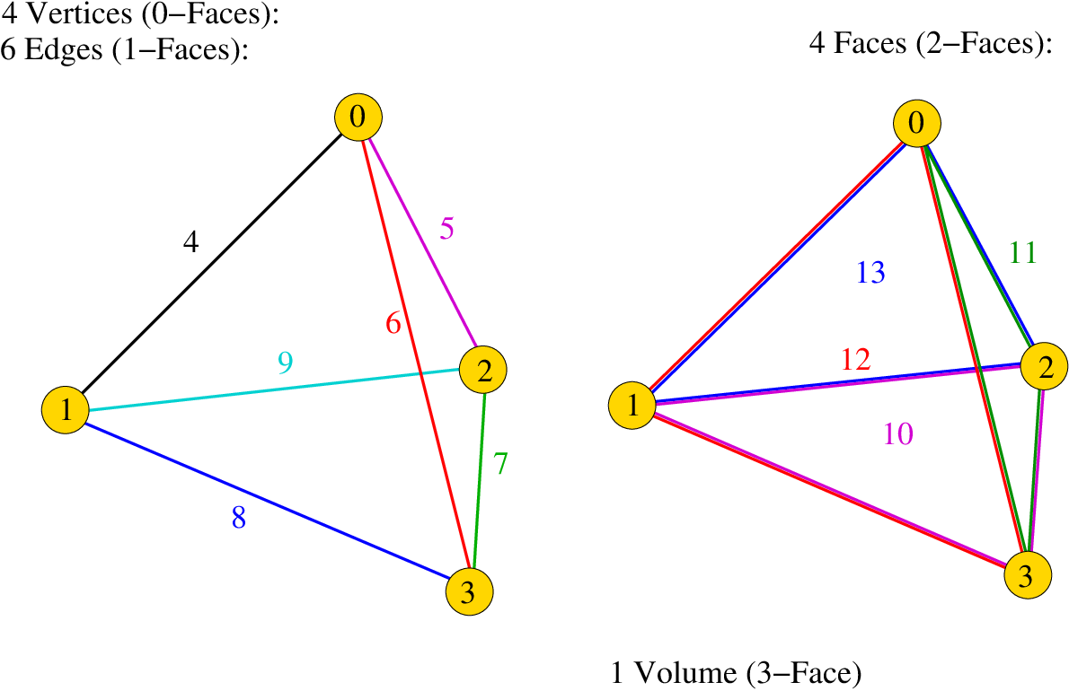
References

[1] Erwin Schrödinger; Space-Time Structure, Cambridge University Press (1950), ISBN 0-521-31520-4.
[2] Vadim Kaplunovsky and Marvin Weinstein “Space-time: Arena or Illusion?”; Phys. Rev. D 31 (1985) p. 1879. See also SLAC-PUB-3156.
[3] Yu. F. Pirogov “Spacetime Symplectic Extension”; Physics of Atomic Nuclei, Vol. 66, No. 1, (2003) pp. 135-142. From: Yadernaya Fizika, Vol. 66, No. 1, 2003, pp. 138-145.
[4] Yu. F. Pirogov “Space-time revisited”; Proc. of Quarks 2004, arxiv:gr-qc/0409067; see also: www.slac.stanford.edu/econf/C0405241.
[5] Yu. F. Pirogov “Space-time: emerging vs. existing”; (2005) arxiv:gr-qc/0503091v1.
[6] A.R. Marlow: “Quantum Theoretical Origin of Spacetime Structure”; Int. J. of Theor. Phys., Vol. 25, No. 5 (1986), pp. 561-571, and references therein.
[7] A.L.L. Videira, A.L. Rocha Barros and N.C. Fernandez “Geometry as an Aspect of Dynamics”; Found. of Phys., Vol. 15, No. 12 (1985), pp. 1247-1262.
[8] G. Amelino-Camelia, L. Freidel, J. Kowalski-Glikman and Lee Smolin “Principle of relative locality”; (arXiv:1101.0931v2) Phys. Rev. D 84, 084010.
[9] W. Smilga “Emergence of Space-Time and Gravitation”; J. of Mod. Phys. 4 (2013), 963-967; DOI: 10.4236/jmp.2013.47129.
[10] B.J. Hiley “Process, Distinction, Groupoids and Clifford Algebras: an Alternative View of the Quantum Formalism” in: Bob Coecke (Ed.), Lecture Notes in Physics Vol. 813; Springer Heidelberg Dordrecht London New York 2011.
[11] N. Seiberg, “Emergent Spacetime” in: The Quantum Structure of Space and Time, eds. D. Gross, M. Henneaux, and A. Sevrin, (World Scientific, 2007), pp. 163-213.
[12] Kevin H. Knuth and Newshaw Bahreyni “A potential foundation for emergent space-time”; J. of Math. Phys. 55 (2014), 112501.
[13] Philipp A. Höhn and Markus P. Müller “An operational approach to spacetime symmetries: Lorentz transformations from quantum communication”; arXiv:1412.8462;
[14] E.C.G. Stueckelberg “Quantum Theory in real Hilbert-Space”; Helv. Phys. Acta 33 (1960), pp. 727-752.
[15] John P. Ralston “Berry’s phase and the symplectic character of quantum time evolution”; Phys. Rev. A 40 No. 9 (1989), pp. 4872-4884.
[16] N. Buric “Hamiltonian quantum dynamics with separability constraints”; Ann. Phys. 323, 17-22 (2008).
[17] Dorje C. Brody, Anna C.T. Gustavsson and Lane P. Hughston “Symplectic approach to quantum constraints”; J. Phys. A: Math. Theor. 41 (2008) 475301.
[18] Anna C.T. Gustavsson “Constrained quantum dynamics”; Fourth International Workshop DICE2008 Journal of Physics: Conference Series 174 (2009) 012025.
[19] Hans-Thomas Elze “Linear dynamics of quantum-classical hybrids”; Phys. Rev. A 85, 052109 (2012).
[20] John S. Briggs and Alexander Eisfeld “Coherent quantum states from classical oscillator amplitudes”; Phys. Rev. A 85, 052111 (2012).
[21] John S. Briggs and Alexander Eisfeld “Quantum dynamics simulation with classical oscillators”; Phys. Rev. A 88, 062104 (2013).
[22] Thomas E. Skinner “Exact mapping of the quantum states in arbitrary N-level systems to the positions of classical coupled oscillators”; Phys. Rev. A 88, 012110 (2013).
[23] Earl T. Campbell, Marco G. Genoni and Jens Eisert “Continuous-variable entanglement distillation and noncommutative central limit theorems”; Phys. Rev. A 87, 042330 (2013).
[24] N. Buric, D.B. Popovic and M. Radonjic “Phase space theory of quantum–classical systems with nonlinear and stochastic dynamics”; Ann. Phys. 343 (2014), pp. 16-26.
[25] Mario Radovan; “On the nature of time”, arXiv:1509.01498.
[26] A. Einstein; Autobiographical Notes. Open Court Publishing, La Salle, Illinois 1996.
[27] Christian de Ronde: “Representational Realism, Closed Theories and the Quantum to Classical Limit”, this Volume (Quantum Structural Studies: Classical Emergence from the Quantum Level, Eds: Ruth E Kastner, Jasmina Jeknic-Dugic, George Jaroszkiewicz, World Scientific, 2017, ISBN: 978-1-78634-140-2).
[28] Horst Czichos, Tetsuya Saito, Leslie Smith (Eds.): Springer Handbook of Metrology and Testing, 2nd. Ed., Springer, Berlin, Heidelberg (2011), page 3.
[29] Eugene Wigner “The Unreasonable Effectiveness of Mathematics in the Natural Sciences”; Communications in Pure and Applied Mathematics, vol. 13, No. I (February 1960).
[30] W.R. Hamilton “Theory of Conjugate Functions, or Algebraic Couples; with a Preliminary and Elementary Essay on Algebra as the Science of Pure Time”; The Transactions of the Royal Irish Academy, Vol. 17 (1831), pp. 293-423. Published by: Royal Irish Academy, Stable URL: http://www.jstor.org/stable/30078796.
[31] Peter Ohrstrom “W. R. Hamilton’s View of Algebra as the Science of Pure Time and His Revision of This View”; Historia Mathematica 12 (1985), pp. 45-55.
[32] A.J. Dragt, F. Neri and G. Rangarajan “General moment invariants”; Phys. Rev. A 45 No. 4 (1992), pp. 2572-2585.
[33] Sebastian Fortin and Olimpia Lombardi: “A top-down view of the classical limit of quantum mechanics”, this Volume (Quantum Structural Studies: Classical Emergence from the Quantum Level, Eds: Ruth E Kastner, Jasmina Jeknic-Dugic, George Jaroszkiewicz, World Scientific, 2017, ISBN: 978-1-78634-140-2).
[34] Valia Allori: “Primitive Ontology and the Classical World”, this Volume (Quantum Structural Studies: Classical Emergence from the Quantum Level, Eds: Ruth E Kastner, Jasmina Jeknic-Dugic, George Jaroszkiewicz, World Scientific, 2017, ISBN: 978-1-78634-140-2).
[35] E.T. Jaynes “Scattering of Light by Free Electrons as a Test of Quantum Theory” in: The Electron, Eds. D. Hestenes and A. Weingartshofer. Kluwer Academic Publishers (1991).
[36] Concerning complex numbers we follow the notion of D. Hestenes: Imaginary numbers are not real and we demand that the unit imaginary might be convenient but is not required in the formulation of a physical theory. See also: S. Gull, A. Lasenby, C. Doran “Imaginary numbers are not real - The geometric algebra of spacetime”; Found. of Phys. Vol. 23, Issue 9 (1993), 1175-1201.
[37] Martin Erik Horn “Living in a world without imaginaries”; Journal of Physics: Conference Series 380 (2012) 012006.
[38] Gary W. Gibbons in: The Arrows of Time, Fundamental Theories of Physics 172; Springer Berlin Heidelberg 2012.
[39] K. Zare and V. Szebehely “Time transformations in the extended phase-space”; Cel. Mech. Vol. 11 (1975), pp. 469-482.
[40] Sergio Blanes and Chris J. Budd “Explicit Adaptive Symplectic (EASY) Integrators: A Scaling Invariant Generalization of the Levi-Civita and KS Regularizations”; Celest. Mech. and Dyn. Astron. 89 (2004), 383-405.
[41] See theorem 3.2.1. in Ref. [42].
[42] K.R. Meyer, G.R. Hall and D. Offin; Introduction to Hamiltonian Dynamical Systems and the N-Body Problem; 2nd. Ed., Springer (2000).
[43] Richard Becker Theory of Heat, 2nd Ed.: Springer Berlin, Heidelberg, New York 1967.
[44] Y.S. Kim and M.E. Noz Phase Space Picture of Quantum Mechanics; World Scientific, Singapore, New Jersey, London, Hongkong (1991).
[45] Peter D. Lax “Integrals of Nonlinear Equations of Evolution and Solitary Waves”; Courant Inst. (N.Y. Univ.), Rep. NYO-1480-87 (1968); also in: Comm. Pure Appl. Math. Vol. 21, No. 5 (1968), pp. 467-490.
[46] Jose F. Carinena, Alberto Ibort, Guiseppe Marmo and Guiseppe Morandi Geometry from Dynamics, Classical and Quantum; Springer 2015, p. 558.
[47] W.-H. Steeb and A. Kunick; Chaos in dynamischen Systemen, B.I. Wissenschaftsverlag, Mannheim/Wien/Zürich (1989), 2nd ed. (in German).
[48] C. Baumgarten “Use of real Dirac matrices in two-dimensional coupled linear optics”; Phys. Rev. ST Accel. Beams. 14, 114002 (2011).
[49] C. Baumgarten “Geometrical method of decoupling”; Phys. Rev. ST Accel. Beams. 15, 124001 (2012).
[50] I. M. Belen’kii “A method of regularizing the equations of motion in the central force field”; Cel. Mech. 23 (1981), pp. 9-23.
[51] C. Baumgarten “A Symplectic Method to Generate Multivariate Normal Distributions”; arXiv:1205.3601.
[52] Emile Grgin and Aage Petersen “Duality of observables and generators in classical and quantum mechanics”; J. Math. Phys. Vol. 15 No. 6 (1974), 764-769.
[53] This definition holds only for a flat spacetime. In curved spacetime, this definition would have to be modified; in spherical trigonometry the theorem of Pythagoras also has to be replaced by the rules of John Napier.
[54] Ernst Binz, Maurice A. de Gosson and Basil J. Hiley “Clifford Algebras in Symplectic Geometry”; Found. of Phys. Vol. 43 (2013) 424-439.
[55] H. Bacry and M. Boon “Boson algebra as a symplectic Clifford algebra”; J. Math. Phys. 28 (1987), 2639-2649.
[56] C. Baumgarten “A new look at linear (non-?) symplectic ion beam optics in magnets”; Nucl. Instr. Meth. A 735 (2014) 546-551.
[57] Susumu Okubo “Real representations of finite Clifford algebras”; J. Math. Phys. 32, (1991), 1657-1668.
[58] Igor F. Herbut, “Majorana mass, time reversal symmetry, and the dimension of space”, Phys. Rev. D 87, 085002 (2013).
[59] G. Nibart “Building the SpaceTime Structure in Theories of Physics”; AIP Conference Proceedings 839, (2006) 198; doi: 10.1063/1.2216629.
[60] Dai-Ning Cho and Otto C.W. Kong “Relativity symmetries and Lie algebra contractions”; Annals of Physics 351 (2014), pp. 275-289.
[61] Dae-Gyu Lee “The Dirac gamma matrices as “relics” of a hidden symmetry?: As fundamental representations of the algebra sp(4,R)”; J. Math. Phys. 36 (1995), 524-530.
[62] P.A.M. Dirac “A Remarkable Representation of the 3 + 2 de Sitter Group”; J. Math. Phys. Vol. 4, Issue 7 (1963), 901-909.
[63] Ettore Majorana “Teoria simmetrica dell’elettrone e del positrone” (“A symmetric theory of electrons and positrons”); Il Nuovo Cimento 5 (1937), 171-184.
[64] W. Pauli, “Contributions mathematiques a la theorie des matrices de Dirac”. Ann. Inst. Henri Poincare 6, (1936), pp. 109-136.
[65] K. Scharnhorst “A special irreducible matrix representation of the real Clifford algebra C(3,1)”; J. of Math. Phys. 40, No. 7 (1999).
[66] D. Hestenes Space-Time Algebra; Gordon and Breach, New York, 1966). See also: arXiv:0802.2728v1.
[67] James M. Chappell, Azhar Iqbal, Derek Abbott “Geometric Algebra: A natural representation of three-space”; (2011) arXiv:1101.3619v2.
[68] See for instance (in German) P. Schmüser: Feynman-Graphen und Eichtheorien für Experimentalphysiker; Lecture Notes in Physics No. 295, Springer 1988.
[69] N.D. Mermin “Relativity without light”; Am. J. Phys. Vol. 52 Issue 2 (1984), 119-124.
[70] Sardar Singh “Lorentz transformations in Mermin’s relativity without light”; Am. J. Phys. Vol. 54 Issue 2 (1986), 183-184.
[71] R. Penrose and W. Rindler Spinors and Spacetime; Cambridge University Press 1984.
[72] R.P. Feynman, R.B. Leighton and M. Sands; Lecture Notes in Physics (Addison-Wesley Publ. Co., Inc., Reading, Mass. 1964), Vol. 2, p.26-2; http://feynmanlectures.caltech.edu/.
[73] J.M. Jauch and F. Rohrlich The Theory of Photons and Electrons; 2nd Ed., Springer (1976).
[74] Edward J. Gillis; “Relativity Is Not About Spacetime” (2012); arXiv:1210.3575.
[75] Eric P. Verlinde “On the Origin of Gravity and the Laws of Newton”; JHEP 1104:029,2011 (arXiv:1001.0785).
[76] Nima Lashkari, Michael B. McDermott, Mark Van Raamsdonk “Gravitational Dynamics From Entanglement T̈hermodynamics’̈’; JHEP 1404 (2014) 195, and arXiv:1308.3716.
[77] A. Einstein Relativity: The Special and the General Theory; 15th Edt., Appendix V (Crown Publishers - Bonanza Books, N.Y., 1961).
[78] E. Krefetz “D̈erivationöf Maxwell’s Equations”; Am. J. Phys. Vol. 38, No. 4 (1970), pp. 513-516.
[79] D.H. Kobe “Derivation of Maxwell’s equations from the local gauge invariance of quantum mechanics”; Am. J. Phys. Vol. 46, No. 5 (1978), pp. 342-348;
[80] D.H. Kobe “Derivation of Maxwell’s equations from the gauge invariance of classical mechanics”; Am. J. Phys. Vol. 48, No. 4 (1980), pp. 348-353.
[81] Freeman J. Dyson “Feynman’s proof of the Maxwell equations”; Am. J. Phys. Vol. 58, No. 3 (1990), pp. 209-214.
[82] A. Gersten “Euclidean Special Relativity”; Found. Phys. Lett. Vol. 12, No. 3 (1999), pp. 291-298.
[83] G. Diener, J. Weissbarth, F. Grossmann and R. Schmidt “Obtaining Maxwell’s equations heuristically”; Am. J. Phys. Vol. 81, No.2 (2013), pp.120-123.
[84] M. Gromov “Pseudo holomorphic curves in symplectic manifolds”; Inventiones mathematicae Vol. 82, Issue 2, (1985) pp. 307-347.
[85] Maurice A. de Gosson “The Symplectic Egg”; arXiv:1208.5969.
[86] Juan A. Mignaco “Electromagnetic Duality, Charges, Monopoles, Topology,…”; Braz. J. of Phys., Vol. 31, No. 2 (2001), pp. 235-246.
[87] Lindsey J. Leblanc “Magnetic monopoles — particles carrying a single magnetic charge — have never been seen. Analogues of these entities have now been produced in an ultracold cloud of rubidium atoms.”; Nature Vol. 505 (2014), pp. 627-628; and M. W. Ray, E. Ruokokoski, S. Kandel, M. Möttönen and D. S. Hall “Observation of Dirac monopoles in a synthetic magnetic field”, ibid. pp. 657-666.
[88] John P. Ralston “Quantum Theory without Planckś Constant”; arXiv:1203.5557.
[89] L. Hsu and J.P. Hsu “The physical basis of natural units and truly fundamental constants”; Eur. Phys. J. Plus (2012) 127: 11.
[90] M.J. Duff “How fundamental are fundamental constants?”; arXiv:1412.2040v1.
[91] Max Tegmark: “The Mathematical Universe” (2007); arXiv:0704.0646.
[92] Ikuo S. Sogami “Extended Standard Model in multi-spinor field formalism: Visible and dark sectors”; Prog. Theor. Exp. Phys. 2013, 123B02. See also: “Generalized Dirac Equation with Four Orthogonal Families of Spin 1/2 Solutions”, Prog. Theor. Phys. 66 (1981), pp. 303-317 and “New Algebraic Unified Theory of Leptons and Quarks” in Prog. Theor. Phys. 78 (1987), p. 487-505.
[93] D. Hestenes “Spacetime physics with geometric algebra”; Am. J. Phys. Vol. 71, Issue 7 (2003), 691-741.
[94] In this respect it might also be worth mentioning the applications of Clifford algebraic methods in robot vision tasks. See for instance: E. Baryo-Corrochano “What Can Hamilton, Grassmann, Clifford and Hestenes Tell us About Perception and Action Systems”; Adv. appl. Clifford alg. 20 (2010), pp. 217-240.
[95] Mark Van Raamsdonk in: Z. Merali “The Origins of Space and Time”; Nature Vol. 500 (2013), 516-519.
[96] A. Hurwitz “Über die Komposition der quadratischen Formen von beliebig vielen Variablen” (in German); Math. Ann. 88 (1923), pp. 1-25.
[97] P. Kustaanheimo and E. Stiefel “Perturbation theory of Kepler motion based on spinor regularization”; J. reine ang. Math. Vol. 1965, Issue 218 (1965), 204-219.
[98] M.D. Shuster “A Survey of Attitude Representations”; The Journal of the Astronautical Sciences Vol. 41, No. 4 (1993) 439-517; ibd.: Vol. 56, No. 3 (2008), pp. 359-373.
[99] See for instance: L.C. Davtyan, L.G. Mardoyan, G.S. Pogosyan, A.N. Sissakian and V.M. Ter-Antonyan “Generalized KS transformation: from five-dimensional hydrogen atom to eight-dimensional isotrope oscillator”; J. Phys. A: Math. Gen. Vol. 20 (1987), pp. 6121-6125 and references therein.
[100] Roger A. Horn and Charles R. Johnson, Matrix Analysis; Cambridge University Press 1985.
[101] A. J. MacFarlane “Dirac Matrices and the Dirac Matrix Description of Lorentz Transformations”; Commun. math. Phys. 2 (1966), 133-146.
[102] David M Goodmanson “A graphical representation of the Dirac algebra”; Am. J. Phys. 64 (7), 1996, pp. 870-880. Preprint: arXiv:hep-th/0612148.

Minkowski Spacetime and QED from Ontology of Time

Abstract

Keywords:

pacs

I Introduction

I.1 Spacetime vs. Proper Time

I.2 The Form of Physics

I.3 Outline

II Obligations of a Fundamental Theory

III Variables, Constants and the Hamiltonian

III.1 Variables

III.2 The Hamiltonian

IV Constants of Motion

IV.1 Measurable Quantities: Observables

V From Lie Algebra to Spacetime Geometry

VI Structure Preservation

VI.1 Transfer Matrizes and Symplectic Transformations

VI.2 Time-Dependent Hamiltonian

VI.3 Cosymplices as Generators of Transformations

VII The Dimensionality of Spacetime

VII.1 Clifford Algebras

VII.2 The Number of Space Dimensions

VII.3 The Real Dirac Matrices

VIII Lorentz Transformations are Symplectic Transformations

VIII.1 The Electromechanical Equivalence (EMEQ)

VIII.2 The Lorentz Force

IX Electrodynamics from Symplectic Spacetime

IX.1 The Density

IX.2 The Wave Equations

IX.3 Lightlike Spinors and massive Multispinors

IX.4 Deformation of the Phase Space Unit Cell

IX.5 CPT-Transformations

IX.6 Duality between Operators and Observables

X Anything Else?

X.1 Once More: Cosymplices

X.2 Higher-Dimensional Spaces

XI Summary and Conclusion

Acknowledgements.

Appendix A Hurwitz and Kustaanheimo-Stiefel Matrices

Appendix B Arbitrary constant Hamiltonians

Appendix C (Co-) Symplices for higher-dimensional Spacetimes

C.1 Which kk-Vectors are (Co-) Symplices

C.2 The real Pauli matrices and the structure of (co-) symplices for nn DOFs

C.3 Which kk-Vectors of C​lN−1,1Cl_{N-1,1} are (Anti-) Symmetric

Appendix D The Kustaanheimo-Stiefel Transformation

Appendix E Non-Symplectic Transformations

E.1 Simple LC-Circuit

E.2 Coupled LC-Circuits

E.3 The Direction of Time

E.4 Nonsymplectic Transformations within the Dirac Algebra

E.5 Transformation to the Conventional Dirac Algebra

Appendix F Graphical Representation of Dirac Matrices

References

References

C.1 Which $k$ -Vectors are (Co-) Symplices

C.2 The real Pauli matrices and the structure of (co-) symplices for $n$ DOFs

C.3 Which $k$ -Vectors of $Cl_{N-1,1}$ are (Anti-) Symmetric