On Milnor fibrations of mixed functions, $a_{f}$ -condition and boundary stability

Mutsuo Oka Address: Department of Mathematics Tokyo University of Science 1-3, Kagurazaka, Shinjuku-ku Tokyo 162-8601 g E-mail: oka@rs.kagu.tus.ac.jp

Abstract.

Convenient mixed functions with strongly non-degenerate Newton boundaries have a Milnor fibration ([9]), as the isolatedness of the singularity follows from the convenience. In this paper, we consider the Milnor fibration for non-convenient mixed functions We also study geometric properties such as Thom’s $a_{f}$ condition, the transversality of the nearby fibers and stable boundary property of the Milnor fibration and their relations.

Key words and phrases:

Mixed function,

a_{f}

- condition, Milnor fibration

2000 Mathematics Subject Classification

14J70,14J17, 32S25

1. Preliminary

Let $f(\mbox{\bf z},\bar{\mbox{\bf z}})$ be a mixed function and write it as sum of real and imaginary part: $f=g+ih$ . Writing $\mbox{\bf z}=(z_{1},\dots,z_{n})$ and $z_{j}=x_{j}+iy_{j}\,(j=1,\dots,n)$ with $x_{j},y_{j}\in\mathbb{R}$ , the mixed hypersurface $\{f=0\}$ can be understand as the real analytic variety in $\mathbb{R}^{2n}$ defined by $\{g=h=0\}$ . The real and imaginary part $g,h$ are also (real-valued) mixed functions and we also consider them as real analytic functions of variables $\mbox{\bf x}=(x_{1},\dots,x_{n})$ and $\mbox{\bf y}=(y_{1},\dots,y_{n})$ . By abuse of notations we use both notations $g(\mbox{\bf z},\bar{\mbox{\bf z}})$ and $g(\mbox{\bf x},\mbox{\bf y})$ etc. We recall some notations. The real gradient vector for a real-valued mixed function $k(\mbox{\bf x},\mbox{\bf y})$ is defined as

(1)		$\displaystyle{\rm{grad}\/}\,k$	$\displaystyle=$	$\displaystyle({\rm{grad}\/}_{\mbox{\bf x}}k,{\rm{grad}\/}_{\mbox{\bf y}}k)\in\mathbb{R}^{2n}$
(2)		$\displaystyle{\rm{grad}\/}_{\mbox{\bf x}}k$	$\displaystyle=$	$\displaystyle(k_{x_{1}},\dots,k_{x_{n}}),\,\,{\rm{grad}\/}_{\mbox{\bf y}}k=(k_{y_{1}},\dots,k_{y_{n}}).$

Here $k_{x_{i}},k_{y_{j}}$ are respective partial derivatives. $\mathbb{C}^{n}$ and $\mathbb{R}^{2n}$ are identified by $\mbox{\bf z}\leftrightarrow\mbox{\bf z}_{\mathbb{R}}=(\mbox{\bf x},\mbox{\bf y})$ . Under this identification, the Euclidean inner product in $\mathbb{R}^{2n}$ (denoted as $(*,*)_{\mathbb{R}}$ ) and the hermitian inner product in $\mathbb{C}^{n}$ (denoted as $(*,*)$ ) are related as $(\mbox{\bf z}_{\mathbb{R}},\mbox{\bf z}_{\mathbb{R}}^{\prime})_{\mathbb{R}}=\Re(\mbox{\bf z},\mbox{\bf z}^{\prime})$ . For a mixed function $k$ (not necessarily real-valued), we define also holomorphic and anti-holomorphic gradients as

\begin{split}&{\rm{grad}\/}_{\partial}k=(\frac{\partial k}{\partial z_{1}},\dots,\frac{\partial k}{\partial z_{n}}),\\ &{\rm{grad}\/}_{\bar{\partial}}k=(\frac{\partial k}{\partial\bar{z}_{1}},\dots,\frac{\partial k}{\partial\bar{z}_{n}}).\end{split}

For simplicity of notations, we use the following notations:

\begin{split}&dk:={\rm{grad}\/}\,k,\,\,d_{\mbox{\bf x}}k:={\rm{grad}\/}_{\mbox{\bf x}}k,\,\,d_{\mbox{\bf y}}k:={\rm{grad}\/}_{\mbox{\bf y}}k,\,\,\\ &\partial k:={\rm{grad}\/}_{\partial}k,\,\,{\bar{\partial}}\,k:={\rm{grad}\/}_{\bar{\partial}}k.\end{split}

Note that if $k$ is real-valued,

(3)

\displaystyle\overline{\partial k}={\bar{\partial}}k,

and real vector $dk\in\mathbb{R}^{2n}$ corresponds to the complex vector $2\overline{\partial k}\in\mathbb{C}^{n}$ .

1.0.1. Tangent spaces

Let $k(\mbox{\bf z},\bar{\mbox{\bf z}})$ is a real valued mixed function. Then the tangent space of a regular point $\mbox{\bf a}\in V_{\eta}:=k^{-1}(\eta),\eta\in\mathbb{R}$ is described as follows. For a complex vector $\mbox{\bf a}\in\mathbb{C}^{n}$ , we denote the corresponding real vector as $\mbox{\bf a}_{\mathbb{R}}\in\mathbb{R}^{2n}$ .

\begin{split}T_{\mbox{\bf a}}V_{k}&=\{\mbox{\bf v}_{\mathbb{R}}\in\mathbb{R}^{2n}\,|\ (\mbox{\bf v}_{\mathbb{R}},dk(\mbox{\bf a}_{\mathbb{R}}))_{\mathbb{R}}=0\}\\ &=\{\mbox{\bf v}\in\mathbb{C}^{n}\,|\,\Re(\mbox{\bf v},\overline{\partial k}(\mbox{\bf a}))=0\}.\end{split}

Consider the mixed hypersurface $V_{\eta}=f^{-1}(\eta),\,\eta\neq 0$ . We introduce two vectors in $\mathbb{C}^{n}$ which are more convenient to describe the Milnor fibration of the first type:

\begin{split}&\mbox{\bf v}_{1}:=\overline{\partial f}(\mbox{\bf z},\bar{\mbox{\bf z}})+\bar{\partial}f(\mbox{\bf z},\bar{\mbox{\bf z}}),\\ &\mbox{\bf v}_{2}:=i(\overline{\partial f}(\mbox{\bf z},\bar{\mbox{\bf z}})-\bar{\partial}f(\mbox{\bf z},\bar{\mbox{\bf z}})).\end{split}

These vectors describe the respective tangent spaces at a regular point a of the real codimension 1 varieties

\begin{split}&V_{1}:=\{\mbox{\bf z}\,|\,|f(\mbox{\bf z},\bar{\mbox{\bf z}})|=|f(\mbox{\bf a},\bar{\mbox{\bf a}})|\},\\ &V_{2}:=\{\mbox{\bf z}\,|\,\arg\,f(\mbox{\bf z},\bar{\mbox{\bf z}})=\arg\eta\}.\end{split}

Namely, we have shown (Lemma 30,Observation 32,[9])

\begin{split}&T_{\mbox{\bf a}}V_{1}:=\{\mbox{\bf v}\,|\,\Re(\mbox{\bf v},\mbox{\bf v}_{1}(\mbox{\bf a}))=0\}\\ &T_{\mbox{\bf a}}V_{2}:=\{\mbox{\bf v}\,|\,\Re(\mbox{\bf v},\mbox{\bf v}_{2}(\mbox{\bf a}))=0\}.\end{split}

Note that $V_{\eta}=V_{1}\cap V_{2}$ . Observe that the two subspaces of dimension two

<\bar{\partial}g(\mbox{\bf a},\bar{\mbox{\bf a}}),\bar{\partial}h(\mbox{\bf a},\bar{\mbox{\bf a}})>_{\mathbb{R}},\,<\mbox{\bf v}_{1}(\mbox{\bf a}),\mbox{\bf v}_{2}(\mbox{\bf a})>_{\mathbb{R}}

are equal. In fact we have:

	$\displaystyle\mbox{\bf v}_{1}$	$\displaystyle=$	$\displaystyle\frac{\overline{\partial f}}{\bar{f}}+\frac{\bar{\partial}f}{f}=\frac{1}{\|f\|^{2}}(f(\overline{\partial g}-i\overline{\partial h})+\bar{f}(\bar{\partial}g+i\bar{\partial}h))=\frac{1}{\|f\|^{2}}(2g\bar{\partial}g+2h\bar{\partial}h)$
	$\displaystyle\mbox{\bf v}_{2}$	$\displaystyle=$	$\displaystyle i\frac{\overline{\partial f}}{\bar{f}}+\frac{\bar{\partial}f}{f}=\frac{i}{\|f\|^{2}}(f(\bar{\partial}g-i\bar{\partial}h)+\bar{f}(\bar{\partial}g+i\bar{\partial}h))=\frac{1}{\|f\|^{2}}(-2h\bar{\partial}g-2g\bar{\partial}h)$

Proposition 1.

([8]) Put $f=g+hi$ as before. The next conditions are equivalent.

(1)

$\mbox{\bf a}\in\mathbb{C}^{n}$ is a critical point of the mapping $f:\mathbb{C}^{n}\to\mathbb{C}$ .
(2)

$dg(\mbox{\bf a}_{\mathbb{R}}),\,dh(\mbox{\bf a}_{\mathbb{R}})$ are linearly dependent over $\mathbb{R}$ .
(3)

$\bar{\partial}g(\mbox{\bf a},\bar{\mbox{\bf a}}),\,\bar{\partial}h(\mbox{\bf a},\bar{\mbox{\bf a}})$ are linearly dependent over $\mathbb{R}$ .
(4)

There exists a complex number $\alpha$ with $|\alpha|=1$ such that $\overline{\partial f}(\mbox{\bf a},\bar{\mbox{\bf a}})=\alpha\,\bar{\partial}f(\mbox{\bf a},\bar{\mbox{\bf a}})$ .

Under the above equivalent conditions, we say that a is a mixed singular point of the mixed hypersurface $f^{-1}(f(\mbox{\bf a}))$ .

Lemma 2.

(cf [3]) Put $V_{\eta}=f^{-1}(\eta)$ and take $\mbox{\bf p}\in S_{r}\cap V_{\eta}$ . Assume that p is a non-singular point of $V_{\eta}$ and let $k(\mbox{\bf z},\bar{\mbox{\bf z}})$ be a real valued mixed function. The following conditions are equivalent.

(1)

The restriction $k|V_{\eta}$ has a critical point at $\mbox{\bf a}\in V_{\eta}$ .
(2)

There exists a complex number $\alpha\in\mathbb{C}^{*}$ such that $\bar{\partial}k(\mbox{\bf p})=\alpha\overline{\partial f}(\mbox{\bf p},\bar{\mbox{\bf p}})+\bar{\alpha}\bar{\partial}f(\mbox{\bf p},\bar{\mbox{\bf p}})$ .
(3)

There exist real numbers $c,d$ such that

$\bar{\partial}k(\mbox{\bf p})=c\bar{\partial}g(\mbox{\bf p},\bar{\mbox{\bf p}})+d\bar{\partial}h(\mbox{\bf p},\bar{\mbox{\bf p}}).$

(4)

There exist real numbers $c^{\prime},d^{\prime}$ such that

\bar{\partial}k(\mbox{\bf p})=c^{\prime}\bar{\mbox{\bf v}}_{1}(\mbox{\bf p},\bar{\mbox{\bf p}})+d^{\prime}\mbox{\bf v}_{2}(\mbox{\bf p},\bar{\mbox{\bf p}}).

Proof.

As $\mbox{\bf p}\in V$ is assumed a non-singular point, (1) and (3) are equivalent. We show the implication (3) $\implies$ (2). Assume

\bar{\partial}k(\mbox{\bf p})=c\,\bar{\partial}g(\mbox{\bf p},\bar{\mbox{\bf p}})+d\,\bar{\partial}h(\mbox{\bf p},\bar{\mbox{\bf p}}),\quad\exists c,d\in\mathbb{R}.

We use the equality:

(4)			$\displaystyle\bar{\partial}g(\mbox{\bf p},\bar{\mbox{\bf p}})$	$\displaystyle=\frac{\bar{\partial}f(\mbox{\bf p},\bar{\mbox{\bf p}})+\overline{\partial f}(\mbox{\bf p},\bar{\mbox{\bf p}})}{2},$
(5)			$\displaystyle\bar{\partial}h(\mbox{\bf p},\bar{\mbox{\bf p}})$	$\displaystyle=\frac{i(\bar{\partial}f(\mbox{\bf p},\bar{\mbox{\bf p}})-\overline{\partial f}(\mbox{\bf p},\bar{\mbox{\bf p}}))}{2}$

to obtain the equality:

\bar{\partial}k(\mbox{\bf p})=\frac{c-di}{2}\bar{\partial}f(\mbox{\bf p},\bar{\mbox{\bf p}})+\frac{c+di}{2}\overline{\partial f}(\mbox{\bf p},\bar{\mbox{\bf p}}).

The implication $(2)\to(3)$ can be shown similarly, using the equality

(6)

\displaystyle\partial f=\partial g+i\partial h,\bar{\partial}f=\bar{\partial}g+i\bar{\partial}h

∎

1.0.2. Newton boundary and strong non-degeneracy condition.

Let $f(\mbox{\bf z},\bar{\mbox{\bf z}})=\sum_{\nu,\mu}c_{\nu\mu}\mbox{\bf z}^{\nu}{\bar{\mbox{\bf z}}}^{\mu}$ be a mixed polynomial. The Newton polygon $\Gamma_{+}(f)$ is defined by the convex hull of $\bigcup(\nu+\mu+\mathbb{R}_{+}^{n})$ where the sum is taken for $\nu,\mu$ with $c_{\nu\mu}\neq 0$ . Newton boundary $\Gamma(f)$ is the union of compact faces of $\Gamma_{+}(f)$ as usual. $f$ is called convenient if for any $i=1,\dots,n$ , $\Gamma(f)$ intersects with $z_{i}$ -axis. To treat the case of non-convenient functions, we define the modified Newton boundary $\Gamma_{nc}(f)$ by adding essential non-compact faces $\Xi$ . Here $\Xi$ is called an essential non-compact face if there exists a semi-positive weight vector $P={}^{t}(p_{1},\dots,p_{n})$ such that

(1)

$\Delta(P)=\Xi$ with $\Xi$ being a non-compact face and $f^{I(P)}\equiv 0$ where $I(P)=\{i\,|\,p_{i}=0\}$ and
(2)

for any $i\in I(P)$ and any point $\nu\in\Xi$ , the half line starting from $\nu$ , $\nu+\mathbb{R}_{+}E_{i}$ is contained in $\Xi$ . Here $E_{i}$ is the unit vector in the direction of $i$ -th coordinate axis.

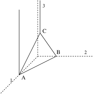
The weight vector $P$ may not unique but $I(P)$ does not depend on $P$ . Thus we denote it as $I(\Xi)$ and it is called the non compact direction of $\Xi$ . See Figure 1 which shows the modified Newton boundary of $f=z_{1}^{3}+z_{2}^{3}+z_{2}z_{3}^{2}$ in Example 3.

For any non-negative weight vector $P$ , it defines a linear function $\ell_{P}$ on $\Gamma_{+}(f)$ by $\ell_{P}(\xi)=p_{1}\xi_{1}+\cdots+p_{n}\xi_{n}$ where $P={}^{t}(p_{1},\dots,p_{n}),\,\xi=(\xi_{1},\dots,\xi_{n})\in\Gamma(f)$ and the minimal value is denoted as $d(P)$ and the face where this minimal value is taken is denoted by $\Delta(P)$ . In other word, $\Delta(P):=\{\xi\in\Gamma_{nc}(f)\,|\,\sum_{i=1}^{n}p_{i}\xi_{i}=d(P)\}$ . The face function associated by $P$ is defined as $f_{P}:=f_{\Delta(P)}$ .

$f$ is called strongly non-degenerate if (1) for any compact face $\Delta\subset\Gamma_{nc}(f)$ , the face function $f_{\Delta}:=\sum_{\nu+\mu\in\Delta}c_{\nu\mu}\mbox{\bf z}^{\nu}{\bar{\mbox{\bf z}}}^{\mu}$ has no critical point as a function $f_{\Delta}:\mathbb{C}^{*n}\to\mathbb{C}$ and (2) for a non-comact face $\Delta\in\Gamma_{nc}(f)$ , $f_{\Delta_{0}}:\mathbb{C}^{*n}\to\mathbb{C}$ has no critical point where $\Delta_{0}=\Delta\cap\Gamma(f)$ .

Example 3.

Consider a holomorphic function $f=z_{1}^{3}+z_{2}^{3}+z_{2}z_{3}^{2}$ of three variables. Note that $\Gamma_{nc}(f)$ has three vertices $A=(3,0,0),B=(0,3,0),C=(0,1,2)$ and the face $\Delta:=\{\overline{AC}+\mathbb{R}_{+}\,E_{3}\}\subset\Gamma_{nc}(f)$ where $\overline{AC}$ is the edge with endpoints $A,C$ . The non-compact faces with edge $\overline{AB}$ and $\overline{BC}$ are not essential. They are not vanishing coordinates i.e., $f$ does not vanish on $\{z_{1}=z_{3}=0\}$ or $\{z_{2}=z_{3}=0\}$ . See Figure 1.

Refer to caption — Figure 1. $Non-compactface$

2. Milnor fibration

Asume that $f(\mbox{\bf z},\bar{\mbox{\bf z}})=\sum_{\nu,\mu}c_{\nu\mu}\mbox{\bf z}^{\nu}{\bar{\mbox{\bf z}}}^{\mu}$ is a strongly non-degenerate mixed polynomial and let $V=f^{-1}(0)$ . In this section, we study the Milnor fibration of $f$ . If $f(\mbox{\bf z},\bar{\mbox{\bf z}})$ has a convenient Newton boundary, the singularity is isolated and there exists a spherical Milnor fibration (= a Milnor fibrations of the first type):

f/|f|:S_{r}-K\to S^{1},\quad K=V\cap S_{r}

and also a tubular Milnor fibration (= Milnor fibration of the second type): $f:\partial E(r,\delta)^{*}\to S_{\delta}^{1}$ where $\partial E(r,\delta)^{*}=\{\mbox{\bf z}\in B_{r}\,|\,|f(\mbox{\bf z},\bar{\mbox{\bf z}})|=\delta\}$ for sufficiently small $r,\delta$ such that $0<\delta\ll r$ . They are $C^{\infty}$ -equivalent (Theorems 19, 33, 37,[9]).

For non-convenient mixed function, the singularity need not be isolated. We have proved the same assertion under an extra condition “super strongly non-degenerate” (Theorem 52,[9]). In this paper, we prove the existence of Milnor fibrations for any strongly non-degenerate functions with a weaker assumption than the assumption “super”. We will study also some geometric properties behind the argument.

2.1. Smoothness of the nearby fibers

First we recall the following:

Lemma 4.

(Lemma 28,[9]) Assume that $f(\mbox{\bf z},\bar{\mbox{\bf z}})$ is a strongly non-degenerate mixed function. Then there exists a positive number $r_{0}$ and $\delta$ such that the fiber $V_{\eta}:=f^{-1}(\eta)$ has no mixed singularity in the ball $B_{r_{0}}^{2n}$ for any non-zero $\eta$ with $|\eta|\leq\delta$ .

Proof.

Though the proof is the same as that in [9], we repeat it for the beginner’s convenience. We show a contradiction , assuming that the assertion does not hold. Then using the Curve Selection Lemma ([6, 4]), we can find an analytic path $\mbox{\bf z}(t),\,0\leq t\leq 1$ such that $\mbox{\bf z}(0)=O$ and $f(\mbox{\bf z}(t),\bar{\mbox{\bf z}}(t))\neq 0$ and $\mbox{\bf z}(t)$ is a critical point of the function $f:{\mathbb{C}}^{n}\to{\mathbb{C}}$ for any $t\neq 0$ . Using Proposition 1, we can find a real analytic family $\lambda(t)$ in $S^{1}\subset{\mathbb{C}}$ such that

(7)

\displaystyle\overline{\partial f}(\mbox{\bf z}(t),\bar{\mbox{\bf z}}(t))=\lambda(t)\,\bar{\partial}f(\mbox{\bf z}(t),\bar{\mbox{\bf z}}(t)).

Put $I=\{j\,|\,z_{j}(t)\not\equiv 0\}$ . We may assume for simplicity that $I=\{1,\dots,m\}$ and we consider the restriction $f^{I}=f|\mathbb{C}^{I}$ . As $f(\mbox{\bf z}(t),\bar{\mbox{\bf z}}(t))=f^{I}(\mbox{\bf z}(t),\bar{\mbox{\bf z}}(t))\not\equiv 0$ , we see that $f^{I}\neq 0$ . Consider the Taylor expansions of $\mbox{\bf z}(t)$ and $\lambda(t)$ :

	$\displaystyle\mbox{\bf z}_{i}(t)=b_{i}\,t^{a_{i}}+\text{(higher terms)},\,b_{i}\neq 0,a_{i}>0,\quad i=1,\dots,m$
	$\displaystyle\lambda(t)=\lambda_{0}+\text{(higher terms)},\quad\lambda_{0}\in S^{1}\subset{\mathbb{C}}.$

Consider the weight vector $A={}^{t}(a_{1},\dots,a_{m})$ and a point in the torus $\mbox{\bf b}=(b_{1},\dots,b_{m})\in\mathbb{C}^{*I}$ and we consider the face function $f^{I}_{A}$ of $f^{I}(\mbox{\bf z},\bar{\mbox{\bf z}})$ . Then we have for $j\in I$

	$\displaystyle\frac{\partial f}{\partial z_{j}}(\mbox{\bf z}(t),\bar{\mbox{\bf z}}(t))=\frac{\partial f^{I}_{A}}{\partial z_{j}}(\mbox{\bf b},\bar{\mbox{\bf b}})\,t^{d-a_{j}}+\text{(higher terms)},$
	$\displaystyle\frac{\partial f}{\partial\bar{z}_{j}}(\mbox{\bf z}(t),\bar{\mbox{\bf z}}(t))=\frac{\partial f^{I}_{A}}{\partial z_{j}}(\bar{\mbox{\bf b}},\bar{\mbox{\bf b}})\,t^{d-a_{j}}+\text{(higher terms)}$

where $d=d(A;f^{I})$ . The equality (7) says that

{\overline{\frac{\partial f^{I}}{\partial z_{j}}}\,(\mbox{\bf z}(t),\bar{\mbox{\bf z}}(t))}=\lambda(t)\,\frac{\partial f^{I}}{\partial\bar{z}_{j}}(\mbox{\bf z}(t),\bar{\mbox{\bf z}}(t)),\,\,j=1,\dots,m.

which implies the next equality:

{\rm{ord}\/}_{t}\,{\overline{\frac{\partial f^{I}}{\partial z_{j}}}\,(\mbox{\bf z}(t),\bar{\mbox{\bf z}}(t))}={\rm{ord}\/}_{t}\,\frac{\partial f^{I}}{\partial\bar{z}_{j}}(\mbox{\bf z}(t),\bar{\mbox{\bf z}}(t)),\,\,j=1,\dots,m.

Thus we get the equality:

\overline{\partial f^{I}_{A}}(\mbox{\bf b},\bar{\mbox{\bf b}})=\lambda_{0}\,\bar{\partial}f^{I}_{A}(\mbox{\bf b},\bar{\mbox{\bf b}}),\quad\mbox{\bf b}\in{\mathbb{C}}^{*m}.

This implies that b is a critical point of $f_{A}^{I}:{\mathbb{C}}^{*I}\to{\mathbb{C}}$ , which is a contradiction to the strong non-degeneracy of $f_{A}^{I}(\mbox{\bf z},\bar{\mbox{\bf z}})$ . ∎

2.2. Vanishing coordinate subspaces and essentially non-compact face functions

We assume that $f$ is a mixed polynomial (not only mixed analytic function). We denote by $\mathcal{I}_{nv}(f)$ the set of subset $I\subset\{1,2,\dots,n\}$ such that $f^{I}\not\equiv 0$ (we denoted this set as $\mathcal{NV}(f)$ in [9]). We denote by $\mathcal{I}_{v}(f)$ the set of subset $I\subset\{1,2,\dots,n\}$ such that $f^{I}\equiv 0$ , and for $I\in\mathcal{I}_{v}(f)$ and we consider also the set of non-compact faces $\Delta\in\Gamma_{nc}(f)$ such that there exists (possibly not unique) a non-negative weight $P$ such that $\Delta(P)=\Delta$ and $I(P)=I$ .　Here $I(P)=\{i\,|\,p_{i}=0\}$ . $\mathbb{C}^{I}$ is called a vanishing coordinates subspace. Note that $\mathbb{C}^{I}\subset V$ .

Definition 5.

Take an essential non-compact face $\Delta\in\Gamma_{nc}(f)$ . Take a weight function $P$ such that $f_{P}=f_{\Delta}$ and $I(P)=I(\Delta)$ . We consider the function $\rho_{\Delta}(\mbox{\bf z}):=\sum_{j\in I(\Delta)}|z_{j}|^{2}$ . An essential non-compact face function $f_{\Delta}$ is locally tame if there exists a positive number $r_{\Delta}>0$ such that for any fixed $\{z_{j}\,|\,z_{j}\neq 0,\,j\in I(\Delta)\}$ with $\rho_{\Delta}(\mbox{\bf z})\leq r_{\Delta}^{2}$ , $f_{\Delta}$ has no critical points in $\mathbb{C}^{*I(\Delta)^{c}}$ as a mixed polynomial function of $n-|I(\Delta)|$ -variables $\{z_{k}\,|\,k\notin I(\Delta)\}$ , and we can also assume that the function $\rho_{\Delta}$ has no critical value on $V_{\Delta}^{*}$ on the interval $(0,r_{\Delta}^{2}]$ where $V_{\Delta}=f_{\Delta}^{-1}(0)\subset\mathbb{C}^{*n}$ . We say that $f$ is locally tame on the vanishing coordinate subspace $\mathbb{C}^{I}$ if any face function $f_{\Delta}$ with $I(\Delta)=I$ is locally tame. This is slightly weaker condition than ”super strongly non-degenerate” in [9].

Put $r_{I}=\min\,\{r_{\Delta}\,|\,I(\Delta)=I\}$ for $I\in\mathcal{I}_{v}(f)$ and $r_{nc}=\min\,\{r_{I}\,|\,I\in\mathcal{I}_{v}(f)\}$ . If $f$ is convenient, $r_{nc}=+\infty$ .

Remark 6.

We say that $f$ is ”super strongly non-degenrate” if we can take $r_{\Delta}=\infty$ in the above definition ([9]). For the existence of $r_{\Delta}$ , we used the fact that $f$ is a polynomial.

2.3. Smoothness on the non-vanishing coordinate subspaces

Take $I\subset\{1,\dots,n\}$ and $\mathbb{C}^{I}$ is called a non-vanishing coordinate if $f^{I}\not\equiv 0$ . The set of such subsets $I$ is denoted as $\mathcal{I}_{nv}(f)$ . Put $V^{\sharp}=\cup_{I\in\mathcal{I}_{nv}(f)}V\cap\mathbb{C}^{*I}$ . Then there exists a $r_{0}>0$ so that $V^{\sharp}$ and $V^{*I}=V\cap\mathbb{C}^{*I}$ are non-singular in the ball $B_{r_{0}}$ and for any $0<r\leq r_{0}$ , the sphere $S_{r}$ and $V^{*I}$ intersect transversely. The existence of such $r_{0}$ is shown in Theorem 16, [9].

2.4. Hamm-Lê type theorem

The following is a mixed function version of Lemma (2.1.4) (Hamm-Lê,[5]). This enable us to prove the existence of Milnor fibration with locally tame behavior assumption.

Lemma 7.

Assume that $f(\mbox{\bf z},\bar{\mbox{\bf z}})$ is a strongly non-degenerate mixed polynomial which behave locally tamely along vanishing coordinate subspaces. Put $\rho_{0}=\min\,\{r_{nc},r_{0}\}$ where $r_{nc}$ and $r_{0}$ are described above. For any fixed positive number $r_{1}\leq\rho_{0}$ , there exists positive numbers $\delta(r_{1})$ (depending on $r_{1}$ ) such that

(1)

the nearby fiber $V_{\eta}:=f^{-1}(\eta)$ has no mixed singularity in the ball $B_{\rho_{0}}^{2n}$ for any non-zero $\eta$ .
(2)

for any $\eta\neq 0,\,|\eta|\leq\delta(r_{1})$ and $r,\,r_{1}\leq r\leq\rho_{0}$ , the sphere $S_{r}$ and the nearby fiber $V_{\eta}=f^{-1}(\eta)$ intersect transversely.

Proof.

We have already proved the assertion (1) (Lemma 4). So we will prove the assertion (2). Assume that the assertion is false. By the Curve Selection Lemma, we can find a real analytic curve $\mbox{\bf z}(t)$ and a complex valued function $\alpha(t),\,0\leq t\leq 1$

(8)

\displaystyle z_{j}(t)=\alpha(t)\frac{\overline{\partial f}}{\partial z_{j}}(\mbox{\bf z}(t))+\bar{\alpha}(t)\frac{\partial f}{\partial\bar{z}_{j}}(\mbox{\bf z}(t)),\,\forall j

where $\mbox{\bf z}(t),\alpha(t)$ are expanded as

\begin{split}&z_{j}(t)=b_{j}t^{p_{j}}+\text{(higher terms)},\\ &\alpha(t)=\alpha_{0}t^{m}+\text{(higher terms)}.\end{split}

and $f(\mbox{\bf z}(t))\neq 0$ for $t\neq 0$ . Obviously $\alpha(t)\neq 0$ .

Put $K=\{i\,|\,z_{j}(t)\not\equiv 0\}$ and we consider the equality in $\mathbb{C}^{K}$ . Put $\mbox{\bf b}=(b_{j})$ and $P=(p_{j})$ , $I=\{j\in K\,|\,p_{j}=0\},\,I_{1}=K-I$ and $\Delta=\Delta(P)$ . In the following, we assume $K=\{1,\dots,n\}$ as the argument is the same.

Case 1. Assume that $I\in\mathcal{I}_{nv}(f)$ . Then $f^{I}\not\equiv 0$ and $\mbox{\bf b}\in V^{\sharp}$ . We assumed that $V^{\sharp}$ and $S_{\|\mbox{\bf b}\|}$ intersect transversely for any b, $\|\mbox{\bf b}\|\leq\rho_{0}$ and thus $S_{\|\mbox{\bf z}(t)\|}$ is also transverse to $V_{f(\mbox{\bf z}(t))}$ at $\mbox{\bf z}(t)$ for a small $t\ll 1$ which is a contradiction.

Case 2. Assume that $I\in\mathcal{I}_{v}(f)$ and so $f^{I}\equiv 0$ . In this case, $\Delta\in\Gamma_{nc}(f)$ . The above equality (8) says:

(9)

b_{j}t^{p_{j}}+\text{(higher terms)}=\left(\alpha_{0}\frac{\overline{\partial f_{\Delta(P)}}}{\partial z_{j}}(\mbox{\bf b})t^{m+d(P)-p_{j}}+\text{(higher terms)}\right)\\ +\left(\bar{\alpha}_{0}\frac{\partial f_{\Delta(P)}}{\partial\bar{z}_{j}}(\mbox{\bf b})t^{m+d(P)-p_{j}}+\text{(higher terms)}\right),\quad j\in K.

We compare the order in $t$ (=the lowest degree) of the both side. The left side has order $0$ and the order of the right side is at least $d+m-p_{j}$ for $j\notin I$ and at least $d(P)+m$ for $j\in I$ . Note that $\mbox{\bf b}\in\mathbb{C}^{*n}$ . If $d(P)+m>$ , we get a contradiction $b_{j}=0$ for $j\in I$ . If $d(P)+m<0$ , we get

0=\alpha_{0}\frac{\overline{\partial f_{\Delta(P)}}}{\partial z_{j}}(\mbox{\bf b})+\bar{\alpha}_{0}\frac{\partial f_{\Delta(P)}}{\partial\bar{z}_{j}}(\mbox{\bf b}),\,\forall j

which says b is a mixed critical point of $f_{\Delta}$ , a contradiction to the strong non-degeneracy. Thus $d(P)+m=0$ and

	$\displaystyle b_{j}$	$\displaystyle=$	$\displaystyle\alpha_{0}\frac{\overline{\partial f_{\Delta(P)}}}{\partial z_{j}}(\mbox{\bf b})+\bar{\alpha}_{0}\frac{\partial f_{\Delta(P)}}{\partial\bar{z}_{j}}(\mbox{\bf b}),\,j\in I$
	$\displaystyle 0$	$\displaystyle=$	$\displaystyle\alpha_{0}\frac{\overline{\partial f_{\Delta(P)}}}{\partial z_{j}}(\mbox{\bf b})+\bar{\alpha}_{0}\frac{\partial f_{\Delta(P)}}{\partial\bar{z}_{j}}(\mbox{\bf b}),\,j\in K-I.$

This says that the function $\rho_{\Delta}$ has a critical value $\|\mbox{\bf b}_{I}\|^{2}$ on $V_{\Delta}^{*}$ , as the gradient vector of $\rho_{\Delta}$ is given as

\bar{\partial}\rho_{\Delta}(\mbox{\bf b})=2\mbox{\bf b}_{I},\quad\mbox{\bf b}_{I}=\begin{cases}b_{i},\,\,&i\in I,\\ 0\,\,&i\notin I.\end{cases}

Here $V_{\Delta}^{*}=\{\mbox{\bf z}\in\mathbb{C}^{*n}\,|\,f_{\Delta}(\mbox{\bf z})=0\}$ . This is a contradiction on the assumption that the function $\rho_{\Delta}$ has no critical value on the interval $(0,\rho_{0}]$ , as $\|\mbox{\bf b}\|\leq\rho_{0}\leq r_{\Delta}/2$ . ∎

Remark 8.

The assertion (2) also follows from $a_{f}$ -condition (see Proposition 11 below.)

2.5. Tubular Milnor fibration

Put

\begin{split}&D(\delta_{0})^{*}=\{\eta\in{\mathbb{C}}\,|\,0<|\eta|\leq\delta_{0}\},\,\,S^{1}_{\delta_{0}}=\partial D(\delta_{0})^{*}=\{\eta\in{\mathbb{C}}\,|\,|\eta|=\delta_{0}\}\\ &E(r,\delta_{0})^{*}=f^{-1}(D(\delta_{0})^{*})\cap B_{r}^{2n},\,\,\partial E(r,\delta_{0})^{*}=f^{-1}(S_{\delta_{0}}^{1})\cap B_{r}^{2n}.\end{split}

By Lemma 4 and the theorem of Ehresman ([16]), we obtain the following description of the tubular Milnor fibration (i.e., the Milnor fibration of the second type) ([5]).

Theorem 9.

(Tubular Milnor fibration) Assume that $f(\mbox{\bf z},\bar{\mbox{\bf z}})$ is a strongly non-degenerate mixed function which is locally tame along the vanishing doordinate subspaces. Take positive numbers $r\leq\rho_{0}$ and $\delta_{0}\leq\delta(r)$ as in Lemma 7. Then $f:E(r,\delta_{0})^{*}\to D(\delta_{0})^{*}$ and $f:\partial E(r,\delta_{0})^{*}\to S_{\delta_{0}}^{1}$ are locally trivial fibrations and the topological isomorphism class does not depend on the choice of $\delta_{0}$ and $r$ .

2.6. Spherical Milnor fibration

Consider the spherical Milnor fibration (i.e., Milnor fibration of the first kind):

f/|f|:S_{r}-K\to S^{1},\quad K=V\cap S_{r}.

In the proof of the existence of the spherical fibration and the equivalence to the tubular Milnor fibration (Theorem 52, [9]), we have assumed “super strongly non-degeneracy”. However this assumption is used only to prove the Hamm-Lê type assertion (Lemma 51, [9]). We have proved this Lemma with locally tameness assumption (Lemma 7). Thus we get

Theorem 10.

Assume that $f$ is a strongly non-degenerate mixed function which is locally tame along vanishing coordinate subspaces. For a sufficiently small $r$ , the spherical and tubular Minor fibrations exist and they are equivalent each other.

3. Boundary stability, $A_{f}$ -condition and transversality of the nearby fibers

In this section, we consider further geometric properties about mixed polynomials.

3.1. $a_{f}$ -condition

Assume that $f$ is a mixed polynomial and we assume that a Whitney regular stratification $\mathcal{S}$ of $\mathbb{C}^{n}$ is given so that $V=f^{-1}(0)$ is a union of strata $M\subset V$ . We says that $f$ satisfies Thom’s $a_{f}$ -condition with respect to $\mathcal{S}$ (locally at $\bf 0$ ) if there exist positive number $r$ and $\delta\ll r$ such that $V_{\eta}=f^{-1}(\eta)$ with $\eta\neq 0,\,|\eta|\leq\delta$ is smooth in $B_{r}$ and any sequence $\mbox{\bf z}^{(\nu)}$ which converges to some $\mbox{\bf w}\neq{\bf 0}$ , $\mbox{\bf w}\in M$ , where $M$ is a stratum in $V\cap\mathcal{S}$ and the tangent space $T_{\mbox{\bf z}^{(}\nu)}f^{-1}(f(\mbox{\bf z}^{(\nu)})$ converges to some $\tau$ in the suitable Grassmanian space. Then $T_{\mbox{\bf w}}M$ is a subspace of $\tau$ . The following says that the nearby fiber’s transversality follows from $a_{f}$ -condition.

Proposition 11.

Assume that $f$ satisfies $a_{f}$ condition at $\bf 0$ and the nearby fibers are smooth. Then there exists a $r_{0}>0$ such that for any $0<r_{1}\leq r_{0}$ , there exists a positive $\delta$ so that any nearby fiber $V_{\eta}$ intersects transversely with the sphere $S_{r}$ for $r_{1}\leq r\leq r_{0}$ and $0<|\eta|\leq\delta$ .

Proof.

Take $r_{0}$ so that for any $r\leq r_{0}$ , the sphere $S_{r}$ intersects transversely with all strata $M\subset V$ . Note that $M$ and $S_{r}$ intersect transversely if and only if for any $\mbox{\bf a}\in M\cap S_{r}$ , $T_{\mbox{\bf a}}M$ and $T_{\mbox{\bf a}}S_{r}$ intersect transversely. That is $T_{\mbox{\bf a}}M\not\subset T_{\mbox{\bf a}}S_{r}$ . Take a sequence of points $\mbox{\bf z}^{(\nu)}$ converging to $\mbox{\bf a}\in M\subset V$ where $M$ is a stratum and $\mbox{\bf a}\neq 0$ . Put $\eta_{\nu}=f(\mbox{\bf z}^{(\nu)})$ and $r_{\nu}=\|\mbox{\bf z}^{(\nu)}\|$ and $r^{\prime}:=\|\mbox{\bf a}\|$ , $r_{0}\geq r^{\prime}\geq r_{1}$ . Assume that $V_{\eta_{\nu}}$ intersects $S_{r_{\nu}}$ non-transversely at $\mbox{\bf z}^{\nu}$ . Then this implies $T_{\mbox{\bf z}^{(\nu)}}f^{-1}(\eta_{\nu})\subset T_{\mbox{\bf z}^{(\nu)}}S_{r_{\nu}}$ . Assume that $T_{\mbox{\bf z}^{(\nu)}}f^{-1}(\eta_{\nu})$ converges to $\tau$ . Then $\tau\subset T_{\mbox{\bf a}}S_{r^{\prime}}$ . On the other hand, $a_{f}$ condition says that $T_{\mbox{\bf a}}M\subset\tau$ and $T_{\mbox{\bf a}}M\not\subset T_{\mbox{\bf a}}S_{r^{\prime}}$ . This is a contradiction. ∎

3.2. Boundary stability condition

Assume that $r_{0}>0$ is chosen so that $\varphi=f/|f|:S_{r}\setminus K\to S^{1}$ is a fibration for any $r\leq r_{0}$ . We wish to consider the boundary condition $\overline{F}_{\theta}\supset K$ or not. This property is always true for holomorphic functions but not always true for mixed functions. For the argument’s simplicity, we consider as follows. Consider the Milnor fibration in a open ball:

(10)

\displaystyle\varphi_{\leq r}=f/|f|:B_{r}-V\to S^{1},\quad\varphi_{\leq r}(\mbox{\bf z})=f(\mbox{\bf z})/|f(\mbox{\bf z})|

and put $F_{\theta,\leq r}=\varphi_{\leq r}^{-1}(e^{i\theta})$ . To distinguish this fibration with usual Milnor fibration on a sphere, we call this fibration open ball Milnor fibration.

Definition 12.

We say the open Milnor fibration satisfies the stable boundary condition if $\overline{F_{\theta,\leq r}}\supset V$ for any $\theta$ . Note that the Milnor fibration in a ball is homotopically equivalent to the one on a fixed sphere $f/|f|:S_{r}\setminus K\to S^{1}$ .

Recall that a continuous mapping $\varphi:X\to Y$ is an open mapping along a subset $A\subset X$ if for any point $a\in A$ and any open neighborhood $U$ of $a$ in $X$ , $\varphi(U)$ is a neighborhood of $\varphi(a)$ in $Y$ . The following is an immediate consequence of the definition.

Proposition 13.

The next two conditions are equivalent.

(1)

The boundary stability condition for the Milnor fibration of $f$ is satisfied.
(2)

$f:\mathbb{C}^{n}\to\mathbb{C}$ is an open mapping along $V\cap B_{r}$ for a sufficiently small $r>0$ .

In particular, if $f$ is a holomorphic function, it satisfies the boundary stability condition.

Lemma 14.

Assume that $f(\mbox{\bf z},\bar{\mbox{\bf z}})$ is a strongly non-degenerate and locally tame along vanishing coordinate subspaces. Then the Milnor fiibration satisfies the stable boundary property.

Proof.

Take a point $\mbox{\bf a}=(a_{1},\dots,a_{n})\in V\cap\rm{Int}\/(B_{r})$ and put $I=\{i\,|\,a_{i}\neq 0\}$ .

(i) Assume that $I\in\mathcal{I}_{nv}(f)$ so that a is a non-singular point of $V^{*I}$ . Then it is obvious that $\mbox{\bf a}\in\overline{F_{\theta}}$ , as $\{V_{\eta}\},\,|\eta|\leq\delta\ll r$ is a transversal family with the spheres $S_{r^{\prime}}$ for $\|\mbox{\bf a}\|/2\leq r^{\prime}\leq r$ and $V_{\eta}\subset F_{\theta,\leq r}$ for $\eta,\,\arg\,\eta=\theta$ .

(ii) Assume that $f^{I}\equiv 0$ . Take an essential non-compact face $\Delta=\Delta(P)$ with $I(\Delta)=I$ and consider the face function $f_{P}(\mbox{\bf z},\bar{\mbox{\bf z}})$ . Put $f_{P,a_{I}}$ be the restriction of $f_{P}$ on $z_{i}=\mbox{\bf a}_{i},\,i\in I$ . Thus we consider the polynomial mapping $f_{P,a_{I}}:\mathbb{C}^{n-|I|}\to\mathbb{C}$ . As $f_{P,\mbox{\bf a}_{I}}$ is a strongly non-degenerate function for sufficiently small $\mbox{\bf a}_{I}$ , there exists $\mbox{\bf b}=(b_{j})_{j\notin I}$ such that $f_{P,\mbox{\bf a}_{I}}(\mbox{\bf b})=\rho e^{i\theta}$ for some $\rho$ . Take an arc $\mbox{\bf b}(s),-\varepsilon\leq s\leq\varepsilon$ so that $f_{P,\mbox{\bf a}_{I}}(\mbox{\bf b}(s))=\rho e^{i(\theta+s)}$ and $\mbox{\bf b}(0)=\mbox{\bf b}$ . This is possible as $f_{P,\mbox{\bf a}_{I}}:\mathbb{C}^{n-|I|}\to\mathbb{C}$ is a submersion. Consider the path:

(t,s)\mapsto\mbox{\bf b}(t,s)=(b_{j}(t,s))_{j=1}^{n},\,\quad b_{j}(t,s)=\begin{cases}b_{j}(s)t^{p_{j}},\quad&j\notin I\\ a_{j},\quad&j\in I.\end{cases}

Then we have

	$\displaystyle f(\mbox{\bf b}(t,s))$	$\displaystyle=$	$\displaystyle f_{P,\mbox{\bf a}_{I}}(\mbox{\bf b}(s))t^{d(P)}+\text{(higher terms)}$
		$\displaystyle=$	$\displaystyle\rho e^{i(\theta+s)}t^{d(P)}+\text{(higher terms)}.$

Take a sequence $t_{\nu}\to 0$ . As the $\arg\,f(\mbox{\bf b}(t_{\nu},s))\to\theta+s$ ,we can take a sequence $s_{\nu},\,-\varepsilon\leq s_{\nu}\leq\varepsilon$ such that $\arg\,f(\mbox{\bf b}(t_{\nu},s_{\nu}))=\theta$ for sufficiently small $|t_{\nu}|$ . For example, assume that $\arg\,f(\mbox{\bf b}(t,0))<\theta$ . Note that $\arg\,f(b(t,\varepsilon))>\theta$ as long as $t\ll 1$ . Thus we use the mean value theorem to chose such a $s_{\nu}$ . The point $\mbox{\bf b}(t_{\nu},s_{\nu})\in F_{\theta,\leq r}$ for sufficiently small $|t_{\nu}|$ and it converges to a. This implies that the closure of $F_{\theta,\leq r}$ contains $V$ . ∎

3.3. Strongly non-degenerate polynomials which is not locally tame

(1) Example 1. Consider the example of M. Tibar: $f(\mbox{\bf z})=z_{1}|z_{2}|^{2}$ ([13, 1, 2]). This is a mixed weighted homogeneous polynomial. Thus it is strongly non-degenerate. A polar weight can be $P={}^{t}(1,0)$ . $S^{1}$ -action is defined as $\rho\circ(z_{1},z_{2})=(z_{1}\rho,z_{2})$ for $\rho\in S^{1}$ . Then for any $r>0$ , there exists a spherical Milnor fibration: $\varphi=f/|f|:S_{r}\setminus K\to S^{1}$ .

First we show that the boundary stability is not satisfied. Take a fiber $F_{\theta}$ . $K$ has two components, $K_{1}=\{z_{1}=0\}$ and $K_{2}=\{z_{2}=0\}$ . The closure of $F_{\theta}$ is given as $\bar{F}_{\theta}=F_{\theta}\cup K_{1}\cup\{(re^{i\theta},0)\}$ . Thus the intersection $\bar{F}_{\theta}\cap K_{2}$ is a single point $(re^{i\theta},0)$ and this point $(re^{i\theta},0)$ turns along $K_{2}$ once when $\theta$ goes from $0$ to $2\pi$ . Note that $K_{2}$ is a $S^{1}$ -orbit of the action. We call $K_{2}$ a rotating axis. The function $f$ is not locally tame along the vanishing axis $z_{2}=0$ by Lemma 14. In fact, take a point $(a,0)\in K_{2}$ and put $a=\rho e^{i\theta}$ . Take an open set $U=\{z_{1}\,|\,|z_{1}-a|\leq\varepsilon\}\times\{z_{2}\,|\,|z_{2}|\leq\varepsilon\}$ and put $\alpha$ be the small positive angle so that $\tan\alpha=\varepsilon/\rho$ . Then the image of $U$ by $f$ is contained in the angular region $\{\eta\in\mathbb{C}\,|\,\theta-\alpha\leq\arg\,\eta\leq\theta+\alpha\}$ . Thus it is not an open mapping. More precisely we assert

Assertion 15.

$\overline{F_{\theta}}$ is homeomorphic to $\rm{Cone}\/(K_{1})$ .

For example, taking $r=1$ , consider the mapping $\psi:\overline{F_{\theta}}\to\rm{Cone}\/(K_{1})$ , defined by $\psi(z_{1},z_{2})=(1-|z_{1}|,\arg(z_{2}))$ . Here we understand

\rm{Cone}\/(K_{2})=[0,1]\times K_{2}/\{0\}\times K_{2},\quad K_{2}\simeq S^{1}.

M. Tibar observed that $f$ does not have any stratification which satisfies the $a_{f}$ condition along $z_{1}$ axis ([11]). Put $f=g+ih$ with $g=x_{1}(x_{2}^{2}+y_{2}^{2})$ and $h=y_{1}(x_{2}^{2}+y_{2}^{2})$ . Then the Jacobian matrix is given as

J(g,h)=\left(\begin{matrix}x_{2}^{2}+y_{2}^{2}&0&2a_{1}x_{2}&2a_{1}y_{2}\\ 0&x_{2}^{2}+y_{2}^{2}&2b_{1}x_{2}&2b_{1}y_{2}\\ \end{matrix}\right)

Note that the last $2\times 2$ minor has rank one and this makes the problem at the limit. Take a point $p=(a_{1}+ib_{1},0)$ . Consider the rotated mixed polynomial $\tilde{f}:=(b_{1}+a_{1}i)f$ and write it as $\tilde{f}=\tilde{g}+i\tilde{h}$ . Note that $f^{-1}(f(p))=\tilde{f}^{-1}(\tilde{f}(p))$ and $\tilde{g}=b_{1}g-a_{1}h$ . Then the normalized gradient of $\tilde{g}$ is given by

{\rm{grad}\/}\,\tilde{g}=(b_{1},-a_{1},0,0).

Put $p=(a_{1}+b_{1}i,z_{2})$ . Thus when $z_{2}\to 0$ ,

T_{p}f^{-1}(f(p))\subset T_{p}\tilde{g}^{-1}(\tilde{g}(p))\not\supset\mathbb{C}\times\{0\}.

This implies, if there is a stratification which satisfies $a_{f}$ -condition, the stratum of $\mathbb{C}\times\{0\}$ which contains $p$ can not be two dimensional at $p\in\{z_{2}=0\}$ . As this is the case at any point of $\{z_{2}=0\}$ , there does not exist any stratification which satisfies $a_{f}$ condition. On the other hand, we assert that

Proposition 16.

$f$ satisfies the transversality condition for the nearby fibers.

Proof.

We may assume that the sphere has radius 1, by the polar homogenuity. Assume that there is a sequence $p_{\nu}=(u_{\nu},v_{\nu})\in S_{1}^{3}$ such that $f^{-1}(f(p_{\nu}))$ is not transverse to $S_{1}^{3}$ and $f(p_{\nu})\to 0$ . Then either $u_{\nu}\to 0$ or $v_{\nu}\to 0$ ( equivalently either $|v_{\nu}|\to 1$ or $|u_{\nu}|\to 1$ ). We may assume that $p_{\nu}=\alpha_{\nu}\overline{\partial f}+\bar{\alpha}\bar{\partial}f$ by Lemma 2 which is equivalent to

\displaystyle\begin{cases}u_{\nu}&=\alpha_{\nu}|v_{\nu}|^{2}\\ v_{\nu}&=\alpha_{\nu}\bar{u}_{\nu}v_{\nu}+\bar{\alpha}_{\nu}u_{\nu}v_{\nu}.\end{cases}

From the first equality, we can put $u_{\nu}=r_{\nu}e^{i\theta_{\nu}},\,\alpha=\rho_{\nu}e^{i\theta_{\nu}}$ . The second equality says that $1=2\rho_{\nu}r_{\nu}$ . Thus $\rho_{\nu}\to 1/2$ if $r_{\nu}\to 1$ which implies $|v_{\nu}|\to 2$ and $|f(p_{\nu})|\not\to 0$ . Assume that $r_{\nu}\to 0$ . Then $|v_{\nu}|^{2}=r_{\nu}/\rho_{\nu}=2r_{\nu}^{2}\to 0$ . This is also impossible, as $|p_{\nu}|=1$ . ∎

This example shows that the transversality of nearby fibers does not implies either tameness or $a_{f}$ -condition. On the other hand, tameness with strong non-degeneracy implies transversality of the nearby fibers, as we will see below.

(2) Example of A. Parusinski: $f=z_{1}(z_{2}+z_{3}^{2})\bar{z}_{2}$ ([11],see also [1, 2]). Note that $f$ is strongly non-degenerate.

Proposition 17.

(A. Parusinski) Consider $I=\{1\}$ and note that $f|{\mathbb{C}^{I}}\equiv 0$ . Then $f$ does not satisfies $a_{f}$ -condition along $z_{1}$ -axis $\{z_{2}=z_{3}=0\}$ .

Proof.

The proof goes in the same line as that in Example 1. Consider the weight $P={}^{t}(0,1,3)$ . Then $f_{P}=z_{1}|z_{2}|^{2}$ and $d(P)=2$ . Assume that there exists a stratification $\mathcal{S}$ satisfying $a_{f}$ -condition. We show the contradiction. Take a point $p=(re^{i\theta},0,0)$ and assume that $p\in M$ where $M$ is a real two dimensional stratum of $\mathbb{C}^{I}$ . Consider the modified function $\tilde{f}=(\sin\theta+i\cos\theta)f$ . Then the real part $\tilde{g}$ of $\tilde{f}$ is given as

	$\displaystyle\tilde{g}$	$\displaystyle=$	$\displaystyle\sin\theta\,g-\cos\theta\,h$
		$\displaystyle=$	$\displaystyle(x_{1}\sin\theta-y_{1}\cos\theta)\|z_{2}\|^{2}+\Re\,(e^{i(\pi/2-\theta)}z_{1}\bar{z}_{2}z_{3}^{2})$

and the gradient vector of $\tilde{g}$ at $\mbox{\bf z}(t):=(p,ta_{2},t^{3}a_{3})$ for $a_{2},a_{3}\in\mathbb{C}^{*}$ fixed is given as

	$\displaystyle{\rm{grad}\/}\,\tilde{g}(p,ta_{2},t^{3}a_{3})$	$\displaystyle=$	$\displaystyle(\sin\theta,-\cos\theta,0,0,0,0)\|a_{2}\|^{2}t^{2}$
			$\displaystyle+O(t^{3}).$

Thus the normalized gradient vector converges to

\mbox{\bf v}:=(\sin{\theta},-\cos\theta,0,0,0,0).

This implies that

T_{\mbox{\bf z}(t)}f^{-1}(f(\mbox{\bf z}(t))\subset T_{\mbox{\bf z}(t)}\tilde{g}^{-1}(\tilde{g}(\mbox{\bf z}(t))\,\,\smash{\mathop{\longrightarrow}\limits^{{t\to 0}}}\,\,\mbox{\bf v}^{\perp}\not\supset\mathbb{C}^{I}.

This is a contradiction. ∎

Remark 18.

We do not know (and do not care) if $f^{-1}(\eta),\eta\neq 0$ is a transverse family for sufficiently small $\eta$ .

(3) Example 3. Consider

f(\mbox{\bf z},\bar{\mbox{\bf z}})=z_{1}k(\mbox{\bf z}),\quad k(\mbox{\bf z}):=\sum_{i=1}^{m}|z_{i}|^{2a_{i}}-\sum_{j=m+1}^{n}|z_{j}|^{2a_{j}}

for $2\leq m<n$ . Then $f$ is not strongly non-degenerate but polar weighted homogeneous and it has a Milnor fibration. However it is not locally tame along the vanishing coordinate subspaces and $f$ does not satisfy the $a_{f}$ -condition. In fact the link has two components $K_{1}=\{z_{1}=0\}$ and $K_{2}=\{k(\mbox{\bf z})=0\}$ . The component $K_{2}$ has real codimension 1 and at any point of $K_{2}\setminus K_{1}$ , $f$ is not open mapping and thus

\overline{F_{\theta}}=F_{\theta}\cup K_{1}\cup\{\mbox{\bf z}\in S_{r}\,|\,\arg\,z_{1}=\pm\theta\}

where sign is the same as that of $k(\mbox{\bf z})$ . Thus $K_{2}$ is a rotation axis. The monodromy is the rotation arround $z_{1}$ axis:

h_{\theta}:F_{0}\to F_{\theta},\quad(z_{1},\mbox{\bf z}^{\prime})\mapsto(z_{1}e^{i\theta},\mbox{\bf z}^{\prime}).

The fiber $F_{\theta}$ has two components, $F_{\theta}^{+}=\{\arg\,z_{1}=\theta,k(\mbox{\bf z})>0\}$ and $F_{\theta}^{-}=\{\arg\,z_{1}=-\theta,k(\mbox{\bf z})<0\}$ .

Remark 19.

The function $k(\mbox{\bf z})$ is a real valued polynomial and the fibers $k^{-1}(\eta)$ are smooth for $\eta\neq 0$ and $k^{-1}(0)$ has an isolated singularity as a real hypersurface. However as a mixed function $k:\mathbb{C}^{n}\to\mathbb{C}$ , it has no regular points.

3.4. Thom’s $a_{f}$ -condition

By analyzing above examples, we notice that the limit of two independent hyperplanes $T_{p}g^{-1}(g(p))$ and $T_{p}h^{-1}(h(p))$ may not independent when $p$ goes to some point of vanishing coordinate $\mathbb{C}^{I}$ , and this phenomena induces a failure of $a_{f}$ condition. This problem does not occur under the tameness condition.

Theorem 20.

Assume that $f(\mbox{\bf z})$ is a strongly non-degenerate polynomial and assume that $f$ is locally tame along vanishing coordinate subspaces. We consider the canonical stratification $\mathcal{S}_{can}$ which is defined by

\mathcal{S}_{can}:\quad\{V\cap\mathbb{C}^{*I},\,\mathbb{C}^{*I}\setminus V\cap\mathbb{C}^{I}\,|\,I\in\mathcal{I}_{nv}(f)\}\cup\{\mathbb{C}^{*I}\,|\,I\in\mathcal{I}_{v}(f)\}.

Then $f$ satisfies $a_{f}$ -condition with respect to $\mathcal{S}_{can}$ .

Proof.

Take a point $\mbox{\bf q}^{I}=(q_{j})_{j\in I}\in V\cap\mathbb{C}^{*I}$ . Using Curve Selection Lemma, it is enough to check the $a_{f}$ -condition along an arbitrary analytic path. So take any analytic path $\mbox{\bf z}(t)$ such that $\mbox{\bf z}(0)=\mbox{\bf q}^{I}$ and $\mbox{\bf z}(t)\in\mathbb{C}^{*J}$ for $t\neq 0$ with $I\subset J$ with $I\neq J$ . As the argument is precisely the same, we assume hereafter that $J=\{1,\dots,n\}$ . We will show that $a_{f}$ -condition is satisfied for this curve. By non-degeneracy, we may assume that $I\in\mathcal{I}_{v}(f)$ so that $\mathbb{C}^{I}$ is a vanishing coordinate. (Otherwise, $p$ is a smooth point of $V$ and the $a_{f}$ -condition is obviously satisfied.) Consider the Taylor expansion:

\displaystyle z_{j}(t)=a_{j}t^{p_{j}}+\text{(higher terms)},\quad\begin{cases}p_{j}=0,a_{j}=q_{j},\quad&j\in I\\ p_{j}>0,\quad&j\not\in I.\end{cases}

Put $P={}^{t}(p_{1},\dots,p_{n})$ , $\mbox{\bf a}=(a_{1},\dots,a_{n})$ , $d=d(P)$ and $\Delta=\Delta(P)$ . For notation’s simplicity, we assume that $I=\{m+1,\dots,n\}$ . Note that

\begin{split}&\frac{\partial g}{\partial\bar{z}_{j}}(\mbox{\bf z}(t))=\frac{\partial g_{\Delta}}{\partial\bar{z}_{j}}(\mbox{\bf a})t^{d-p_{j}}+\text{(higher terms)}\\ &\frac{\partial h}{\partial\bar{z}_{j}}(\mbox{\bf z}(t))=\frac{\partial h_{\Delta}}{\partial\bar{z}_{j}}(\mbox{\bf a})t^{d-p_{j}}+\text{(higher terms)}.\end{split}

For simplicity, we assume that $p_{1}\geq p_{2}\geq\dots\geq p_{m}$ . For a vector $v=(v_{1},\dots,v_{n})$ and $1\leq\alpha\leq\beta\leq m$ , we consider the truncation

v_{\alpha}^{\beta}:=(v_{\alpha},\dots,v_{\beta}).

We choose $1\leq\alpha\leq\beta\leq m$ as follows.

(A-1) For any $j<\alpha$ , $\frac{\partial}{\partial\bar{z}_{j}}g_{\Delta}(\mbox{\bf a})=0$ , $\frac{\partial}{\partial\bar{z}_{j}}h_{\Delta}(\mbox{\bf a})=0$ and
$(\frac{\partial}{\partial\bar{z}_{\alpha}}g_{\Delta}(\mbox{\bf a}),\frac{\partial}{\partial\bar{z}_{\alpha}}h_{\Delta}(\mbox{\bf a}))\neq(0,0)$ .

(A-2) Two complex vectors

\begin{split}(\bar{\partial}g_{\Delta}(\mbox{\bf a}))_{\alpha}^{\beta}=&(\frac{\partial}{\partial\bar{z}_{\alpha}}g_{\Delta}(\mbox{\bf a}),\cdots,\frac{\partial}{\partial\bar{z}_{\beta}}g_{\Delta}(\mbox{\bf a}))\\ (\bar{\partial}h_{\Delta}(\mbox{\bf a}))_{\alpha}^{\beta}=&(\frac{\partial}{\partial\bar{z}_{\alpha}}h_{\Delta}(\mbox{\bf a}),\cdots,\frac{\partial}{\partial\bar{z}_{\beta}}h_{\Delta}(\mbox{\bf a}))\end{split}

are linearly independent over $\mathbb{R}$ and $(\bar{\partial}g_{\Delta}(\mbox{\bf a}))_{\alpha}^{\beta^{\prime}},\,(\bar{\partial}h_{\Delta}(\mbox{\bf a}))_{\alpha}^{\beta^{\prime}}$ are linearly dependent over $\mathbb{R}$ for any $\beta^{\prime}<\beta$ . For simplicity, we use the notations:

v_{g}(t):=\bar{\partial}g(\mbox{\bf z}(t))=(v_{g,1},\dots,v_{g,m}),\quad v_{h}(t):=\bar{\partial}h(\mbox{\bf z}(t))=(v_{h,1},\dots,v_{g,m}).

We consider the order of $v_{g}(t)=\bar{\partial}g(\mbox{\bf z}(t))$ and $v_{h}(t)=\bar{\partial}h(\mbox{\bf z}(t))$ . (Here the order is the lowest degree of in $t$ .)

Suppose ${\rm{ord}\/}\,v_{g}=r$ and the smallest index $1\leq i\leq m$ with ${\rm{ord}\/}\,v_{g,i}=r$ is called leading index. Assume that $s$ is the leading index of $v_{g}(t)$ . We call the coefficient of $t^{r}$ in the expansion of $v_{g,s}(t)$ the leading coefficient. Put $s^{\prime}$ be the leading index of $v_{h}$ .

For simplicity, we assume that $s\leq s^{\prime}$ and if $s=s^{\prime}$ we assume also ${\rm{ord}\/}\,v_{g}(t)\leq{\rm{ord}\/}\,v_{h}(t)$ . This is possible by changing $g$ and $h$ considering $if(\mbox{\bf z},\bar{\mbox{\bf z}})$ , if necessary.

First we observe that

{\rm{ord}\/}\,v_{g,i}(t),{\rm{ord}\/}\,v_{h,i}(t)\geq d-p_{i},\quad s\leq d-p_{\alpha}.

Strategy. Put $r={\rm{ord}\/}\,v_{g}(t),\,r^{\prime}={\rm{ord}\/}\,v_{h}(t)$ . We have three possible cases.

(1) $s^{\prime}>s$ or

(2-a) $s=s^{\prime}$ and the coefficients of $t^{r}$ of $v_{g,s}$ and the coefficient of $t^{r^{\prime}}$ of $v_{h,s}$ are linearly independent over $\mathbb{R}$ or

(2-b) $s=s^{\prime}$ and the coefficients of $t^{r}$ of $v_{g,s}$ and the coefficient of $t^{r^{\prime}}$ of $v_{h,s}$ are linearly dependent over $\mathbb{R}$ .

For (1) or (1-a), we have nothing to do. In fact, write

\begin{split}&v_{g}(t)=v_{g}^{\infty}\infty t^{r}+\text{(higher terms)},\quad v_{g}^{\infty}\in\mathbb{C}^{n}\\ &v_{h}(t)=v_{h}^{\infty}t^{r^{\prime}}+\text{(higher terms)},\quad v_{h}^{\infty}\in\mathbb{C}^{n}.\end{split}

Then the normalized limit of $v_{g}(t),v_{h}(t)$ are given by $v_{g}^{\infty}/\|v_{g}^{\infty}\|,\,v_{h}^{\infty}/\|v_{h}^{\infty}\|$ . In this case, the limit of $v_{g}$ and $v_{h}$ for $t\to 0$ are complex vectors $v_{g}^{\infty},\,v_{h}^{\infty}$ (up to scalar multiplications) which are in $\mathbb{C}^{m}\times\{0\}$ . They are linearly independent over $\mathbb{R}$ . Thus the limit of $T_{\mbox{\bf z}(t)}f^{-1}(f(\mbox{\bf z}(t))$ is the real orthogonal complement $<v_{g}^{\infty},v_{h}^{\infty}>^{\perp}={v_{g}^{\infty}}^{\perp}\cap{v_{h}^{\infty}}^{\perp}$ which contains $\mathbb{C}^{I}$ .

Assume $s=s^{\prime}$ and the coefficients of $t^{r}$ in $v_{g,s}$ and the coefficient of $t^{r^{\prime}}$ in $v_{h,s}$ are linearly dependent over $\mathbb{R}$ . Then we consider the following operation.

Operation. Put $r^{\prime}={\rm{ord}\/}\,v_{h}$ . We have assumed $r^{\prime}\geq r$ . Take a unique real number $\lambda$ and replace $v_{h}$ by $v_{h}^{\prime}=v_{h}-\lambda t^{r^{\prime}-r}v_{g}$ with $r={\rm{ord}\/}\,v_{g,s},\,r^{\prime}={\rm{ord}\/}\,v_{h,s}$ to kill the coefficient of $t^{r^{\prime}}$ of $v_{h,s}$ . (We have assumed $r\leq r^{\prime}$ .)

Note that after this operation, the vector $v_{h,j}^{\prime}$ changes into

v_{h,j}^{\prime}(t)=(\frac{\partial}{\partial\bar{z}_{j}}h_{\Delta}(\mbox{\bf a})-\lambda\varepsilon\frac{\partial}{\partial\bar{z}_{j}}g_{\Delta}(\mbox{\bf a}))t^{d-p_{j}}+\text{(higher terms)}

where $\varepsilon=1$ or $0$ according to $r^{\prime}=r$ or $r^{\prime}>r$ respectively. We observe that if $r^{\prime}>r$ , the leading term of $v_{h,j}^{\prime}(t)$ does not change. If $r^{\prime}=r$ , the (leading) coefficient $\frac{\partial}{\partial\bar{z}_{j}}h_{\Delta}(\mbox{\bf a})$ of $t^{d-p_{j}}$ in $v_{h,j}$ is changed into

\frac{\partial}{\partial\bar{z}_{j}}h_{\Delta}(\mbox{\bf a})-\lambda\frac{\partial}{\partial\bar{z}_{j}}g_{\Delta}(\mbox{\bf a}),

the above two properties (A-1), ( A-2) are unchanged.

We continue the operation as long as the leading index of $v_{h}^{\prime}$ is still $s$ . Suppose that this operation stops at $k$ -th step. Then put $s^{(k)}$ the leading index of $v_{h}^{(k)}$ and $r^{(k)}$ be the order of $v_{h}^{(k)}$ . By the above two properties, $s^{(k)}\leq\beta$ and $r^{(k)}\leq d-p_{\beta}$ . This implies that the limit of the normalized gradient vectors $v_{g}$ and $v_{h}^{(k)}$ , say $v_{g}^{\infty},v_{h}^{\infty}$ are independent vectors in $\mathbb{C}^{m}\times\{0\}=\mathbb{C}^{I^{c}}$ over $\mathbb{R}$ . On the other hand, by the definition of the above operations,

\begin{split}T_{\mbox{\bf z}(t)}f^{-1}(f(\mbox{\bf z}(t))&=v_{g}(t)^{\perp}\cap v_{h}(t)^{\perp}\\ &=v_{g}(t)^{\perp}\cap v_{h}^{\prime}(t)^{\perp}=\cdots=v_{g}(t)^{\perp}\cap(v_{h}^{(k)}(t))^{\perp}.\end{split}

Thus the limit of $T_{\mbox{\bf z}(t)}f^{-1}(f(\mbox{\bf z}(t))$ is nothing but $(v_{g}^{\infty})^{\perp}\cap(v_{h}^{\infty})^{\perp}$ . Note that $(v_{g}^{\infty})^{\perp}\cap(v_{h}^{\infty})^{\perp}\supset\mathbb{C}^{I}$ . This show that the $a_{f}$ -property is satisfied along this curve. ∎

The following will be practically useful.

Lemma 21.

Let $f_{\Delta}$ be a face function associated with an essential non-compact face $\Delta\in\Gamma_{nc}(f)$ with $I=I(\Delta)$ . Assume that $I=\{m+1,\dots,n\}$ .

(1)

For $f(\mbox{\bf z})$ a holomorphic function, the following is necessary and sufficient for $f_{\Delta}$ to be locally tame.

$(\frac{\partial}{\partial z_{1}}f_{\Delta}(\mbox{\bf z}),\dots,\frac{\partial}{\partial z_{m}}f_{\Delta}(\mbox{\bf z}))$

is a non-zero vector for any z with $\|\mbox{\bf z}_{I}\|\leq\rho_{0}$ .

(2)

For a mixed polynomial, $f_{\Delta}$ is locally tame if there exists a $j\in I^{c}$ such that two complex numbers $\frac{\partial g_{\Delta}}{\partial\bar{z}_{j}}(\mbox{\bf z}),\frac{\partial h_{\Delta}}{\partial\bar{z}_{j}}(\mbox{\bf z})$ are linearly independent over $\mathbb{R}$ . In other word,

\Im\,(\frac{\partial g_{\Delta}}{\partial\bar{z}_{j}}(\mbox{\bf z})\overline{\frac{\partial h_{\Delta}}{\partial\bar{z}_{j}}(\mbox{\bf z})})\neq 0.

for any z with $\|\mbox{\bf z}_{I}\|\leq\rho_{0}$ .

Proof.

Recall that

\bar{\partial}g=\frac{1}{2}(\bar{\partial}f+\overline{\partial f}),\quad\bar{\partial}h=\frac{i}{2}(\bar{\partial}f-\overline{\partial f}).

If $f$ is holomorphic, $\bar{\partial}g=\frac{1}{2}\partial f$ and $\bar{\partial}h_{\Delta}=-i\bar{\partial}g_{\Delta}$ and they are perpendicular by the Euclidean inner product. Thus they are independent over $\mathbb{R}$ . For the second assertion, note that the assumption is equivalent to the $2$ minor

\det\,\left(\begin{matrix}\frac{\partial g_{\Delta}}{\partial x_{j}}(\mbox{\bf a})&\frac{\partial g_{\Delta}}{\partial y_{j}}(\mbox{\bf a})\\ \frac{\partial h_{\Delta}}{\partial x_{j}}(\mbox{\bf a})&\frac{\partial h_{\Delta}}{\partial y_{j}}(\mbox{\bf a})\end{matrix}\right)=-\Im\,(\frac{\partial g_{\Delta}}{\partial\bar{z}_{j}}(\mbox{\bf a})\overline{\frac{\partial h_{\Delta}}{\partial\bar{z}_{j}}(\mbox{\bf a})})\neq 0.

∎

3.4.1. Examples

Example 1. (Modification of Tibar’s example) Consider the mixed monomial $f=z_{1}z_{2}^{a}\bar{z}_{2}$ . Then we have

\begin{split}&\bar{\partial}f=(0,z_{1}z_{2}^{a}),\quad\overline{\partial f}=(\bar{z}_{2}^{a}z_{2},a\bar{z}_{1}\bar{z}_{2}^{a-1}z_{2})\\ &\bar{\partial}g=\frac{1}{2}(\bar{z}_{2}^{a}z_{2},z_{1}z_{2}^{a}+a\bar{z}_{1}\bar{z}_{2}^{a-1}z_{2})\\ &\bar{\partial}h=\frac{i}{2}(-\bar{z}_{2}^{a}z_{2},z_{1}z_{2}^{a}-a\bar{z}_{1}\bar{z}_{2}^{a-1}z_{2})\end{split}

Consider the vanishing coordinate $I=\{1\}$ . Two complex numbers

z_{1}z_{2}^{a}+a\bar{z}_{1}\bar{z}_{2}^{a-1}z_{2},\,\quad i(z_{1}z_{2}^{a}-a\bar{z}_{1}\bar{z}_{2}^{a-1}z_{2})

are linearly dependent over $\mathbb{R}$ if and only if $a=1$ as

\begin{split}&(z_{1}z_{2}^{a}+a\bar{z}_{1}\bar{z}_{2}^{a-1}z_{2})(-i)(\bar{z}_{1}\bar{z}_{2}^{a}-az_{1}z_{2}^{a-1}\bar{z}_{2})\\ &=-i(1-a^{2})|z_{1}|^{2}|z_{2}|^{2a}-ia(-z_{1}^{2}z_{2}^{2a-1}\bar{z}_{2}+\bar{z}_{1}^{2}\bar{z}_{2}^{2a-1}z_{2})\\ &=-i(1-a^{2})|z_{1}|^{2}|z_{2}|^{2a}-2a\Im(z_{1}^{2}z_{2}^{2a-1}\bar{z}_{2})\end{split}

Thus the imaginary part of the above complex number is zero if and only if $a=1$ . Note that $f$ is an open mapping along $z_{2}=0$ if and only if $a>1$ .

Example 2. Consider the mixed polynomial

f(\mbox{\bf z},\bar{\mbox{\bf z}})=z_{1}^{a_{1}}\bar{z}_{2}+z_{2}^{a_{2}}\bar{z}_{3}+\cdots+z_{n}^{a_{n}}\bar{z}_{1},\quad a_{1},\dots,a_{n}\geq 2.

Then $\mathcal{I}_{v}=\{\{i\}\,|\,i=1,\dots,n\}$ . Consider for example, $I=\{n\}$ . Then possible face functions are

f_{\Delta}=z_{2}^{a_{2}}\bar{z}_{3}+\cdots+z_{n}^{a_{n}}\bar{z}_{1}

and its face functions $f_{\Xi}$ with $\Xi\subset\Delta$ .

$\displaystyle\bar{\partial}f_{\Delta}$	$\displaystyle=$	$\displaystyle(z_{n}^{a_{n}},0,z_{2}^{a_{2}},\dots,z_{n-1}^{a_{n-1}})$
$\displaystyle\overline{\partial f_{\Delta}}$	$\displaystyle=$	$\displaystyle(0,a_{2}{\bar{z}_{2}^{a_{2}-1}}z_{3},\dots,a_{n}\bar{z}_{n}^{a_{n}-1}z_{1})$
$\displaystyle\bar{\partial}g_{\Delta}$	$\displaystyle=$	$\displaystyle\frac{1}{2}(z_{n}^{a_{n}},a_{2}\bar{z}_{2}^{a_{2}-1}z_{3},z_{2}^{a_{2}}+a_{2}\bar{z}_{3}^{a_{3}-1}z_{4},\dots,z_{n-1}^{a_{n-1}}+a_{n}\bar{z}_{n}^{a_{n}-1}z_{1})$
$\displaystyle\bar{\partial}h_{\Delta}$	$\displaystyle=$	$\displaystyle\frac{i}{2}(z_{n}^{a_{n}},-a_{2}\bar{z}_{2}^{a_{2}-1}z_{3},z_{2}^{a_{2}}-a_{2}\bar{z}_{3}^{a_{3}-1}z_{4},\dots,z_{n-1}^{a_{n-1}}-a_{n}\bar{z}_{n}^{a_{n}-1}z_{1})$

Thus

(\bar{\partial}g_{\Delta})_{1}\cdot(\overline{\bar{\partial}h_{\Delta}})_{1}=-\frac{i}{4}|z_{n}|^{2a_{n}}

and its imaginary part is non-zero which satisfies the condition of Lemma 21. Now we consider a subset $\Xi\subset\Delta$ . We consider the first monomial $z_{j}^{a_{j}}\bar{z}_{j+1}$ so that

z_{n}^{a_{n}}\bar{z}_{1},\dots,z_{j-1}^{a_{j-1}}\bar{z}_{j}\not\in f_{\Xi},\quad z_{j}^{a_{j}}\bar{z}_{j+1}\in f_{\Xi}.

Then we have

\Im(\bar{\partial}g_{\Xi})_{j}\cdot(\overline{\bar{\partial}h_{\Xi}})_{j}=-\frac{1}{4}a_{k}^{2}|z_{k}|^{2a_{k}-2}|z_{k+1}|^{2}\neq 0.

Thus by symmetry, we conclude that $f$ is locally tame along each vanishing coordinate axis $z_{k},\,k=1,\dots,n$ .

4. Some application

4.1. Mixed cyclic coverings

Consider positive integer vectors

\mbox{\bf a}:=(a_{1},\dots,a_{n}),\,\mbox{\bf b}=(b_{1},\dots,b_{n})

such that $a_{j}>b_{j}\geq 0$ , $j=1,\dots,n$ . We consider the mapping

\varphi_{\mbox{\bf a},\mbox{\bf b}}:\mathbb{C}^{n}\to\mathbb{C}^{n},\quad(z_{1},\dots,z_{n})\mapsto(z_{1}^{a_{1}}\bar{z}_{1}^{b_{1}},\dots,z_{n}^{a_{n}}\bar{z}_{n}^{b_{n}}).

This is a $\prod_{j=1}^{n}(a_{j}-b_{j})$ -fold multi-cyclic covering branched along the coordinate hyperplanes $\{z_{j}=0\},\,j=1,\dots,n$ . Consider a holomorphic function $f(\mbox{\bf z})$ which has a non-degenerate Newton boundary and the pull-back $\tilde{f}(\mbox{\bf z},\bar{\mbox{\bf z}}):=f(\varphi_{\mbox{\bf a},\mbox{\bf b}}(\mbox{\bf z},\bar{\mbox{\bf z}}))$ . This give a strongly non-degenerate mixed function ([10]).

Proposition 22.

Assume that $f(\mbox{\bf z})$ is a non-degenerate holmorphic function which is locally tame along their vanishing coordinate subspaces. Then $\tilde{f}(\mbox{\bf w},\bar{\mbox{\bf w}}):=f(\varphi_{\mbox{\bf a},\mbox{\bf b}}(\mbox{\bf w},\bar{\mbox{\bf w}}))$ is a non-degenerate mixed function. Its vanishing coordinate subspaces are the same as that of $f(\mbox{\bf z})$ and it is locally tame along the vanishing coordinate subspaces.

Proof.

Take a face function $f_{P}(\mbox{\bf z})$ with weight $P={}^{t}(p_{1},\dots,p_{n})$ . Consider the weight $\tilde{P}$ which is the primitive weight vector obtained by multiplying the least common multiple of the denominators of

{}^{t}(\frac{p_{1}}{a_{1}+b_{1}},\dots,\frac{p_{n}}{a_{n}+b_{n}}).

Then $\varphi_{\mbox{\bf a},\mbox{\bf b}}^{*}f(\mbox{\bf w},\bar{\mbox{\bf w}})$ is radially weighted homogeneous with respect to the weight $\tilde{P}$ . We observe also have $\tilde{f}_{\tilde{P}}(\mbox{\bf w},\bar{\mbox{\bf w}})=\varphi_{\mbox{\bf a},\mbox{\bf b}}^{*}f_{P}(\mbox{\bf w},\bar{\mbox{\bf w}})$ . Thus we see that the Newton boundary $\Gamma(\tilde{f})$ corresponds bijectively to that of $\Gamma(f)$ by this mapping. Suppose that $I\in\mathcal{I}_{v}(f)=\mathcal{I}_{v}(\tilde{f})$ . We assume $I=\{m+1,\dots,n\}$ for simplicity. Take a non-compact face $\Delta$ with $I(\Delta)=I$ and let $\tilde{\Delta}$ be the corresponding non-compact face of $\tilde{f}$ . We consider $\tilde{f}_{\tilde{\Delta}}$ as the following composition, fixing $(u_{m+1},\dots,u_{n})\in\mathbb{C}^{*I}$ :

\tilde{f}_{\tilde{\Delta}}:\mathbb{C}^{*m}\smash{\mathop{\longrightarrow}\limits^{{\varphi_{\mbox{\bf a},\mbox{\bf b}}^{\prime}}}}\mathbb{C}^{*m}\smash{\mathop{\longrightarrow}\limits^{{f_{\Delta}}}}\mathbb{C}

where

\varphi_{\mbox{\bf a},\mbox{\bf b}}^{\prime}(w_{1},\dots,w_{m})=(w_{1}^{a_{1}}\bar{w}_{1}^{b_{1}},\dots,w_{m}^{a_{m}}\bar{w}_{m}^{b_{m}},u_{m+1}^{a_{m+1}}\bar{u}_{m+1}^{b_{m+1}},\dots,u_{n}^{a_{n}}\bar{u}_{n}^{b_{n}}).

As $\varphi_{\mbox{\bf a},\mbox{\bf b}}^{\prime}$ is a unbranched covering mapping, $\tilde{f}_{\tilde{\Delta}}$ does not have any critical points. ∎

4.2. Mixed functions with strongly polar weighted homogeneous faces

We say a mixed polynomial $h(\mbox{\bf z},\bar{\mbox{\bf z}})$ is mixed weighted homogeneous if it is radially weighted homogeneous and also polar weighted homogeneous. $h(\mbox{\bf z},\bar{\mbox{\bf z}})$ is strongly polar weighted homogeneous if the polar weight and the radial weight can be the same. A mixed function $f(\mbox{\bf z},\bar{\mbox{\bf z}})$ is called of strongly polar weighted homogeneous face type if every face function $f_{\Delta}$ is strongly polar weighted homogeneous polynomial ([10]). Let $\Gamma^{*}(f)$ be the Newton boundary and let $\Sigma^{*}$ be an admissible regular subdivision of $\Gamma^{*}(f)$ and let $\hat{\pi}:X\to\mathbb{C}^{n}$ be the associated toric modification. Let $\mathcal{V}$ be the vertices of $\Sigma^{*}$ which corresponds to the exceptional divisors as in §2, [10]. Let $\mathcal{S}_{I}$ be the set of $|I|-1$ dimensional faces of $\Gamma(f^{I})$ . It is shown that $\hat{\pi}:X\to\mathbb{C}^{n}$ topologically resolve the mixed function $f:\mathbb{C}^{n}\to\mathbb{C}$ ([10]). Combining the existence of Milnor fibration and the argument in [10], we can generalize Theorem 11 ([10]) as follows. For $I\in\mathcal{I}_{nv}$ , we denote by $\mathcal{S}_{I}$ the set of weight vectors which correspond to $|I|-1$ dimensional faces of $\Gamma(f^{I})$ .

The notations and definitions are the same as in Theorem 11 ([10]).

Theorem 23.

Let $f(\mbox{\bf z},\bar{\mbox{\bf z}})$ a non-degenerate mixed polynomial of strongly polar positive weighted homogeneous face type which is locally tame along vanishing coordinate subspaces. Let $V=f^{-1}(V)$ be a germ of hypersurface at the origin and let $\widetilde{V}$ be the strict transform of $V$ to $X$ . Then

(1) $\tilde{V}$ is topologically smooth and real analytic smooth variety outside of the union of the exceptional divisors $\cup_{P\in\mathcal{V}}\hat{E}(P)$ .

(2) The zeta function of the Milnor fibration of $f(\mbox{\bf z},\bar{\mbox{\bf z}})$ is given by the formula

\begin{split}&\zeta(t)=\prod_{I}\zeta_{I}(t),\,\zeta_{I}(t)=\prod_{P\in\mathcal{S}_{I}}(1-t^{{\rm{pdeg}\/}(P,f_{P}^{I})})^{-\chi(P)/{\rm{pdeg}\/}(P,f_{P}^{I})}\\ \end{split}

where $\chi(P)$ is the Euler characteristic of the torus Milnor fiber of $f_{P}^{I}$

F_{P}^{*}=\{\mbox{\bf z}_{I}\in\mathbb{C}^{*I}\,|\,f^{I}_{P}(\mbox{\bf z}_{I})=1\},\,\,P\in\mathcal{S}_{I}.

4.2.1. Example: 1. Curves with mixed Brieskorn faces

Consider a mixed polynomial

f(\mbox{\bf z},\bar{\mbox{\bf z}})=z_{1}^{2}z_{2}^{2}(z_{1}^{6}\bar{z}_{1}^{3}+z_{2}^{4}\bar{z}_{2}^{2})(z_{1}^{4}\bar{z}_{1}^{2}+z_{2}^{6}\bar{z}_{2}^{3})

$f$ is strongly non-degenerate and has two faces which are strongly polar weighted homogeneous: Put $P={}^{t}(2,3),\,Q:={}^{t}(3,2)$ . There are two faces corresponding to $P$ and $Q$ .

f_{P}(\mbox{\bf z},\bar{\mbox{\bf z}})=z_{1}^{6}\bar{z}_{1}^{2}z_{2}^{2}(z_{1}^{6}\bar{z}_{1}^{3}+z_{2}^{4}\bar{z}_{2}^{2}),\,f_{Q}(\mbox{\bf z},\bar{\mbox{\bf z}})=z_{1}^{2}z_{2}^{6}\bar{z}_{2}^{2}(z_{1}^{4}\bar{z}_{1}^{2}+z_{2}^{6}\bar{z}_{2}^{3})

and $f_{P},f_{Q}$ are strongly polar weighted with ${\rm{pdeg}\/}\,f_{P}={\rm{pdeg}\/}\,f_{Q}=20$ . Thus the contribution of $f_{P}$ to the zeta-function is $(1-t^{20})^{-\chi(P)/20}$ where $\chi(P)$ is the Euler characteristic of

F_{P}^{*}:=\{\mbox{\bf z}\in\mathbb{C}^{*2}\,|\,f_{P}(\mbox{\bf z},\bar{\mbox{\bf z}})=1\}.

$F_{P}^{*}$ is diffeomorphic to

F_{P}^{\prime}:=\{\mbox{\bf z}\in\mathbb{C}^{*2}\,|\,z_{1}^{4}z_{2}^{2}(z_{1}^{3}+z_{2}^{2})=1\}

by Theorem 10 ([8]). Thus $\chi(P)=\chi(F_{P}^{*})=-20$ . Thus using the symmetry of $f_{P}$ and $f_{Q}$ , we get $\zeta(t)=(1-t^{20})^{2}$ .

In general, for a non-degenerate non-convenient mixed polynomial of two variables $f(\mbox{\bf z},\bar{\mbox{\bf z}})$ , consider the right end monomial $z_{1}^{m}\bar{z}_{1}^{n}z_{2}^{a}\bar{z}_{2}^{b}$ . Right end means that $\Gamma(f)$ is in the space $\{(\nu,\mu)\,|\,\nu\leq m+n,\mu\geq a+b\}$ . If $a+b\geq 1$ , $z_{1}$ axis is a vanishing coordinate. It is locally tame along $z_{1}$ -axis if and only if $a-b\neq 0$ .

Example 2. Consider $D_{n}$ singularity:

D_{n}:\quad f(z_{1},z_{2},z_{3})=z_{1}^{2}+z_{2}^{2}z_{3}+z_{3}^{n-1}.

Then the Milnor number $\mu(f)$ of $f$ is $n$ and the zeta function is given as $\zeta(t)=(t^{n-1}+1)(t^{2}-1)$ . $f$ has a vanishing axis $z_{2}$ but $V$ is non-singular except at the origin. Consider

\begin{split}\tilde{f}(\mbox{\bf w},\bar{\mbox{\bf w}})&=\varphi_{2,1}^{*}f(\mbox{\bf w},\bar{\mbox{\bf w}})\\ &=w_{1}^{4}\bar{w}_{1}^{2}+w_{2}^{4}\bar{w}_{2}^{2}w_{3}^{2}\bar{w}_{3}+w_{3}^{2(n-1)}\bar{w}_{3}^{n-1}\end{split}

$\tilde{f}$ has a vanishing coordinate axis $w_{2}$ but the data for the zeta function is exactly same as $f$ . As $\varphi_{2,1}$ is a homeomorhism, $\mu(\tilde{f})=n$ and it has the same zeta functions as $f$ . See also Corollary 15, [10].

4.3. Join type polynomials

We consider the join type polynomial

f(\mbox{\bf z},\bar{\mbox{\bf z}},\mbox{\bf w},\bar{\mbox{\bf w}})=f_{1}(\mbox{\bf z},\bar{\mbox{\bf z}})+f_{2}(\mbox{\bf w},\bar{\mbox{\bf w}}),\quad(\mbox{\bf z},\mbox{\bf w})\in\mathbb{C}^{n}\times\mathbb{C}^{m}

Proposition 24.

Assume that $f_{1}$ and $f_{2}$ are strongly non-degenerate mixed polynomial. Then $f$ is also strongly non-degenerate. We assume that $f_{1},f_{2}$ does not have any linear term so that they have a critical points at the respective origin. Then we have

(1)

If $f_{1}$ and $f_{2}$ are locally tame along vanishing coordinate subspaces, $f$ is also locally tame along vanishing coordinate subspaces. In particular, $f$ satisfies $a_{f}$ condition.
(2)

If $f_{1}$ or $f_{2}$ does not satisfy $a_{f}$ -condition, $f$ does not satisfy $a_{f}$ -condition.

Proof.

Assume that $I_{1}\in I_{v}(f_{1})$ and $I_{2}\in I_{v}(f_{2})$ . Then $f|\mathbb{C}^{I_{1}}\times\mathbb{C}^{I_{2}}\equiv 0$ . Take $\Delta_{1}\in\Gamma_{nc}(f_{1})$ with $I(\Delta_{1})=I_{1}$ and $\Delta_{2}\in\Gamma_{nc}(f_{2})$ with $I(\Delta_{2})=I_{2}$ . Then $\Delta:=\Delta_{1}*\Delta_{2}\in\Gamma_{nc}(f)$ and $f_{\Delta}(\mbox{\bf z},\bar{\mbox{\bf z}},\mbox{\bf w},\bar{\mbox{\bf w}})=f_{1\Delta_{1}}(\mbox{\bf z},\bar{\mbox{\bf z}})+f_{2\Delta_{2}}(\mbox{\bf w},\bar{\mbox{\bf w}})$ satisfies certainly the local tameness condition. (Here $\Delta_{1}*\Delta_{2}$ is the convex polyhedron spanned by $\Delta_{1}$ and $\Delta_{2}$ . Conversely suppose that $\Delta\subset\Gamma_{v}(f)$ with $I=I(\Delta)$ . Then $f|\mathbb{C}^{I}\equiv 0$ . Put $I_{1}=I\cap\{1,\dots,n\}$ and $I_{2}=I\setminus I_{1}$ . Then $I_{1}\in\mathcal{I}_{v}(f_{1})$ and $I_{2}\in\mathcal{I}_{v}(f_{2})$ . Take $P$ so that $I(P)=I$ and put $\Delta_{1}=\Delta\cap\mathbb{C}^{n}$ and $\Delta_{2}=\Delta\cap\mathbb{C}^{m}$ . Then $\Delta=\Delta_{1}*\Delta_{2}$ . Let $P_{1},P_{2}$ be the projection to $\mathbb{C}^{n}$ or $\mathbb{C}^{m}$ respectively. Then $\Delta(P_{1})=\Delta_{1}$ and $\Delta(P_{2})=\Delta_{2}$ and $f_{P}=f_{1,P_{1}}(\mbox{\bf z},\bar{\mbox{\bf z}})+f_{2,P_{2}}(\mbox{\bf w},\bar{\mbox{\bf w}})$ and it is certainly locally tame. This proves (1).

To prove the assertion (2), assume for example $f_{1}$ does not satisfies $a_{f}$ -condition. Take stratification $\mathcal{S}$ such that its restriction to $\mathbb{C}^{n}$ and $\mathbb{C}^{m}$ are stratification $\mathcal{S}_{1}$ and $\mathcal{S}_{2}$ for $f_{1}$ and $f_{2}$ respectively. By the assumption, there exists $\mbox{\bf p}\in V_{1}=V(f_{1})$ and a stratum $M$ of $\mathcal{S}_{1}$ with $p\in M$ and an analytic curve $\mbox{\bf z}(t)$ in $\mathbb{C}^{n}\setminus\{\bf 0\}$ such that $\mbox{\bf z}(0)=\mbox{\bf p}$ and $a_{f}$ condition is not satisfied along this curve. Write $f_{1}=g_{1}+ih_{1}$ , $f_{2}=g_{2}+ih_{2}$ and $f=g+ih$ . We may assume that

\bar{\partial}g_{1}(\mbox{\bf z}(t))=v_{g_{1}}^{\infty}t^{s_{1}}+\text{(higher terms)}

and it converges to $v_{g_{1}}^{\infty}$ . We assume ${\rm{ord}\/}\,\bar{\partial}h_{1}(\mbox{\bf z}(t))\geq{\rm{ord}\/}\,\bar{\partial}g_{1}(\mbox{\bf z}(t))$ . By the same technique as in the proof of Theorem 20, we take a new vector $\bar{\partial}h_{1}^{\prime}:=\bar{\partial}h_{1}(t)-k(t)\bar{\partial}g_{1}(\mbox{\bf z}(t))$ so that

\bar{\partial}h_{1}^{\prime}(t)=v_{h_{1}}^{\infty}t^{d}+\text{(higher terms)}

so that the leading coefficient vectors $v_{g_{1}},v_{h_{1}}$ are linearly independent over $\mathbb{R}$ . Thus the limit of the tangent space $T_{\mbox{\bf z}(t)}f_{1}^{-1}(f_{1}(\mbox{\bf z}(t))$ is given by ${v_{g_{1}}^{\infty}}^{\perp}\cap{v_{h_{1}}^{\infty}}^{\perp}$ . By the assumption, we have that ${v_{g_{1}}^{\infty}}^{\perp}\cap{v_{h_{1}}^{\infty}}^{\perp}\not\supset T_{\mbox{\bf z}(0)}M$ . Note that $d$ is the order of $\bar{\partial}h_{1}^{\prime}(\mbox{\bf z}(t))$ . Consider the analytic path $(\mbox{\bf z}(t),\mbox{\bf w}(t))$ where $\mbox{\bf w}(t)=(t^{3d},\dots,t^{3d})$ . Let us consider

\bar{\partial}h_{2}^{\prime}(\mbox{\bf w}(t)):=\bar{\partial}h_{2}(\mbox{\bf w}(t))-k(t)\bar{\partial}g_{2}(\mbox{\bf w}(t)).

Then it is easy to see that ${\rm{ord}\/}\,\bar{\partial}g_{2}(\mbox{\bf w}(t)),\bar{\partial}h_{2}^{\prime}(\mbox{\bf w}(t))\geq 2d$ . Put

\bar{\partial}h^{\prime}(\mbox{\bf z}(t),\mbox{\bf w}(t))=\partial h(\mbox{\bf z}(t),\mbox{\bf w}(t))-k(t)\bar{\partial}g(\mbox{\bf z}(t),\mbox{\bf w}(t)).

Thus this implies that ${\rm{ord}\/}\,\bar{\partial}g(\mbox{\bf z}(t),\mbox{\bf w}(t))={\rm{ord}\/}\,\bar{\partial}g_{1}(\mbox{\bf z}(t))$ and ${\rm{ord}\/}\,\bar{\partial}h^{\prime}(\mbox{\bf z}(t),\mbox{\bf w}(t))={\rm{ord}\/}\,\bar{\partial}h_{1}^{\prime}(\mbox{\bf z}(t))\geq 2d$ and the normalized limits are given as

\bar{\partial}g(\mbox{\bf z}(t),\mbox{\bf w}(t))\to(v_{g_{1}},{\bf{0}}),\quad\bar{\partial}h^{\prime}(\mbox{\bf z}(t),\mbox{\bf w}(t))\to(v_{h_{1}},{\bf 0})

which implies the limit of $T_{(\mbox{\bf z}(t),\mbox{\bf w}(t))}f^{-1}(f(\mbox{\bf z}(t),\mbox{\bf w}(t))$ is $({v_{g_{1}}^{\infty}}^{\perp}\cap{v_{h_{1}}^{\infty}}^{\perp})\times\mathbb{C}^{m}$ . By the assumption, $({v_{g_{1}}^{\infty}}^{\perp}\cap{v_{h_{1}}^{\infty}}^{\perp})\times\mathbb{C}^{m}\not\supset T_{\mbox{\bf z}(0)}M$ . ∎

References

[1] R.N. Araujo dos Santos, Y. Chen, M. Tibar. Singular open book structures from real mappings, Cent. Eur. J. Math. 11 (2013) no. 5, 817-828.
[2] R.N. Araujo dos Santos, Y. Chen, M.Tibar Real polynomial maps and singular open books at infinity, arXiv 1401.8286
[3] Y. Chen. Ensembles de bifurcation des polynômes mixtes et polyèdres de Newton, Thèse, Université de Lille I, 2012.
[4] H. Hamm. Lokale topologische Eigenschaften komplexer Räume. Math. Ann., 191:235–252, 1971.
[5] H. A. Hamm and D. T. Lê. Un théorème de Zariski du type de Lefschetz. Ann. Sci. École Norm. Sup. (4), 6:317–355, 1973.
[6] J. Milnor. Singular points of complex hypersurfaces. Annals of Mathematics Studies, No. 61. Princeton University Press, Princeton, N.J., 1968.
[7] M. Oka. Non-degenerate complete intersection singularity. Hermann, Paris, 1997.
[8] M. Oka. Topology of polar weighted homogeneous hypersurfaces. Kodai Math. J., 31(2):163–182, 2008.
[9] M. Oka. Non-degenerate mixed functions. Kodai Math. J., 33(1):1–62, 2010.
[10] M. Oka. Mixed functions of strongly polar weighted homogeneous face type, arxiv 1202.2166v1.
[11] A. Pichon and J. Seade. Erratum: Milnor fibrations and the Thom property for maps $f\overline{g}$ , J. Journal of Singularities, 7, 2013, 21–22.
[12] M. A. S. Ruas, J. Seade, and A. Verjovsky. On real singularities with a Milnor fibration. In Trends in singularities, Trends Math., pages 191–213. Birkhäuser, Basel, 2002.
[13] M. Tibar. Regularity of real mappings and non-isolated singularities, in: Topology of Real Singularities and Motivic Aspects. Abstracts from the workshop held 30 September - 6 October, 2012. Oberwolfach Rep. 9 (2012), no. 4, 2933-2934.
[14] H. Whitney. Elementary structure of real algebraic varieties. Ann. of Math. (2), 66:545–556, 1957.
[15] H. Whitney. Tangents to an analytic variety. Ann. of Math. 81 (1965), 496-549.
[16] J. A. Wolf. Differentiable fibre spaces and mappings compatible with Riemannian metrics. Michigan Math. J., 11:65–70, 1964.

On Milnor fibrations of mixed functions, afa_{f}-condition and boundary stability

Abstract.

Key words and phrases:

2000 Mathematics Subject Classification

1. Preliminary

1.0.1. Tangent spaces

Proposition 1.

Lemma 2.

Proof.

1.0.2. Newton boundary and strong non-degeneracy condition.

Example 3.

2. Milnor fibration

2.1. Smoothness of the nearby fibers

Lemma 4.

Proof.

2.2. Vanishing coordinate subspaces and essentially non-compact face functions

Definition 5.

Remark 6.

2.3. Smoothness on the non-vanishing coordinate subspaces

2.4. Hamm-Lê type theorem

Lemma 7.

Proof.

Remark 8.

2.5. Tubular Milnor fibration

Theorem 9.

2.6. Spherical Milnor fibration

Theorem 10.

3. Boundary stability, AfA_{f}-condition and transversality of the nearby fibers

3.1. afa_{f}-condition

Proposition 11.

Proof.

3.2. Boundary stability condition

Definition 12.

Proposition 13.

Lemma 14.

Proof.

3.3. Strongly non-degenerate polynomials which is not locally tame

Assertion 15.

Proposition 16.

Proof.

Proposition 17.

Proof.

Remark 18.

Remark 19.

3.4. Thom’s afa_{f}-condition

Theorem 20.

Proof.

Lemma 21.

Proof.

3.4.1. Examples

4. Some application

4.1. Mixed cyclic coverings

Proposition 22.

Proof.

4.2. Mixed functions with strongly polar weighted homogeneous faces

Theorem 23.

4.2.1. Example: 1. Curves with mixed Brieskorn faces

4.3. Join type polynomials

Proposition 24.

Proof.

References

On Milnor fibrations of mixed functions, $a_{f}$ -condition and boundary stability

3. Boundary stability, $A_{f}$ -condition and transversality of the nearby fibers

3.1. $a_{f}$ -condition

3.4. Thom’s $a_{f}$ -condition