Analysis of a Time Multigrid Algorithm for DG-Discretizations in Time

Martin J. Gander ^†^†thanks: Section de Mathématiques 2-4 rue du Lièvre, CP 64 CH-1211 Genève () Email: martin.gander@unige.ch Martin Neumüller ^†^†thanks: Inst. of Comp. Mathematics Altenbergerstr.˜69 4040 Linz Austria () Email: martin.neumueller@jku.at

Abstract

We present and analyze for a scalar linear evolution model problem a time multigrid algorithm for DG-discretizations in time. We derive asymptotically optimized parameters for the smoother, and also an asymptotically sharp convergence estimate for the two grid cycle. Our results hold for any A-stable time stepping scheme and represent the core component for space-time multigrid methods for parabolic partial differential equations. Our time multigrid method has excellent strong and weak scaling properties for parallelization in time, which we show with numerical experiments.

keywords

Time parallel methods, multigrid in time, DG-discretizations, RADAU IA

AMS

65N55, 65L60, 65F10

\slugger

mmssinumxxxx–x

1 Introduction

The parallelization of algorithms for evolution problems in the time direction is currently an active area of research, because today’s supercomputers with their millions of cores can not be effectively used any more when only parallelizing the spatial directions. In addition to multiple shooting and parareal [21, 15, 10], domain decomposition and waveform relaxation [14, 13, 11], and direct time parallel methods [23, 9, 12], multigrid methods in time are the fourth main approach that can be used to this effect, see the overview [8] and references therein. The parabolic multigrid method proposed by Hackbusch in [16] was the first multigrid method in space-time. It uses a smoothing iteration (e.g. Gauss-Seidel) over many time levels, but coarsening is in general only possible in space, since time coarsening might lead to divergence of the algorithm. The multigrid waveform relaxation method proposed by Lubich and Ostermann in [22] is defined by applying a standard multigrid method to the Laplace transform in time of the evolution problem. This leads after backtransform to smoothers of waveform relaxation type. The first complete space-time multigrid method that also allowed coarsening in time was proposed by Horten and Vandewalle in [19]. It uses adaptive semi-coarsening in space or time and special prolongation operators only forward in time. The analysis is based on Fourier techniques, and fully mesh independent convergence can be obtained for F-cycles. More recently, Emmett and Minion proposed the Parallel Full Approximation Scheme in Space-Time (PFASST), which is a non-linear multigrid method using a spectral deferred correction iteration as the smoother, see [6]. This method has been successfully tested on real problems, see for example [27, 26], but there is no convergence analysis so far. A further time multigrid method can be found in [7].

We present and analyze in this paper a new multigrid method in time based on a block Jacobi smoother and standard restriction and prolongation operators in time. This algorithm appeared for the first time in the PhD thesis [24]. To focus only on the time direction, we consider for $T>0$ the one-dimensional model problem

(1)		$\displaystyle\partial_{t}u(t)+u(t)$	$\displaystyle=f(t)$		$\displaystyle\text{for }t\in(0,T),$
(1)		$\displaystyle u(0)$	$\displaystyle=u_{0},$

where $u_{0}\in\mathbb{R}$ and $f:(0,T)\rightarrow\mathbb{R}$ are some given data. In Section 2, we present a general Discontinuous Galerkin (DG) time stepping scheme for (1), originally introduced by Reed and Hill [25] for neutron transport, see also [20] for ODEs and [4]. We also show their relation to classical A-stable time stepping methods. In Section 3, we then present our time multigrid method for the DG time stepping scheme. Section 4 contains a Fourier mode analysis, and we determine asymptotically the best choice of the smoothing parameter, and the associated contraction estimate for the two grid method. We give in Section 5 numerical results which show both the strong and weak scalability of our time multigrid method. We give an outlook on the applicability of our time multigrid method to parabolic PDEs in Section 6.

2 Discretization

We divide the time interval $[0,T]$ into $N\in\mathbb{N}$ uniform subintervals $0=t_{0}<t_{1}<\cdots<t_{N-1}<t_{N}=T$ , $t_{n}=n\,\tau$ , with time step $\tau=\frac{T}{N}$ , see Figure 1.

Refer to caption — Fig. 1: DG time stepping scheme for $p_{t}=1$ .

By introducing the continuity condition $u_{\tau}^{n}(t_{n-1})=u_{\tau}^{n-1}(t_{n-1})$ in a weak sense, we obtain for $(t_{n-1},t_{n})$ the discrete variational problem

Find $u_{\tau}^{n}\in\mathbb{P}^{p_{t}}(t_{n-1},t_{n})$ such that for all $v_{\tau}^{n}\in\mathbb{P}^{p_{t}}(t_{n-1},t_{n})$

(2)			$\displaystyle-\int_{t_{n-1}}^{t_{n}}u_{\tau}^{n}(t)\partial_{t}v_{\tau}^{n}(t)\mathrm{d}t+u_{\tau}^{n}({t_{n}})v_{\tau}^{n}({t_{n}})+\int_{t_{n-1}}^{t_{n}}u_{\tau}^{n}(t)v_{\tau}^{n}(t)\mathrm{d}t$
(2)			$\displaystyle=\int_{t_{n-1}}^{t_{n}}f(t)v_{\tau}^{n}(t)\mathrm{d}t+u_{\tau}^{n-1}({t_{n-1}})v_{\tau}^{n}({t_{n-1}}).$

2.1 Linear system

Using the basis functions

(3)

\displaystyle\mathbb{P}^{p_{t}}(t_{n-1},t_{n})=\mathrm{span}\{\psi_{\ell}^{n}\}_{\ell=1}^{N_{t}},\qquad N_{t}=p_{t}+1,

the discrete variational problem (2) is equivalent to the linear system

\displaystyle\left[K_{\tau}+M_{\tau}\right]\bm{u}_{n}=\bm{f}_{n}+N_{\tau}\bm{u}_{n-1},

with the matrices

	$\displaystyle K_{\tau}[k,\ell]$	$\displaystyle:=-\int_{t_{n-1}}^{t_{n}}\psi_{\ell}^{n}(t)\partial_{t}\psi_{k}^{n}(t)\mathrm{d}t+\psi_{\ell}^{n}({t_{n}})\psi_{k}^{n}({t_{n}}),$
	$\displaystyle M_{\tau}[k,\ell]$	$\displaystyle:=\int_{t_{n-1}}^{t_{n}}\psi_{\ell}^{n}(t)\psi_{k}^{n}(t)\mathrm{d}t,\qquad N_{\tau}[k,\ell]:=\psi_{\ell}^{n-1}({t_{n-1}})\psi_{k}^{n}({t_{n-1}})$

for $k,\ell=1,\ldots,N_{t}$ . The right hand sides are given by

\displaystyle\bm{f}_{n}[\ell]:=\int_{t_{n-1}}^{t_{n}}f(t)\psi_{\ell}^{n}(t)\mathrm{d}t,\qquad\ell=1,\ldots,N_{t}.

On the time interval $[t_{n-1},t_{n}]$ we then have the approximation $u_{\tau}^{n}(t)=\sum_{\ell=1}^{N_{t}}u_{n}[\ell]\psi_{\ell}^{n}(t)$ , and for the coefficients, we have to solve the block triangular linear system

(4)

\begin{pmatrix}K_{\tau}+M_{\tau}&&&\\ -N_{\tau}&K_{\tau}+M_{\tau}&&\\ &\ddots&\ddots&&\\ &&-N_{\tau}&K_{\tau}+M_{\tau}\end{pmatrix}\begin{pmatrix}\bm{u}_{1}\\ \bm{u}_{2}\\ \vdots\\ \bm{u}_{N}\\ \end{pmatrix}=\begin{pmatrix}\bm{f}_{1}\\ \bm{f}_{2}\\ \vdots\\ \bm{f}_{N}\\ \end{pmatrix}.

Using for example constant polynomials, we simply obtain the backward Euler scheme.

2.2 General properties

To study the properties of the discontinuous Galerkin discretization (2), we consider for a function $f:(t_{n-1},t_{n})\rightarrow\mathbb{R}$ the Radau quadrature rule of order $2s-1$ ,

\displaystyle\int_{t_{n-1}}^{t_{n}}f(t)\mathrm{d}t\approx\tau\sum_{k=1}^{s}b_{k}f(t_{n-1}+c_{k}\tau),

with the weights $b_{k}\in\mathbb{R}_{+}$ and the integration points $c_{1}=0$ and $c_{2},\ldots,c_{s}\in[0,1]$ , see [18].

Theorem 1.

The discontinuous Galerkin approximation (2) of the model problem (1) is equivalent to the $(p_{t}+1)$ -stage implicit Runge-Kutta scheme RADAU IA, if the integral of the right hand side is approximated by the Radau quadrature of order $2p_{t}+1$ .

Proof.

With this approximation, and using integration by parts, we obtain from (2) the variational problem

Find $u_{\tau}^{n}\in\mathbb{P}^{p_{t}}(t_{n-1},t_{n})$ such that for all $v_{\tau}^{n}\in\mathbb{P}^{p_{t}}(t_{n-1},t_{n})$

(5)			$\displaystyle\int_{t_{n-1}}^{t_{n}}\partial_{t}u_{\tau}^{n}(t)v_{\tau}^{n}(t)\mathrm{d}t+u_{\tau}^{n}({t_{n-1}})v_{\tau}^{n}({t_{n-1}})+\int_{t_{n-1}}^{t_{n}}u_{\tau}^{n}(t)v_{\tau}^{n}(t)\mathrm{d}t$
(5)			$\displaystyle=\tau\sum_{k=1}^{p_{t}+1}b_{k}f(t_{n-1}+c_{k}\tau)v_{\tau}^{n}(t_{n-1}+c_{k}\tau)+u_{\tau}^{n-1}({t_{n-1}})v_{\tau}^{n}({t_{n-1}}).$

The idea of the proof is to apply the discontinuous collocation method introduced in [17] to the model problem (1). Let $c_{1}=0$ and $c_{2},\ldots,c_{p_{t}+1}\in[0,1]$ be the integration points of the Radau quadrature of order $2p_{t}+1$ with the weights $b_{1},\ldots,b_{p_{t}+1}\in\mathbb{R}\setminus\{0\}$ . Then the discontinuous collocation method is given by

Find $w_{\tau}^{n}\in\mathbb{P}^{p_{t}}(t_{n-1},t_{n})$ such that for all $k=2,\ldots,p_{t}+1$

(6)		$\displaystyle w_{\tau}^{n}(t_{n-1})-w_{\tau}^{n-1}(t_{n-1})$	$\displaystyle=\tau b_{1}\left[f(t_{n-1})-\partial_{t}w_{\tau}^{n}(t_{n-1})-w_{\tau}^{n}(t_{n-1})\right],$
(6)		$\displaystyle\partial_{t}w_{\tau}^{n}(t_{n-1}+c_{k}\tau)+w_{\tau}^{n}(t_{n-1}+c_{k}\tau)$	$\displaystyle=f(t_{n-1}+c_{k}\tau).$

In [17] it was shown that the discontinuous collocation method (6) is equivalent to the $(p_{t}+1)$ -stage implicit Runge-Kutta scheme RADAU IA. Hence it remains to show the equivalence of the discontinuous Galerkin method (5) to the discontinuous collocation method (6). First, we observe that $\partial_{t}u_{\tau}^{n}v_{\tau}^{n}$ and $u_{\tau}^{n}v_{\tau}^{n}$ are polynomials of degree at most $2p_{t}$ . Therefore we can replace the integrals on the left hand side of (5) with the Radau quadrature of order $2p_{t}+1$ , and obtain

(7)	$\displaystyle\tau\sum_{k=1}^{p_{t}+1}b_{k}\partial_{t}$	$\displaystyle u_{\tau}^{n}(t_{n-1}+c_{k}\tau)v_{\tau}^{n}(t_{n-1}+c_{k}\tau)+u_{\tau}^{n}(t_{n-1})v_{\tau}^{n}(t_{n-1})$
		$\displaystyle+\tau\sum_{k=1}^{p_{t}+1}b_{k}u_{\tau}^{n}(t_{n-1}+c_{k}\tau)v_{\tau}^{n}(t_{n-1}+c_{k}\tau)$
		$\displaystyle=\tau\sum_{k=1}^{p_{t}+1}b_{k}f(t_{n-1}+c_{k}\tau)v_{\tau}^{n}(t_{n-1}+c_{k}\tau)+u_{\tau}^{n-1}(t_{n-1})v_{\tau}^{n}(t_{n-1}),$

with $v_{\tau}^{n}\in\mathbb{P}^{p_{t}}(t_{n-1},t_{n})$ . As test functions $v_{\tau}^{n}$ we consider the Lagrange polynomials

\ell_{i}^{n}(t)=\prod_{\stackrel{{\scriptstyle j=1}}{{j\neq i}}}^{p_{t}+1}\frac{t-(t_{n-1}+c_{j}\tau)}{\tau(c_{i}-c_{j})}\qquad\text{for }i=1,\ldots,p_{t}+1.

Hence we have $\ell_{i}^{n}(t_{n-1}+c_{j}\tau)=0$ for $i\neq j$ and $\ell_{i}^{n}(t_{n-1}+c_{i}\tau)=1$ for $i=1,\ldots,p_{t}+1$ . First we use the test function $v_{\tau}^{n}=\ell_{1}^{n}$ in (7) and obtain

\displaystyle\tau b_{1}\partial_{t}u_{\tau}^{n}(t_{n-1})+u_{\tau}^{n}(t_{n-1})+\tau b_{1}u_{\tau}^{n}(t_{n-1})=\tau b_{1}f(t_{n-1})+u_{\tau}^{n-1}(t_{n-1}).

This implies that the solution $u_{\tau}^{n}$ of (5) satisfies the first equation of (6). For the test function $v_{\tau}^{n}=\ell_{k}^{n}$ , $k=2,\ldots,p_{t}+1$ we further get

\displaystyle\tau b_{k}\partial_{t}u_{\tau}^{n}(t_{n-1}+c_{k}\tau)+\tau b_{k}u_{\tau}^{n}(t_{n-1}+c_{k}\tau)=\tau b_{k}f(t_{n-1}+c_{k}\tau).

Dividing this equation by $\tau b_{k}\neq 0$ we see that the solution $u_{\tau}^{n}$ of the discontinuous Galerkin scheme (5) also satisfies the second equation of the discontinuous collocation method (6). Hence the solution $u_{\tau}^{n}$ of the discontinuous Galerkin scheme (5) is a solution of the discontinuous collocation method (6). The converse is proved by reverting the arguments. ∎

The RADAU IA scheme has been introduced in the PhD thesis [5] in 1969, see also [3]. From the proof of Theorem 1 we see that the jump of the discrete solution at time $t_{n-1}$ is equal to the point wise error multiplied by the time step size $\tau$ and the weight $b_{1}$ , see (6). Hence the height of the jump can be used as a simple error estimator for adaptive time stepping.

Theorem 2.

For $s\in\mathbb{N}$ , the $s$ -stage RADAU IA scheme is of order $2s-1$ and the stability function $R(z)$ is given by the $(s-1,s)$ subdiagonal Padé approximation of the exponential function $e^{z}$ . Furthermore the method is A-stable, i.e.

\left\lvert{R(z)}\right\rvert<1\qquad\text{for }z\in\mathbb{C}\text{ with }\Re(z)<0.

Proof.

The proof can be found in [18]. ∎

Corollary 3.

The stability function $R(z)$ of the discontinuous Galerkin approximation with polynomial degree $p_{t}\in\mathbb{N}$ is given by the $(p_{t},p_{t}+1)$ subdiagonal Padé approximation of the exponential function $e^{z}$ . Furthermore the method is A-stable, i.e.

\left\lvert{R(z)}\right\rvert<1\qquad\text{for }z\in\mathbb{C}\text{ with }\Re(z)<0.

Proof.

For the Dahlquist test equation $\partial_{t}u=\lambda u,\lambda\in\mathbb{C}$ we obtain by Theorem 1 that the discontinuous Galerkin scheme is equivalent to the RADAU IA method. Hence the two methods have the same stability function $R(z)$ . Applying Theorem 2 completes the proof. ∎

3 Multigrid method

To apply multigrid to (4), we write the linear system (4) using Kronecker products,

(8)

\displaystyle\left[I_{N}\otimes(K_{\tau}+M_{\tau})+U_{N}\otimes N_{\tau}\right]\bm{u}=:\mathcal{L}_{\tau}\,\bm{u}=\bm{f},

with the matrix

(9)

\displaystyle U_{N}:=\begin{pmatrix}0&&&&\\ -1&0&&&\\ &\ddots&\ddots&\\ &&-1&0\end{pmatrix}\in\mathbb{R}^{N\times N}.

We assume a nested sequence of decompositions $\mathcal{T}_{N_{L}}$ with time step $\tau_{L}$ for $L=0,\ldots,M_{L}$ . We use standard restriction and prolongation operators $\mathcal{R}^{L}$ and $\mathcal{P}^{L}$ , see (23) and (24) and $\nu\in\mathbb{N}$ steps of a damped block Jacobi smoother

(10)

\displaystyle\quad\bm{u}^{\nu+1}=\bm{u}^{\nu}+\omega_{t}D_{\tau_{L}}^{-1}\left[\bm{f}-\mathcal{L}_{\tau_{L}}\,\bm{u}^{\nu}\right],\quad\omega_{t}\in(0,2)

with block diagonal matrix $D_{\tau_{L}}:=\mathrm{diag}\{K_{\tau_{L}}+M_{\tau_{L}}\}_{n=1}^{N_{L}}$ . For a given time step size $\tau_{L}$ , the error of the $\nu+1$ st Jacobi iteration for $\nu\in\mathbb{N}_{0}$ is given by

(11)

\displaystyle\bm{u}-\bm{u}^{\nu+1}=:\bm{e}^{\nu+1}=\left[I-\omega_{t}D_{\tau_{L}}^{-1}\mathcal{L}_{\tau_{L}}\right]^{\nu}\bm{e}^{\nu}=:\mathcal{S}_{\tau_{L}}^{\nu}\bm{e}^{\nu}.

The $k+1$ st error of the two-grid cycle is given by

(12)

\displaystyle\bm{u}-\bm{u}^{k+1}=:\bm{e}^{k+1}=\mathcal{S}_{\tau_{L}}^{\nu_{2}}\left[I-\mathcal{P}^{L}\mathcal{L}_{2\tau_{L}}^{-1}\mathcal{R}^{L}\mathcal{L}_{\tau_{L}}\right]\mathcal{S}_{\tau_{L}}^{\nu_{1}}\bm{e}^{k}=:\mathcal{M}_{\tau_{L}}\bm{e}^{k},

where we use the same symbol $\bm{e}$ also for this error to keep the notation simple. To ensure asymptotically mesh independent convergence of the two-grid cycle we need that the spectral radius of the iteration matrix $\mathcal{M}_{\tau_{L}}$ is smaller than one, i.e.

\displaystyle\varrho(\mathcal{M}_{\tau_{L}})\leq q<1,

with a constant $q$ independent of the time step size. The computation of the spectral radius for arbitrary two-grid iteration matrices is in general not trivial, because the inverse of the coarse grid operator $\mathcal{L}_{2\tau_{L}}$ is involved. We therefore transform the equation $(\ref{chap4_equationLinearSystemODE})$ into the frequency domain, where we apply the analysis based on exponential Fourier modes. This type of analysis was introduced in [1], and can be made rigorous for model problems with periodic boundary conditions, see [2], and also [28, 30, 29]. For general boundary conditions, one can in general only get some insight into the local behavior of the two-grid algorithm, and the method is called Fourier mode analysis. In our case, we will see however that the Fourier mode analysis gives parameter and contraction estimates of excellent quality.

For periodic boundary conditions the problem (1) changes to

(13)

\displaystyle\partial_{t}u(t)+u(t)=f(t)\quad\text{for }t\in(0,t),\qquad u(0)=u(T).

For the discretization of the problem (13) with a discontinuous Galerkin time stepping method we therefore have to solve a modified linear system (8), i.e.

(14)

\displaystyle\left[I_{N}\otimes(K_{\tau}+M_{\tau})+\tilde{U}_{N}\otimes N_{\tau}\right]\bm{u}=:\tilde{\mathcal{L}}_{\tau}\,\bm{u}=\bm{f},

where the matrix $\tilde{U}_{N}$ is given by the circulant matrix

(15)

\displaystyle\tilde{U}_{N}:=\begin{pmatrix}0&&&&-1\\ -1&0&&&\\ &\ddots&\ddots&\\ &&-1&0\end{pmatrix}\in\mathbb{R}^{N\times N}.

4 Fourier mode analysis

We now use Fourier mode analysis to study the behavior of the block Jacobi smoother and the two-grid cycle.

Theorem 4 (Discrete Fourier transform).

For $m\in\mathbb{N}$ and $\bm{u}\in\mathbb{R}^{2m}$ we have

\displaystyle\bm{u}=\sum_{k=1-m}^{m}\hat{u}_{k}\bm{\varphi}(\theta_{k}),\qquad\bm{\varphi}(\theta_{k})[\ell]:=e^{\mathbbm{i}\ell\theta_{k}},\quad\ell=1,\ldots,2m,\qquad\theta_{k}:=\frac{k\pi}{m},

with the coefficients

\displaystyle\hat{u}_{k}:=\frac{1}{2m}{\left({\bm{u}},{\bm{\varphi}(-\theta_{k})}\right)}_{\ell^{2}}=\frac{1}{2m}\sum_{\ell=1}^{2m}\bm{u}[\ell]\bm{\varphi}(-\theta_{k})[\ell],\qquad\text{for }k=1-m,\ldots,m.

Proof.

The proof can be found for example in [30, Theorem 7.3.1]. ∎

Definition 5 (Fourier modes, Fourier frequencies).

Let $N_{L}\in\mathbb{N}$ . Then the vector valued function $\bm{\varphi}(\theta_{k})[\ell]:=e^{\mathbbm{i}\ell\theta_{k}}$ , $\ell=1,\ldots,N_{L}$ is called Fourier mode with frequency

\displaystyle\theta_{k}\in\Theta_{L}:=\left\{\frac{2k\pi}{N_{L}}:k=1-\frac{N_{L}}{2},\ldots,\frac{N_{L}}{2}\right\}\subset(-\pi,\pi].

The frequencies $\Theta_{L}$ are further separated into low and high frequencies

	$\displaystyle\Theta_{L}^{\mathrm{low}}$	$\displaystyle:=\Theta_{L}\cap(-\frac{\pi}{2},\frac{\pi}{2}],$
	$\displaystyle\Theta_{L}^{\mathrm{high}}$	$\displaystyle:=\Theta_{L}\cap\left((-\pi,-\frac{\pi}{2}]\cup(\frac{\pi}{2},\pi]\right)=\Theta_{L}\setminus\Theta_{L}^{\mathrm{low}}.$

We denote by $N_{L}\in\mathbb{N}$ the number of time steps for the level $L\in\mathbb{N}_{0}$ , and by $N_{t}=p_{t}+1\in\mathbb{N}$ the degrees of freedom with respect to one time step, see also (3). The next lemma permits the transform of a given vector corresponding to problem (8) into the frequency domain.

Lemma 6.

The vector $\bm{u}=(\bm{u}_{1},\bm{u}_{2},\ldots,\bm{u}_{N_{L}})^{\top}\in\mathbb{R}^{N_{L}\,N_{t}}$ for $N_{L-1},N_{t}\in\mathbb{N}$ and $N_{L}=2N_{L-1}$ can be written as

\bm{u}=\sum_{k=-N_{L-1}+1}^{N_{L-1}}\bm{\psi}^{L}(\theta_{k},U)=\sum_{\theta_{k}\in\Theta_{L}}\bm{\psi}^{L}(\theta_{k},U),

with the vectors $\bm{\psi}_{n}^{L}(\theta_{k},U):=U\bm{\Phi}_{n}^{L}(\theta_{k})$ and $\bm{\Phi}_{n}^{L}(\theta_{k})[\ell]:=\bm{\varphi}(\theta_{k})[n]$ for $n=1,\ldots,N_{L}$ and $\ell=1,\ldots,N_{t}$ , and the coefficient matrix $U=\mathrm{diag}(\hat{u}_{k}[1],\ldots,\hat{u}_{k}[N_{t}])\in\mathbb{C}^{N_{t}\times N_{t}}$ with the coefficients $\hat{u}_{k}[\ell]:=\frac{1}{N_{L}}\sum_{i=1}^{N_{L}}u_{i}[\ell]\bm{\varphi}(-\theta_{k})[i]$ for $k=1-N_{L-1},\ldots,N_{L-1}$ .

Proof.

For a fixed index $\ell\in\{1,\ldots,N_{t}\}$ we apply Theorem 4 to the vector $\tilde{\bm{u}}_{\ell}\in\mathbb{R}^{N_{L}}$ with $\tilde{\bm{u}}_{\ell}[n]:=\bm{u}_{n}[\ell]$ , $n=1,\ldots,N_{L}$ . Now by using the definition of the coefficient $\hat{u}_{k}[\ell]$ and the definition of the vector $\bm{\psi}_{n}^{L}(\theta_{k})$ , the statement of the lemma follows with

	$\displaystyle u_{n}[\ell]$	$\displaystyle=\tilde{\bm{u}}_{\ell}[n]=\sum_{k=-N_{L-1}+1}^{N_{L-1}}\hat{u}_{k}[\ell]\bm{\varphi}(\theta_{k})[n]=\sum_{k=-N_{L-1}+1}^{N_{L-1}}\hat{u}_{k}[\ell]\bm{\Phi}_{n}^{L}(\theta_{k})[\ell]$
		$\displaystyle=\sum_{k=-N_{L-1}+1}^{N_{L-1}}U[\ell,\ell]\bm{\Phi}_{n}^{L}(\theta_{k})[\ell]=\sum_{k=-N_{L-1}+1}^{N_{L-1}}\bm{\psi}_{n}^{L}(\theta_{k},U)[\ell]=\sum_{\theta_{k}\in\Theta_{L}}\bm{\psi}_{n}^{L}(\theta_{k},U)[\ell].$

∎

Note that in Lemma 6 the vector $\bm{\psi}^{L}=\bm{\psi}^{L}(\theta_{k},U)$ depends on the frequency $\theta_{k}\in\Theta_{L}$ and on the coefficient matrix $U\in\mathbb{C}^{N_{t}\times N_{t}}$ , where the coefficient matrix $U$ can be computed via the given vector $\bm{u}=(\bm{u}_{1},\bm{u}_{2},\ldots,\bm{u}_{N_{L}})^{\top}$ . In the following we will study the mapping properties of the system matrix $\mathcal{L}_{\tau_{L}}$ and the smoother $\mathcal{S}_{\tau_{L}}^{\nu}$ with respect to the vector $\bm{\psi}^{L}=\bm{\psi}^{L}(\theta_{k},U)$ . Since the coefficient matrix $U$ will be fixed and since we have to study the mapping properties of $\mathcal{L}_{\tau_{L}}$ and $\mathcal{S}_{\tau_{L}}^{\nu}$ with respect to the frequencies $\theta_{k}\in\Theta_{L}$ , we will use the simpler notation $\bm{\psi}^{L}=\bm{\psi}^{L}(\theta_{k})$ . The dependence of the vector $\bm{\psi}^{L}$ on the coefficient matrix $U$ is given in

Definition 7 (Fourier space).

For $N_{L},N_{t}\in\mathbb{N}$ let the vector $\bm{\Phi}^{L}(\theta_{k})\in\mathbb{C}^{N_{t}N_{L}}$ be defined as in Lemma 6 with frequency $\theta_{k}\in\Theta_{L}$ . Then we define the linear space of Fourier modes with frequency $\theta_{k}$ as

	$\displaystyle\Psi_{L}(\theta_{k})$	$\displaystyle:=\mathrm{span}\left\{\bm{\Phi}^{L}(\theta_{k})\right\}$
		$\displaystyle\phantom{:}=\left\{\bm{\psi}^{L}(\theta_{k})\in\mathbb{C}^{N_{t}N_{L}}:\bm{\psi}_{n}^{L}(\theta_{k})=U\bm{\Phi}_{n}^{L}(\theta_{k}),\;n=1,\ldots,N_{L}\text{ and }U\in\mathbb{C}^{N_{t}\times N_{t}}\right\}.$

4.1 Smoothing analysis

To study the mapping properties of the system matrix $\mathcal{L}_{\tau_{L}}$ and the smoother $\mathcal{S}_{\tau_{L}}^{\nu}$ , we need the following

Lemma 8.

For $N_{L},N_{t}\in\mathbb{N}$ let $\bm{\psi}^{L}(\theta_{k})\in\Psi_{L}(\theta_{k})$ . Then we have for $n=2,\ldots,N_{L}$ the shifting equality $\bm{\psi}_{n-1}^{L}(\theta_{k})=e^{-\mathbbm{i}\theta_{k}}\bm{\psi}_{n}^{L}(\theta_{k})$ .

Proof.

Using the definition of the blockwise Fourier mode $\bm{\psi}^{L}(\theta_{k})\in\Psi_{L}(\theta_{k})$ , we get the statement of the lemma for $n=2,\ldots,N_{L}$ and $\ell=1,\ldots,N_{t}$ with

	$\displaystyle\bm{\psi}_{n-1}^{L}(\theta_{k})[\ell]$	$\displaystyle=\sum_{i=1}^{N_{t}}U[\ell,i]\bm{\Phi}_{n-1}^{L}(\theta_{k})[i]=\sum_{i=1}^{N_{t}}U[\ell,i]\bm{\varphi}(\theta_{k})[n-1]=\sum_{i=1}^{N_{t}}U[\ell,i]e^{\mathbbm{i}(n-1)\theta_{k}}$
		$\displaystyle=e^{-\mathbbm{i}\theta_{k}}\sum_{i=1}^{N_{t}}U[\ell,i]e^{\mathbbm{i}n\theta_{k}}=e^{-\mathbbm{i}\theta_{k}}\sum_{i=1}^{N_{t}}U[\ell,i]\bm{\varphi}(\theta_{k})[n]$
		$\displaystyle=e^{-\mathbbm{i}\theta_{k}}\sum_{i=1}^{N_{t}}U[\ell,i]\bm{\Phi}_{n}^{L}(\theta_{k})[i]=e^{-\mathbbm{i}\theta_{k}}\bm{\psi}_{n}^{L}(\theta_{k})[\ell].$

∎

We can now obtain the Fourier symbol of the periodic system matrix $\tilde{\mathcal{L}}_{\tau_{L}}$ .

Lemma 9.

For $N_{L},N_{t}\in\mathbb{N}$ let $\bm{\psi}^{L}(\theta_{k})\in\Psi_{L}(\theta_{k})$ . Then for the system matrix $\tilde{\mathcal{L}}_{\tau_{L}}$ as defined in (14) the Fourier symbol is

\displaystyle\big(\tilde{\mathcal{L}}_{\tau_{L}}\bm{\psi}^{L}(\theta_{k})\big)_{n}=\left(K_{\tau_{L}}+M_{\tau_{L}}-e^{-\mathbbm{i}\theta_{k}}N_{\tau_{L}}\right)\bm{\psi}_{n}^{L}(\theta_{k})\quad\text{for }n=1,\ldots,N_{L}.

Proof.

Using the representation (14) of the matrix $\tilde{\mathcal{L}}_{\tau_{L}}$ , we get for a fixed but arbitrary $j=1,\ldots,N_{t}$

	$\displaystyle\big(\tilde{\mathcal{L}}_{\tau_{L}}\bm{\psi}^{L}(\theta_{k})\big)_{n}[j]$	$\displaystyle=\sum_{m=1}^{N_{L}}\sum_{i=1}^{N_{t}}\big(I_{N_{L}}[n,m](K_{\tau_{L}}+M_{\tau_{L}})[j,i]+\tilde{U}_{N_{L}}[n,m]N_{\tau_{L}}[j,i]\big)\bm{\psi}_{m}^{L}(\theta_{k})[i]$
		$\displaystyle=\sum_{i=1}^{N_{t}}(K_{\tau_{L}}+M_{\tau_{L}})[j,i]\bm{\psi}_{n}^{L}(\theta_{k})[i]+\sum_{i=1}^{N_{t}}N_{\tau_{L}}[j,i]\sum_{m=1}^{N_{L}}\tilde{U}_{N_{L}}[n,m]\bm{\psi}_{m}^{L}(\theta_{k})[i]$
		$\displaystyle=\sum_{i=1}^{N_{t}}(K_{\tau_{L}}+M_{\tau_{L}})[j,i]\bm{\psi}_{n}^{L}(\theta_{k})[i]-\sum_{i=1}^{N_{t}}N_{\tau_{L}}[j,i]\bm{\psi}_{n-1}^{L}(\theta_{k})[i]$
		$\displaystyle=\sum_{i=1}^{N_{t}}\big(K_{\tau_{L}}+M_{\tau_{L}}-e^{-\mathbbm{i}\theta_{k}}N_{\tau_{L}}\big)[j,i]\bm{\psi}_{n}^{L}(\theta_{k})[i]$
		$\displaystyle=\left(\big(K_{\tau_{L}}+M_{\tau_{L}}-e^{-\mathbbm{i}\theta_{k}}N_{\tau_{L}}\big)\bm{\psi}_{n}^{L}(\theta_{k})\right)[j],$

where we used the definition of the matrix $\tilde{U}_{N_{L}}$ and Lemma 8, assuming $n\neq 1$ . For $n=1$ , we observe that

\sum_{m=1}^{N_{L}}\tilde{U}_{N_{L}}[n,m]\bm{\psi}_{m}^{L}(\theta_{k})[i]=-N_{\tau_{L}}[j,i]\bm{\psi}_{N_{L}}^{L}(\theta_{k})[i]=-e^{-\mathbbm{i}\theta_{k}}N_{\tau_{L}}\bm{\psi}_{n}^{L}(\theta_{k})[i],

and hence we conclude that $\big(\tilde{\mathcal{L}}_{\tau_{L}}\bm{\psi}^{L}(\theta_{k})\big)_{n}[j]=\left(\big(K_{\tau_{L}}+M_{\tau_{L}}-e^{-\mathbbm{i}\theta_{k}}N_{\tau_{L}}\big)\bm{\psi}_{n}^{L}(\theta_{k})\right)[j].$ ∎

Lemma 9 shows that the periodic system matrix $\tilde{\mathcal{L}}_{\tau_{L}}$ is a self-map on the Fourier space $\Psi_{L}(\theta_{k})$ , i.e. $\tilde{\mathcal{L}}_{\tau_{L}}:\Psi_{L}(\theta_{k})\rightarrow\Psi_{L}(\theta_{k})$ . This would not be the case for the system matrix $\mathcal{L}_{\tau_{L}}$ , but the two are closely related.

We next obtain the Fourier symbol of the periodic smoother $\tilde{\mathcal{S}}_{\tau_{L}}^{\nu}:=\left[I-\omega_{t}D_{\tau_{L}}^{-1}\tilde{\mathcal{L}}_{\tau_{L}}\right]^{\nu}$ .

Lemma 10.

For $N_{L},N_{t}\in\mathbb{N}$ let $\bm{\psi}^{L}(\theta_{k})\in\Psi_{L}(\theta_{k})$ . Then for the smoother $\tilde{\mathcal{S}}_{\tau_{L}}^{\nu}$ , we obtain for $\omega_{t}\in\mathbb{R}$ the symbol

\displaystyle\big(\tilde{\mathcal{S}}_{\tau_{L}}^{\nu}\bm{\psi}^{L}(\theta_{k})\big)_{n}=S_{\tau_{L}}(\theta_{k},\omega_{t})\bm{\psi}_{n}^{L}(\theta_{k})\qquad\text{for }n=1,\ldots,N_{L},

with the local iteration matrix

\displaystyle S_{\tau_{L}}(\theta_{k},\omega_{t}):=(1-\omega_{t})I_{N_{t}}+e^{-\mathbbm{i}\theta_{k}}\omega_{t}(K_{\tau_{L}}+M_{\tau_{L}})^{-1}N_{\tau_{L}}.

Proof.

Let $\bm{\psi}^{L}(\theta_{k})\in\Psi_{L}(\theta_{k})$ and $\nu=1$ . Then, for $n=1,\ldots,N_{L}$ we obtain, using that $D_{\tau_{L}}^{-1}$ is a block diagonal matrix and applying Lemma 9

	$\displaystyle\big(\tilde{\mathcal{S}}_{\tau_{L}}^{1}\bm{\psi}^{L}(\theta_{k})\big)_{n}$	$\displaystyle=\big(\left(I_{N_{L}N_{t}}-\omega_{t}D_{\tau_{L}}^{-1}\tilde{\mathcal{L}}_{\tau_{L}}\right)\bm{\psi}^{L}(\theta_{k})\big)_{n}$
		$\displaystyle=\bm{\psi}_{n}^{L}(\theta_{k})-\omega_{t}(K_{\tau_{L}}+M_{\tau_{L}})^{-1}\big(\tilde{\mathcal{L}}_{\tau_{L}}\bm{\psi}^{L}(\theta_{k})\big)_{n}$
		$\displaystyle=\bm{\psi}_{n}^{L}(\theta_{k})-\omega_{t}(K_{\tau_{L}}+M_{\tau_{L}})^{-1}\left(K_{\tau_{L}}+M_{\tau_{L}}-e^{-\mathbbm{i}\theta_{k}}N_{\tau_{L}}\right)\bm{\psi}_{n}^{L}(\theta_{k})$
		$\displaystyle=\left((1-\omega_{t})I_{N_{t}}+e^{-\mathbbm{i}\theta_{k}}\omega_{t}(K_{\tau_{L}}+M_{\tau_{L}})^{-1}N_{\tau_{L}}\right)\bm{\psi}_{n}^{L}(\theta_{k}).$

For $\nu>1$ the statement follows simply by induction. ∎

To analyze the smoothing behavior of the damped block Jacobi smoother $\tilde{\mathcal{S}}_{\tau_{L}}^{\nu}$ , we have to estimate the spectral radius of the local iteration matrix

S_{\tau_{L}}(\theta_{k},\omega_{t})=(1-\omega_{t})I_{N_{t}}+e^{-\mathbbm{i}\theta_{k}}\omega_{t}(K_{\tau_{L}}+M_{\tau_{L}})^{-1}N_{\tau_{L}}\in\mathbb{C}^{N_{t}\times N_{t}}.

Hence, we have to compute the eigenvalues of the matrix $(K_{\tau_{L}}+M_{\tau_{L}})^{-1}N_{\tau_{L}}$ .

Lemma 11.

For $\lambda\in\mathbb{C}$ the eigenvalues of the matrix $(K_{\tau_{L}}-\lambda M_{\tau_{L}})^{-1}N_{\tau_{L}}\in\mathbb{C}^{N_{t}\times N_{t}}$ are given by

\displaystyle\sigma((K_{\tau_{L}}-\lambda M_{\tau_{L}})^{-1}N_{\tau_{L}})=\{0,R(\lambda\tau_{L})\},

where $R(z)$ is the A-stability function of the given discontinuous Galerkin time stepping scheme.

Proof.

First we notice that the eigenvalues of the matrix $(K_{\tau_{L}}-\lambda M_{\tau_{L}})^{-1}N_{\tau_{L}}$ are independent of the basis $\{\psi_{k}\}_{k=1}^{N_{t}}$ which is used to compute the matrices $K_{\tau_{L}},M_{\tau_{L}}$ and $N_{\tau_{L}}$ . Hence we can use basis functions $\{\psi_{k}\}_{k=1}^{N_{t}}$ where the eigenvalues of the matrix $(K_{\tau_{L}}-\lambda M_{\tau_{L}})^{-1}N_{\tau_{L}}$ are easy to compute, i.e. polynomials $\psi_{k}\in\mathbb{P}^{p_{t}}(0,\tau_{L})$ with the property

\displaystyle\psi_{k}(\tau_{L})=\begin{cases}1&k=1,\\ 0&k\neq 1\end{cases}\qquad\text{for }k=1,\ldots,N_{t}.

To study the A-Stability of the discontinuous Galerkin discretization, we consider for $\lambda\in\mathbb{C}$ the model problem

\partial_{t}u(t)=\lambda u(t),\quad t\in(0,\tau_{L})\quad\text{and}\quad u(0)=u_{0}.

This leads to the linear system

\left(K_{\tau_{L}}-\lambda M_{\tau_{L}}\right)\bm{u}_{1}=u_{0}N_{\tau_{L}}\bm{v},

with the vector $\bm{v}[1]=1$ and $\bm{v}[k]=0$ for $k=2,\ldots,N_{t}$ and with the solution vector $\bm{u}_{1}\in\mathbb{R}^{N_{t}}$ for the first step. Therefore the value at the endpoint $\tau_{L}$ of the discrete solution is given by

u_{1}=u_{0}\bm{v}^{\top}\left(K_{\tau_{L}}-\lambda M_{\tau_{L}}\right)^{-1}N_{\tau_{L}}\bm{v}\in\mathbb{R}.

Hence the stability function $R(z)$ with $z=\lambda\tau_{L}$ is given by

(16)

\displaystyle R(z(\lambda,\tau_{L}))=R(\lambda\tau_{L})=\bm{v}^{\top}\left(K_{\tau_{L}}-\lambda M_{\tau_{L}}\right)^{-1}N_{\tau_{L}}\bm{v}.

Since the matrix $N_{\tau_{L}}$ has rank one, only one eigenvalue can be nonzero and with (16), it is easy to see that this eigenvalue is given by $R(\lambda\tau_{L})$ . ∎

Lemma 11 holds for any one step method. Hence a one step method is A-stable if and only if

\displaystyle\left\lvert{R(z(\lambda,\tau_{L}))}\right\rvert=\varrho(\left(K_{\tau_{L}}-\lambda M_{\tau_{L}}\right)^{-1}N_{\tau_{L}})<1\qquad\text{for all }z\in\mathbb{C}\text{ with }\Re(z)<0.

Now we are able to compute the spectral radius of the local iteration matrix $S_{\tau_{L}}(\theta_{k},\omega_{t})=(1-\omega_{t})I_{N_{t}}+e^{-\mathbbm{i}\theta_{k}}\omega_{t}(K_{\tau_{L}}+M_{\tau_{L}})^{-1}N_{\tau_{L}}\in\mathbb{C}^{N_{t}\times N_{t}}$ .

Lemma 12.

Let $p_{t}\in\mathbb{N}_{0}$ . Then for the smoother $\tilde{\mathcal{S}}_{\tau_{L}}^{\nu}$ , the spectral radius of the local iteration matrix $S_{\tau_{L}}(\theta_{k},\omega_{t})=(1-\omega_{t})I_{N_{t}}+e^{-\mathbbm{i}\theta_{k}}\omega_{t}(K_{\tau_{L}}+M_{\tau_{L}})^{-1}N_{\tau_{L}}$ is given by

\displaystyle\varrho\left(S_{\tau_{L}}(\theta_{k},\omega_{t})\right)=\max\left\{\left\lvert{1-\omega_{t}}\right\rvert,\hat{S}(\omega_{t},\alpha(\tau_{L}),\theta_{k})\right\},

with

\displaystyle\left(\hat{S}(\omega_{t},\alpha,\theta_{k})\right)^{2}:=(1-\omega_{t})^{2}+2\omega_{t}(1-\omega_{t})\alpha\cos(\theta_{k})+\alpha^{2}\omega_{t}^{2},

where $\alpha=\alpha(t)$ is the $(p_{t},p_{t}+1)$ subdiagonal Padé approximation of the exponential function $e^{-t}$ .

Proof.

Since $I_{N_{t}}$ is the identity matrix, the eigenvalues of the local iteration matrix $S_{\tau_{L}}(\theta_{k},\omega_{t})$ are given by

\displaystyle\sigma(S_{\tau_{L}}(\theta_{k},\omega_{t}))=1-\omega_{t}+e^{-\mathbbm{i}\theta_{k}}\omega_{t}\sigma((K_{\tau_{L}}+M_{\tau_{L}})^{-1}N_{\tau_{L}}).

With Theorem 11 we are now able to compute the spectrum of the iteration matrix $S_{\tau_{L}}(\theta_{k},\omega_{t})$ ,

\displaystyle\sigma(S_{\tau_{L}}(\theta_{k},\omega_{t}))=\left\{1-\omega_{t},1-\omega_{t}+e^{-\mathbbm{i}\theta_{k}}\omega_{t}\alpha(\tau_{L})\right\}.

Hence we obtain the spectral radius

\varrho(S_{\tau_{L}}(\theta_{k},\omega_{t}))=\max\left\{\left\lvert{1-\omega_{t}}\right\rvert,\left\lvert{1-\omega_{t}+e^{-\mathbbm{i}\theta_{k}}\omega_{t}\alpha(\tau_{L})}\right\rvert\right\}.

Simple calculations lead to

\displaystyle\left\lvert{1-\omega_{t}+e^{-\mathbbm{i}\theta_{k}}\omega_{t}\alpha(\tau_{L})}\right\rvert^{2}=(1-\omega_{t})^{2}+2\omega_{t}(1-\omega_{t})\alpha(\tau_{L})\cos(\theta_{k})+(\alpha(\tau_{L}))^{2}\omega_{t}^{2},

which completes the proof. ∎

To proof the convergence of the block Jacobi smoother introduced in (10), we will estimate the spectral radius of the local iteration matrix $S_{\tau_{L}}(\theta_{k},\omega_{t})\in\mathbb{C}^{N_{t}\times N_{t}}$ .

Lemma 13.

Let $p_{t}\in\mathbb{N}_{0}$ and $\omega_{t}\in(0,1]$ , then the spectral radius of the local iteration matrix $S_{\tau_{L}}(\theta_{k},\omega_{t})=(1-\omega_{t})I_{N_{t}}+e^{-\mathbbm{i}\theta_{k}}\omega_{t}(K_{\tau_{L}}+M_{\tau_{L}})^{-1}N_{\tau_{L}}$ is strictly bounded by one, i.e.

\displaystyle\varrho\left(S_{\tau_{L}}(\theta_{k},\omega_{t})\right)<1.

Proof.

In view of Lemma 12 we have to estimate the function

\max\left\{\left\lvert{1-\omega_{t}}\right\rvert,\hat{S}(\omega_{t},\tau_{L},\theta_{k})\right\}.

For $\omega_{t}\in(0,1]$ we clearly have that $\left\lvert{1-\omega_{t}}\right\rvert<1$ . For $\hat{S}(\omega_{t},\tau_{L},\theta_{k})$ we estimate

	$\displaystyle\left\lvert{\left(\hat{S}(\omega_{t},\tau_{L},\theta_{k})\right)}\right\rvert^{2}$	$\displaystyle=\left\lvert{(1-\omega_{t})^{2}+2\omega_{t}(1-\omega_{t})\alpha(\tau_{L})\cos(\theta_{k})+(\alpha(\tau_{L}))^{2}\omega_{t}^{2}}\right\rvert$
		$\displaystyle\leq(1-\omega_{t})^{2}+2\omega_{t}(1-\omega_{t})\left\lvert{\alpha(\tau_{L})}\right\rvert+\left\lvert{\alpha(\tau_{L})}\right\rvert^{2}\omega_{t}^{2}.$

Since $\alpha(\tau_{L})=R(-\tau_{L})$ is the A-stability function for $z=-\tau_{L}$ , see Theorem 11, and using the fact that the discontinuous Galerkin scheme is A-stable, see Corollary 3, we have $\left\lvert{\alpha(\tau_{L})}\right\rvert<1$ for $\tau_{L}>0$ . Hence we obtain the statement of this lemma with

\displaystyle\left\lvert{\left(\hat{S}(\omega_{t},\tau_{L},\theta_{k})\right)}\right\rvert^{2}<(1-\omega_{t})^{2}+2\omega_{t}(1-\omega_{t})+\omega_{t}^{2}=\left(1-\omega_{t}+\omega_{t}\right)^{2}=1.

∎

Theorem 14.

For any damping parameter $\omega_{t}\in(0,1]$ , the block Jacobi smoother introduced in (10) converges for any initial guess $\bm{u}^{0}$ to the exact solution of $\mathcal{L}_{\tau_{L}}\bm{u}=\bm{f}$ .

Proof.

For an arbitrary but fixed $n\in\{1,\ldots,N_{L}\}$ , the $n$ -th error component $\bm{e}_{n}^{\nu}$ of the $\nu$ -th damped block Jacobi iteration is given by

\displaystyle\bm{e}_{n}^{\nu}=\left(\mathcal{S}_{\tau_{L}}^{\nu}\bm{e}^{0}\right)_{n}=\left(\mathcal{S}_{\tau_{L}}^{\nu}\left(\sum_{\theta_{k}\in\Theta_{L}}\bm{\psi}^{L}(\theta_{k})\right)\right)_{n},

with the initial error $\bm{e}^{0}=\bm{u}-\bm{u}^{0}$ , which we transformed into the frequency domain by applying Lemma 6. The Fourier vectors $\bm{\psi}^{L}(\theta_{k})$ , $\theta_{k}\in\Theta_{L}$ depend on the constant coefficient matrix $U=U(\bm{e}_{0})\in\mathbb{C}^{N_{t}\times N_{t}}$ resulting from the initial vector $\bm{e}_{0}$ . Since $\mathcal{S}_{\tau_{L}}^{\nu}$ is a linear operator, we have, using Lemma 10,

\displaystyle\bm{e}_{n}^{\nu}=\sum_{\theta_{k}\in\Theta_{L}}\left(\mathcal{S}_{\tau_{L}}^{\nu}\bm{\psi}^{L}(\theta_{k})\right)_{n}=\sum_{\theta_{k}\in\Theta_{L}}(S_{\tau_{L}}(\theta_{k},\omega_{t}))^{\nu}\bm{\psi}_{n}^{L}(\theta_{k}).

Now the spectral radius $\varrho\left(S_{\tau_{L}}(\theta_{k},\omega_{t})\right)$ is strictly smaller than one, see Lemma 13, and we conclude that $(S_{\tau_{L}}(\theta_{k},\omega_{t}))^{\nu}\rightarrow 0$ as $\nu\rightarrow\infty$ . This implies that the $n$ -th component $\bm{e}_{n}^{\nu}$ of the $\nu$ -th Jacobi iteration converges to zero as $\nu$ tends to infinity, i.e.

\displaystyle\bm{e}_{n}^{\nu}\rightarrow\mathbf{0}\qquad\text{for }\nu\rightarrow\infty.

Hence $\bm{u}^{\nu}\rightarrow\bm{u}$ as the number of iterations $\nu$ tends to infinity. ∎

In Theorem 14 the convergence of the damped block Jacobi smoother with respect to the blocks is proven for $\omega_{t}\in(0,1]$ . A simpler approach would be to directly compute the spectral radius of the iteration matrix

\displaystyle\mathcal{S}_{\tau_{L}}=\begin{pmatrix}(1-\omega_{t})I_{N_{t}}&&&\\ \omega_{t}(K_{\tau_{L}}+M_{\tau_{L}})^{-1}N_{\tau_{L}}&(1-\omega_{t})I_{N_{t}}&&\\ &\ddots&\ddots&\\ &&\omega_{t}(K_{\tau_{L}}+M_{\tau_{L}})^{-1}N_{\tau_{L}}&(1-\omega_{t})I_{N_{t}}\end{pmatrix},

which simply is $\varrho(\mathcal{S}_{\tau_{L}})=\left\lvert{1-\omega_{t}}\right\rvert$ . Hence the damped block Jacobi smoother converges also for a damping parameter $\omega_{t}\in(0,2)$ . Choosing a damping parameter $\omega_{t}\in(1,2)$ leads indeed also to a convergent smoother, but not to a uniformly convergent one. This means that the error can grow for some blocks if we use a damping parameter $\omega_{t}\in(1,2)$ , and one has to be careful using the spectral radius as a criterion in these highly non-symmetric cases. For a good smoother, we have to use a damping parameter $\omega_{t}\in(0,1]$ .

For a good multigrid scheme, we need that the smoother reduces the error in the high frequencies $\Theta^{\mathrm{high}}$ efficiently. Theorem 14 motivates

Definition 15 (Asymptotic smoothing factor).

For the damped block Jacobi iteration introduced in (10), we define the asymptotic smoothing factor as

\displaystyle\mu_{S}:=\max\left\{\varrho\left(S_{\tau_{L}}(\theta_{k},\omega_{t})\right):\theta_{k}\in\Theta_{L}^{\mathrm{high}}\text{ and }n\in\{1,\ldots,N_{L}\}\right\}

with

\displaystyle S_{\tau_{L}}(\theta_{k},\omega_{t})=(1-\omega_{t})I_{N_{t}}+e^{-\mathbbm{i}\theta_{k}}\omega_{t}(K_{\tau_{L}}+M_{\tau_{L}})^{-1}N_{\tau_{L}}.

To analyze the smoothing behavior, we will need

Lemma 16.

Let $\alpha\in\mathbb{R}$ with $\alpha\geq-1$ . Then for the function

\displaystyle\left(\hat{S}(\omega_{t},\alpha,\theta_{k})\right)^{2}=(1-\omega_{t})^{2}+2\omega_{t}(1-\omega_{t})\alpha\cos(\theta_{k})+\alpha^{2}\omega_{t}^{2},

the min-max principle

\displaystyle\inf_{\omega_{t}\in(0,1]}\sup_{\theta_{k}\in[\frac{\pi}{2},\pi]}\hat{S}(\omega_{t},\alpha,\theta_{k})=\begin{cases}\frac{\alpha}{\sqrt{1+\alpha^{2}}}&\alpha\geq 0,\\ \left\lvert{\alpha}\right\rvert&\alpha<0,\end{cases}\in[0,1]

holds with the asymptotically optimal parameter

\displaystyle\omega_{t}^{\ast}=\begin{cases}\frac{1}{1+\alpha^{2}}&\alpha\geq 0,\\ 1&\alpha<0\end{cases}\quad\text{and}\quad\theta^{\ast}=\begin{cases}\frac{\pi}{2}&\alpha\geq 0,\\ \pi&\alpha<0.\end{cases}

Proof.

Since $\hat{S}(\omega_{t},\alpha,\theta_{k})\geq 0$ , we will study the function

\left(\hat{S}(\omega_{t},\alpha,\theta_{k})\right)^{2}=(1-\omega_{t})^{2}+2\omega_{t}(1-\omega_{t})\alpha\cos(\theta_{k})+\alpha^{2}\omega_{t}^{2}.

For $\omega_{t}\in(0,1]$ , only the terms with $\alpha$ and $\cos(\theta_{k})$ can become negative. We thus consider first the case $\alpha\geq 0$ . We then simply have

\argsup_{\theta_{k}\in[\frac{\pi}{2},\pi]}\hat{S}(\omega_{t},\alpha,\theta_{k})=\frac{\pi}{2}\qquad\text{for }\omega_{t}\in(0,1],

which leads to

\displaystyle\inf_{\omega_{t}\in(0,1]}\sup_{\theta_{k}\in[\frac{\pi}{2},\pi]}\hat{S}(\omega_{t},\alpha,\theta_{k})=\inf_{\omega_{t}\in(0,1]}\hat{S}(\omega_{t},\alpha,\frac{\pi}{2}).

Since $\left(\hat{S}(\omega_{t},\alpha,\frac{\pi}{2})\right)^{2}=(1-\omega_{t})^{2}+\alpha^{2}\omega_{t}^{2}$ , we find that

\arginf_{\omega_{t}\in(0,1]}\hat{S}(\omega_{t},\alpha,\frac{\pi}{2})=\frac{1}{1+\alpha^{2}}\quad\text{and}\quad\hat{S}(\frac{1}{1+\alpha^{2}},\alpha,\frac{\pi}{2})=\frac{\alpha}{\sqrt{1+\alpha^{2}}}.

For the case $\alpha<0$ we have

\argsup_{\theta_{k}\in[\frac{\pi}{2},\pi]}\hat{S}(\omega_{t},\alpha,\theta_{k})=\pi\qquad\text{for }\omega_{t}\in(0,1].

Because of

\displaystyle\left(\hat{S}(\omega_{t},\alpha,\pi)\right)^{2}=(1-\omega_{t})^{2}-2\omega_{t}(1-\omega_{t})\left\lvert{\alpha}\right\rvert+\left\lvert{\alpha}\right\rvert^{2}\omega_{t}^{2}=\left(1-\omega_{t}(1+\left\lvert{\alpha}\right\rvert)\right)^{2},

we find that

\displaystyle\arginf_{\omega_{t}\in(0,1]}\hat{S}(\omega_{t},\alpha,\pi)=1\quad\text{and}\quad\hat{S}(1,\alpha,\pi)=\left\lvert{\alpha}\right\rvert,

which completes the proof. ∎

The next lemma shows that the asymptotic smoothing factor $\mu_{S}$ is strictly bounded by $\frac{1}{\sqrt{2}}$ , if we use the optimal damping parameter $\omega_{t}^{\ast}=\omega_{t}^{\ast}(\tau_{L})$ .

Lemma 17.

For the optimal choice of the damping parameter

\displaystyle\omega_{t}^{\ast}(\tau_{L}):=\begin{cases}\frac{1}{1+\left(\alpha(\tau_{L})\right)^{2}}&\alpha(\tau_{L})\geq 0,\\ 1&\alpha(\tau_{L})<0\end{cases}

the smoothing factor $\mu_{S}$ of the damped block Jacobi iteration (10) satisfies $\mu_{S}\leq\frac{1}{\sqrt{2}}$ .

Proof.

In view of Lemma 12 we have to estimate

\displaystyle\max_{\theta_{k}\in\Theta_{L}^{\mathrm{high}}}\left\{\left\lvert{1-\omega_{t}^{\ast}}\right\rvert,\hat{S}(\omega_{t}^{\ast},\alpha(\tau_{L}),\theta_{k})\right\}

with

\displaystyle\left(\hat{S}(\omega_{t}^{\ast},\alpha,\theta_{k})\right)^{2}=(1-\omega_{t}^{\ast})^{2}+2\omega_{t}^{\ast}(1-\omega_{t}^{\ast})\alpha\cos(\theta_{k})+\alpha^{2}(\omega_{t}^{\ast})^{2}.

Since $\hat{S}(\omega_{t}^{\ast},\alpha,\theta_{k})$ is symmetric with respect to the frequencies $\theta_{k}$ , we only have to estimate the function $\hat{S}(\omega_{t}^{\ast},\alpha,\theta_{k})$ for the frequencies $\theta_{k}\in\Theta_{L}^{\mathrm{high}}\cap[\frac{\pi}{2},\pi].$ Applying Lemma 16 for $\alpha=\alpha(\tau_{L})$ gives the estimate

(17)

\displaystyle\max_{\theta_{k}\in\Theta_{L}^{\mathrm{high}}}\hat{S}(\omega_{t}^{\ast},\alpha(\tau_{L}),\theta_{k})\leq\sup_{\theta_{k}\in[\frac{\pi}{2},\pi]}\hat{S}(\omega_{t}^{\ast},\alpha(\tau_{L}),\theta_{k})=\begin{cases}\frac{\alpha(\tau_{L})}{\sqrt{1+\left(\alpha(\tau_{L})\right)^{2}}}&\alpha(\tau_{L})\geq 0,\\ \left\lvert{\alpha(\tau_{L})}\right\rvert&\alpha(\tau_{L})<0.\end{cases}

Since $\alpha(\tau_{L})$ is the $(p_{t},p_{t}+1)$ subdiagonal Padé approximation of the exponential function, see Lemma 12, we have

-0.0980762\approx\frac{5-3\sqrt{3}}{2}\leq\alpha(\tau_{L})\leq 1\qquad\text{for }\tau_{L}\geq 0.

Combining this estimate with the results of (17) yields

\displaystyle\max_{\theta_{k}\in\Theta_{L}^{\mathrm{high}}}\hat{S}(\omega_{t}^{\ast},\alpha,\theta_{k})\leq\begin{cases}\frac{1}{\sqrt{2}}&\alpha\geq 0,\\ \frac{3\sqrt{3}-5}{2}&\alpha<0,\end{cases}\leq\frac{1}{\sqrt{2}}.

Simple calculations show that

\sup_{\theta_{k}\in[\frac{\pi}{2},\pi]}\hat{S}(\omega_{t}^{\ast},\alpha,\theta_{k})\geq\left\lvert{1-\omega_{t}^{\ast}}\right\rvert,

which completes the proof. ∎

Because $\alpha(\tau_{L})$ is the $(p_{t},p_{t}+1)$ subdiagonal Padé approximation of the exponential function $e^{-t}$ , we have that $\alpha(\tau_{L})\rightarrow 1$ as $\tau_{L}\rightarrow 0$ , and hence $\omega^{\ast}\approx\frac{1}{2}$ for $\tau_{L}$ close to zero, see Figure 2b. It turns out that the estimate of Lemma 17 also holds for a uniform damping parameter $\omega^{\ast}=\frac{1}{2}$ . But for large time steps $\tau_{L}$ , better smoothing behavior is obtained when the optimal damping parameter $\omega^{\ast}=\omega^{\ast}(\tau_{L})$ as given in Lemma 17 is used.

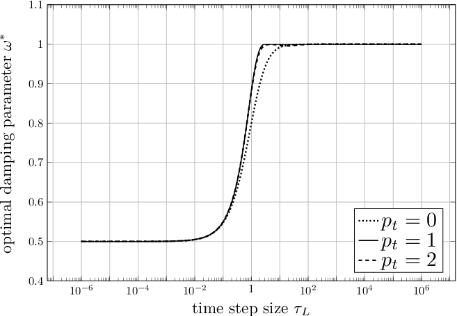
To show the convergence behavior of the damped block Jacobi smoother (10) with respect to the time step size $\tau_{L}$ , we now prove the following lemma for an arbitrary $\alpha\in\mathbb{R}$ .

Lemma 18.

For $\alpha\in\mathbb{R}$ and the optimal choice for the damping parameter

\displaystyle\omega_{t}^{\ast}=\begin{cases}\frac{1}{1+\alpha^{2}}&\alpha\geq 0,\\ 1&\alpha<0,\end{cases}

we have the estimate

\displaystyle\max_{\theta_{k}\in\Theta_{L}}\hat{S}(\omega_{t}^{\ast},\alpha,\theta_{k})\leq\frac{\left\lvert{\alpha}\right\rvert(1+\left\lvert{\alpha}\right\rvert)}{1+\alpha^{2}}.

Proof.

For the optimal damping parameter $\omega_{t}^{\ast}$ , we have

\left(\hat{S}(\omega_{t}^{\ast},\alpha,\theta_{k})\right)^{2}=\frac{\alpha^{2}}{1+\alpha^{2}}+\frac{2\alpha^{3}}{(1+\alpha^{2})^{2}}\cos(\theta_{k}).

For the case $\alpha\geq 0$ we therefore obtain

\displaystyle\argsup_{\theta_{k}\in[0,\pi]}\hat{S}(\omega_{t}^{\ast},\alpha,\theta_{k})=0.

Thus we have

\left(\hat{S}(\omega_{t}^{\ast},\alpha,0)\right)^{2}=\frac{\alpha^{2}+\alpha^{4}+2\alpha^{3}}{(1+\alpha^{2})^{2}}=\frac{\alpha^{2}(1+\alpha)^{2}}{(1+\alpha^{2})^{2}}.

For the case $\alpha<0$ we find that

\displaystyle\argsup_{\theta_{k}\in[0,\pi]}\hat{S}(\omega_{t}^{\ast},\alpha,\theta_{k})=\pi

and thus

\left(\hat{S}(\omega_{t}^{\ast},\alpha,0)\right)^{2}=\frac{\alpha^{2}+\alpha^{4}+2\left\lvert{\alpha}\right\rvert^{3}}{(1+\alpha^{2})^{2}}=\frac{\alpha^{2}(1+\left\lvert{\alpha}\right\rvert)^{2}}{(1+\alpha^{2})^{2}}.

The statement of this lemma follows with the fact that

\displaystyle\max_{\theta_{k}\in\Theta_{L}}\hat{S}(\omega_{t}^{\ast},\alpha,\theta_{k})\leq\sup_{\theta_{k}\in[0,\pi]}\hat{S}(\omega_{t}^{\ast},\alpha,\theta_{k}).

∎

Remark 19.

For sufficiently small values of $\alpha=\alpha(\tau_{L})$ , i.e. for sufficiently large time step sizes $\tau_{L}$ , it is shown in Lemma 18 that the convergence factor $\hat{S}(\omega_{t}^{\ast},\alpha(\tau_{L}),\theta_{k}^{\ast})$ of the block Jacobi smoother (10) is close to zero, see Figure 2a. Hence the block Jacobi smoother (10) is already a very good iterative solver.

All the estimates above are valid for arbitrary polynomial degrees $p_{t}\in\mathbb{N}_{0}$ . For the limiting case $p_{t}\rightarrow\infty$ , the function $\alpha(\tau_{L})$ is given by

\alpha(\tau_{L})=e^{-\tau_{L}},

since $\alpha(t)$ is the $(p_{t},p_{t}+1)$ subdiagonal Padé approximation of the exponential function $e^{-t}$ . Hence, the choice of the best damping parameter $\omega^{\ast}$ and the smoothing factors converge also to a limit function.

4.2 Two-grid analysis

We turn our attention now to the two-grid cycle for (8), for which the error satisfies

(18)

\displaystyle\bm{e}^{k+1}=\mathcal{M}_{\tau_{L}}\bm{e}^{k}:=\mathcal{S}_{\tau_{L}}^{\nu_{2}}\left[I-\mathcal{P}^{L}\mathcal{L}_{2\tau_{L}}^{-1}\mathcal{R}^{L}\mathcal{L}_{\tau_{L}}\right]\mathcal{S}_{\tau_{L}}^{\nu_{1}}\bm{e}^{k}.

We use again Fourier mode analysis, which would be exact for time periodic problems, see (13). We thus need to compute the Fourier symbol of the two-grid iteration matrix $\mathcal{M}_{\tau_{L}}$ . In Lemma 9 we already derived the local Fourier symbol for the system matrix $\tilde{\mathcal{L}}_{\tau_{L}}$ ,

\hat{\mathcal{L}}_{\tau_{L}}(\theta_{k}):=K_{\tau_{L}}+M_{\tau_{L}}-e^{-\mathbbm{i}\theta_{k}}N_{\tau_{L}}\in\mathbb{C}^{N_{t}\times N_{t}},

and the local Fourier symbol for the smoother $\tilde{\mathcal{S}}_{\tau_{L}}^{\nu}$ is given by

\hat{\mathcal{S}}_{\tau_{L}}^{\nu}(\theta_{k},\omega_{t}):=\left((1-\omega_{t})I_{N_{t}}+e^{-\mathbbm{i}\theta_{k}}\omega_{t}(K_{\tau_{L}}+M_{\tau_{L}})^{-1}N_{\tau_{L}}\right)^{\nu}\in\mathbb{C}^{N_{t}\times N_{t}},

see Lemma 10. For the local parts it is convenient to use the so called stencil notation: for the system matrix $\tilde{\mathcal{L}}_{\tau_{L}}$ , its stencil is

\displaystyle\widetilde{\mathcal{L}}_{\tau_{L}}:=\begin{bmatrix}-N_{\tau_{L}}&K_{\tau_{L}}+M_{\tau_{L}}&0\end{bmatrix},

and one smoothing iteration $\tilde{\mathcal{S}}_{\tau_{L}}^{\nu}$ , $\nu=1$ , is given in stencil notation by

\displaystyle\widetilde{\mathcal{S}}_{\tau_{L}}^{1}:=\begin{bmatrix}-\omega_{t}(K_{\tau_{L}}+M_{\tau_{L}})^{-1}N_{\tau_{L}}&(1-\omega_{t})I_{N_{t}}&0\end{bmatrix}.

Using periodic boundary conditions leads to the mapping properties

(19)

\displaystyle\tilde{\mathcal{L}}_{\tau_{L}}:\Psi_{L}(\theta_{k})\rightarrow\Psi_{L}(\theta_{k})\quad\text{and}\quad\tilde{\mathcal{S}}_{\tau_{L}}^{\nu}:\Psi_{L}(\theta_{k})\rightarrow\Psi_{L}(\theta_{k}).

We next analyze the mapping properties of the restriction and the prolongation operators, for which we need

Lemma 20.

The mapping $\gamma:\Theta_{L}^{\mathrm{low}}\rightarrow\Theta_{L}^{\mathrm{high}}$ with $\gamma(\theta_{k}):=\theta_{k}-\mathrm{sign}(\theta_{k})\pi$ is a one to one mapping.

Proof.

Let $\theta_{k}\in\Theta_{L}^{\mathrm{low}}$ . By definition we have

\theta_{k}=\frac{2k\pi}{N_{L}}\qquad\text{with}\quad k\in\left\{1-\frac{N_{L}}{4},\ldots,\frac{N_{L}}{4}\right\}.

For the mapping $\gamma$ we then obtain

\displaystyle\gamma(\theta_{k})=\theta_{k}-\mathrm{sign}(\theta_{k})\pi=\frac{2k\pi}{N_{L}}-\mathrm{sign}(\theta_{k})\pi=\frac{2(k-\mathrm{sign}(\theta_{k})\frac{N_{L}}{2})\pi}{N_{L}}=\frac{2\hat{k}\pi}{N_{L}},

with

\displaystyle\hat{k}=k-\mathrm{sign}(\theta_{k})\frac{N_{L}}{2}\in\left\{1-\frac{N_{L}}{2},\ldots,-\frac{N_{L}}{4}\right\}\cup\left\{\frac{N_{L}}{4}+1,\ldots,\frac{N_{L}}{2}\right\}.

This implies that $\gamma(\theta_{k})\in\Theta_{L}^{\mathrm{high}}$ and that $\mathrm{sign}(\gamma(\theta_{k}))=-\mathrm{sign}(\theta_{k})$ . Hence we have

\displaystyle\gamma(\gamma(\theta_{k}))=\gamma(\theta_{k})-\mathrm{sign}(\gamma(\theta_{k}))\pi=\gamma(\theta_{k})+\mathrm{sign}(\theta_{k})\pi=\theta_{k},

which completes the proof. ∎

Lemma 21.

The vector $\bm{u}=(\bm{u}_{1},\bm{u}_{2},\ldots,\bm{u}_{N_{L}})^{\top}\in\mathbb{R}^{N_{L}\,N_{t}}$ for $N_{L-1},N_{t}\in\mathbb{N}$ and $N_{L}=2N_{L-1}$ can be written as

\displaystyle\bm{u}=\sum_{\theta_{k}\in\theta_{L}^{\mathrm{low}}}\left[\bm{\psi}^{L}(\theta_{k})+\bm{\psi}^{L}(\gamma(\theta_{k}))\right],

where the vector $\bm{\psi}^{L}(\theta_{k})\in\mathbb{C}^{N_{t}N_{L}}$ is defined as in Lemma 6.

Proof.

Applying Lemma 6 and Lemma 20 proves the statement of this lemma with

	$\displaystyle\bm{u}$	$\displaystyle=\sum_{\theta_{k}\in\Theta_{L}}\bm{\psi}^{L}(\theta_{k})=\sum_{\theta_{k}\in\Theta_{L}^{\mathrm{low}}}\bm{\psi}^{L}(\theta_{k})+\sum_{\theta_{k}\in\Theta_{L}^{\mathrm{high}}}\bm{\psi}^{L}(\theta_{k})$
		$\displaystyle=\sum_{\theta_{k}\in\Theta_{L}^{\mathrm{low}}}\bm{\psi}^{L}(\theta_{k})+\sum_{\theta_{k}\in\Theta_{L}^{\mathrm{low}}}\bm{\psi}^{L}(\gamma(\theta_{k}))=\sum_{\theta_{k}\in\Theta_{L}^{\mathrm{low}}}\left[\bm{\psi}^{L}(\theta_{k})+\bm{\psi}^{L}(\gamma(\theta_{k}))\right].$

Lemma 21 motivates

Definition 22 (Space of harmonics).

For $N_{L},N_{t}\in\mathbb{N}$ and for a low frequency $\theta_{k}\in\Theta_{L}^{\mathrm{low}}$ let the vector $\bm{\Phi}^{L}(\theta_{k})\in\mathbb{C}^{N_{t}N_{L}}$ be defined as in Lemma 6. Then the linear space of harmonics with frequency $\theta_{k}$ is given by

	$\displaystyle\mathcal{E}_{L}(\theta_{k})$	$\displaystyle:=\mathrm{span}\left\{\bm{\Phi}^{L}(\theta_{k}),\bm{\Phi}^{L}(\gamma(\theta_{k}))\right\}$
		$\displaystyle\phantom{:}=\big\{\bm{\psi}^{L}(\theta_{k})\in\mathbb{C}^{N_{t}N_{L}}:\bm{\psi}_{n}^{L}(\theta_{k})=U_{1}\bm{\Phi}_{n}^{L}(\theta_{k})+U_{2}\bm{\Phi}_{n}^{L}(\gamma(\theta_{k})),$
		$\displaystyle\qquad\qquad\qquad\qquad\qquad\qquad n=1,\ldots,N_{L}\text{ and }U_{1},U_{2}\in\mathbb{C}^{N_{t}\times N_{t}}\big\}.$

Under the assumption of periodic boundary conditions, the mappings (19) imply the mapping properties

(20)

\displaystyle\tilde{\mathcal{L}}_{\tau_{L}}:\mathcal{E}_{L}(\theta_{k})\rightarrow\mathcal{E}_{L}(\theta_{k})\quad\text{and}\quad\tilde{\mathcal{S}}_{\tau_{L}}^{\nu}:\mathcal{E}_{L}(\theta_{k})\rightarrow\mathcal{E}_{L}(\theta_{k}),

with the mapping for the system matrix $\tilde{\mathcal{L}}_{\tau_{L}}$

(21)			$\displaystyle\begin{pmatrix}U_{1}\\ U_{2}\end{pmatrix}\mapsto\begin{pmatrix}\hat{\mathcal{L}}_{\tau_{L}}(\theta_{k})&0\\ 0&\hat{\mathcal{L}}_{\tau_{L}}(\gamma(\theta_{k}))\end{pmatrix}\begin{pmatrix}U_{1}\\ U_{2}\end{pmatrix},$
and the mapping for the smoother $\tilde{\mathcal{S}}_{\tau_{L}}^{\nu}$
(22)			$\displaystyle\begin{pmatrix}U_{1}\\ U_{2}\end{pmatrix}\mapsto\begin{pmatrix}\hat{\mathcal{S}}_{\tau_{L}}^{\nu}(\theta_{k},\omega_{t})&0\\ 0&\hat{\mathcal{S}}_{\tau_{L}}^{\nu}(\gamma(\theta_{k}),\omega_{t})\end{pmatrix}\begin{pmatrix}U_{1}\\ U_{2}\end{pmatrix}.$

We now analyze the two-grid cycle on the space of harmonics $\mathcal{E}_{L}(\theta_{k})$ for frequencies $\theta_{k}\in\Theta_{L}^{\mathrm{low}}$ . To do so, we further have to investigate the mapping properties of the restriction and prolongation operators $\mathcal{R}^{L}$ and $\mathcal{P}^{L}$ . The restriction operator is given by

(23)	$\displaystyle\mathcal{R}^{L}$	$\displaystyle:=\begin{pmatrix}R_{1}&R_{2}&&&&\\ &&R_{1}&R_{2}&&\\ &&&\ddots&\ddots&\\ &&&&R_{1}&R_{2}\end{pmatrix}\in\mathbb{R}^{N_{t}N_{L}\times N_{t}N_{L-1}},$
and the prolongation operator is given by
(24)	$\displaystyle\mathcal{P}^{L}$	$\displaystyle:=\begin{pmatrix}R_{1}^{\top}&&&\\ R_{2}^{\top}&&&\\ &R_{1}^{\top}&&\\ &R_{2}^{\top}&\ddots&\\ &&\ddots&R_{1}^{\top}\\ &&&R_{2}^{\top}\end{pmatrix}=(\mathcal{R}^{L})^{\top}\in\mathbb{R}^{N_{t}N_{L-1}\times N_{t}N_{L}},$

with the local prolongation matrices

\displaystyle R_{1}^{\top}:=M_{\tau_{L}}^{-1}\widetilde{M}_{\tau_{L}}^{1}\quad\text{and}\quad R_{2}^{\top}:=M_{\tau_{L}}^{-1}\widetilde{M}_{\tau_{L}}^{2},

where for basis functions $\left\{\psi_{k}\right\}_{k=1}^{N_{t}}\subset\mathbb{P}^{p_{t}}(0,\tau_{L})$ and $\left\{\widetilde{\psi}_{k}\right\}_{k=1}^{N_{t}}\subset\mathbb{P}^{p_{t}}(0,2\tau_{L})$ the local projection matrices from coarse to fine grids are defined for $k,\ell=1,\ldots,N_{t}$ by

\displaystyle\widetilde{M}_{\tau_{L}}^{1}[k,\ell]:=\int_{0}^{\tau_{L}}\widetilde{\psi}_{\ell}(t)\psi_{k}(t)\mathrm{d}t\quad\text{and}\quad\widetilde{M}_{\tau_{L}}^{2}[k,\ell]:=\int_{\tau_{L}}^{2\tau_{L}}\widetilde{\psi}_{\ell}(t)\psi_{k}(t+\tau)\mathrm{d}t.

To prove the mapping properties of the restriction operator $\mathcal{R}^{L}$ we need

Lemma 23.

Let $\bm{\psi}^{L}(\theta_{k})\in\Psi_{L}(\theta_{k})$ for $\theta_{k}\in\Theta_{L}$ . Then $\psi_{2n}^{L}(\theta_{k})=\psi_{n}^{L}(2\theta_{k})$ holds for $n=1,\ldots,N_{L-1}$ .

Proof.

Let $\bm{\psi}^{L}(\theta_{k})\in\Psi_{L}(\theta_{k})$ . Hence we have $\bm{\psi}_{n}^{L}(\theta_{k})=U\bm{\Phi}_{n}^{L}(\theta_{k})$ for $n=1,\dots,N_{L}$ . Then for $\bm{\Phi}_{2n}^{L}(\theta_{k})$ with $n\in\{1,\ldots,N_{L-1}\}$ we obtain for $\ell=1,\ldots,N_{t}$ that

\displaystyle\bm{\Phi}_{2n}^{L}(\theta_{k})[\ell]=\bm{\varphi}_{2n}(\theta_{k})=e^{\mathbbm{i}2n\theta_{k}}=\bm{\varphi}_{n}(2\theta_{k})=\bm{\Phi}_{n}^{L}(2\theta_{k})[\ell].

Hence the statement of this lemma follows from

\bm{\psi}_{2n}^{L}(\theta_{k})=U\bm{\Phi}_{2n}^{L}(\theta_{k})=U\bm{\Phi}_{n}^{L}(2\theta_{k})=\bm{\psi}_{n}^{L}(2\theta_{k}).

∎

The next two lemmas give the mapping properties of the restriction and extension:

Lemma 24.

Let $\theta_{k}\in\Theta_{L}^{\mathrm{low}}$ . Then the restriction operator $\mathcal{R}^{L}$ has the mapping property

\displaystyle\mathcal{R}^{L}:\mathcal{E}_{L}(\theta_{k})\rightarrow\Psi_{L-1}(2\theta_{k}),

with the mapping

\displaystyle\begin{pmatrix}U_{1}\\ U_{2}\end{pmatrix}\mapsto\begin{pmatrix}\hat{\mathcal{R}}(\theta_{k})&\hat{\mathcal{R}}(\gamma(\theta_{k}))\end{pmatrix}\begin{pmatrix}U_{1}\\ U_{2}\end{pmatrix}\in\mathbb{C}^{N_{t}\times N_{t}}

and the Fourier symbol

\displaystyle\hat{\mathcal{R}}(\theta_{k}):=e^{-\mathbbm{i}\theta_{k}}R_{1}+R_{2}.

Proof.

Let $\bm{\psi}^{L}(\theta_{k})\in\mathcal{E}_{L}(\theta_{k})$ for some frequency $\theta_{k}\in\Theta_{L}^{\mathrm{low}}$ with the linear combination $\bm{\psi}_{n}^{L}(\theta_{k})=U_{1}\bm{\Phi}_{n}^{L}(\theta_{k})+U_{2}\bm{\Phi}_{n}^{L}(\gamma(\theta_{k}))$ . Then for the Fourier mode $\bm{\Phi}^{L}(\theta_{\ell})$ with frequency $\theta_{\ell}\in\Theta_{L}$ we have for a fixed $n\in\{1,\ldots,N_{L-1}\}$

	$\displaystyle\left(\mathcal{R}^{L}\bm{\Phi}^{L}(\theta_{\ell})\right)_{n}$	$\displaystyle=R_{1}\bm{\Phi}_{2n-1}^{L}(\theta_{\ell})+R_{2}\bm{\Phi}_{2n}^{L}(\theta_{\ell})=\left[e^{-\mathbbm{i}\theta_{\ell}}R_{1}+R_{2}\right]\bm{\Phi}_{2n}^{L}(\theta_{\ell})$
		$\displaystyle=\left[e^{-\mathbbm{i}\theta_{\ell}}R_{1}+R_{2}\right]\bm{\Phi}_{n}^{L-1}(2\theta_{\ell}),$

since $\bm{\Phi}^{L}(\theta_{\ell})\in\Psi_{L}(\theta_{\ell})$ using Lemma 8, and also applying Lemma 23. Using this result for the vector $\bm{\psi}^{L}(\theta_{k})$ leads to

\displaystyle\left(\mathcal{R}^{L}\bm{\psi}^{L}(\theta_{k})\right)_{n}=\hat{\mathcal{R}}(\theta_{k})U_{1}\bm{\Phi}_{n}^{L-1}(2\theta_{k})+\hat{\mathcal{R}}(\gamma(\theta_{k}))U_{2}\bm{\Phi}_{n}^{L-1}(2\gamma(\theta_{k})).

For $i=1,\ldots,N_{t}$ we further have that

	$\displaystyle\bm{\Phi}_{n}^{L-1}(2\gamma(\theta_{k}))[i]$	$\displaystyle=\bm{\varphi}_{n}(2\gamma(\theta_{k}))=e^{\mathbbm{i}n2\gamma(\theta_{k})}=e^{\mathbbm{i}n2\theta_{k}-\mathbbm{i}\,\mathrm{sign}(\theta_{k})2\pi}$
		$\displaystyle=e^{\mathbbm{i}n2\theta_{k}}=\bm{\varphi}_{n}(2\theta_{k})=\bm{\Phi}_{n}^{L-1}(2\theta_{k})[i].$

Hence we obtain

\displaystyle\left(\mathcal{R}^{L}\bm{\psi}^{L}(\theta_{k})\right)_{n}=\left[\hat{\mathcal{R}}(\theta_{k})U_{1}+\hat{\mathcal{R}}(\gamma(\theta_{k}))U_{2}\right]\bm{\Phi}_{n}^{L-1}(2\theta_{k}),

which completes the proof. ∎

Lemma 25.

Let $\theta_{k}\in\Theta_{L}^{\mathrm{low}}$ . Then the the prolongation operator $\mathcal{P}^{L}$ has the mapping property

\displaystyle\mathcal{P}^{L}:\Psi_{L-1}(2\theta_{k})\rightarrow\mathcal{E}_{L}(\theta_{k}),

with the mapping

\displaystyle U\mapsto\begin{pmatrix}\hat{\mathcal{P}}(\theta_{k})\\ \hat{\mathcal{P}}(\gamma(\theta_{k}))\end{pmatrix}U\in\mathbb{C}^{2N_{t}\times N_{t}}

and the Fourier symbol

\displaystyle\hat{\mathcal{P}}(\theta_{k}):=\frac{1}{2}\left[e^{\mathbbm{i}\theta_{k}}R_{1}^{\top}+R_{2}^{\top}\right].

Proof.

For $\theta_{k}\in\Theta_{L}^{\mathrm{low}}$ let $\bm{\psi}^{L-1}(2\theta_{k})\in\Psi_{L-1}(2\theta_{k})$ with $\bm{\psi}_{\hat{n}}^{L-1}(2\theta_{k})=U\bm{\Phi}_{\hat{n}}^{L-1}(2\theta_{k})$ for $\hat{n}\in\left\{1,\ldots,N_{L-1}\right\}$ . We then define $\bm{\psi}^{L}(\theta_{k})\in\Psi_{L}(\theta_{k})$ as $\bm{\psi}_{n}^{L}(\theta_{k})=U\bm{\Phi}_{n}^{L}(\theta_{k})$ for $n\in\left\{1,\ldots,N_{L}\right\}$ and obtain

\displaystyle\left(\mathcal{P}^{L}\bm{\psi}^{L-1}(2\theta_{k})\right)_{2\hat{n}-1}=R_{1}^{\top}\bm{\psi}_{\hat{n}}^{L-1}(2\theta_{k})=R_{1}^{\top}\bm{\psi}_{2\hat{n}}^{L}(\theta_{k})=e^{\mathbbm{i}\theta_{k}}R_{1}^{\top}\bm{\psi}_{2\hat{n}-1}^{L}(\theta_{k}),

where we used Lemma 23 and Lemma 8. Similar computations also give

\displaystyle\left(\mathcal{P}^{L}\bm{\psi}^{L-1}(2\theta_{k})\right)_{2\hat{n}}

\displaystyle=R_{2}^{\top}\bm{\psi}_{\hat{n}}^{L-1}(2\theta_{k})=R_{2}^{\top}\bm{\psi}_{2\hat{n}}^{L}(\theta_{k}).

Hence we have for $n\in\left\{1,\ldots,N_{L}\right\}$

\displaystyle\left(\mathcal{P}^{L}\bm{\psi}^{L-1}(2\theta_{k})\right)_{n}=\begin{cases}e^{\mathbbm{i}\theta_{k}}R_{1}^{\top}\bm{\psi}_{n}^{L}(\theta_{k})&n\text{ odd},\\ R_{2}^{\top}\bm{\psi}_{n}^{L}(\theta_{k})&n\text{ even}\end{cases}\in\mathbb{C}^{N_{t}}.

For the image of the prolongation operator $\mathcal{P}^{L}$ to be contained in $\mathcal{E}_{L}(\theta_{k})$ , the following equations have to be satisfied for $n=1,\ldots,N_{L}$ :

(25)		$\displaystyle U_{1}\bm{\Phi}_{n}^{L}(\theta_{k})+U_{2}\bm{\Phi}_{n}^{L}(\gamma(\theta_{k}))$	$\displaystyle=e^{\mathbbm{i}\theta_{k}}R_{1}^{\top}U\bm{\Phi}_{n}^{L}(\theta_{k})$		$\displaystyle\text{for }n\text{ odd},$
(25)		$\displaystyle U_{1}\bm{\Phi}_{n}^{L}(\theta_{k})+U_{2}\bm{\Phi}_{n}^{L}(\gamma(\theta_{k}))$	$\displaystyle=R_{2}^{\top}U\bm{\Phi}_{n}^{L}(\theta_{k})$		$\displaystyle\text{for }n\text{ even}.$

Further computations show for $\ell=1,\ldots,N_{t}$ that

	$\displaystyle\bm{\Phi}_{n}^{L}(\gamma(\theta_{k}))[\ell]$	$\displaystyle=\bm{\varphi}_{n}(\gamma(\theta_{k}))=e^{\mathbbm{i}n\gamma(\theta_{k})}=e^{\mathbbm{i}n\theta_{k}-\mathbbm{i}\,\mathrm{sign}(\theta_{k})n\pi}=\bm{\varphi}_{n}(\theta_{k})e^{\mathbbm{i}\,\mathrm{sign}(\theta_{k})n\pi}$
		$\displaystyle=\bm{\Phi}_{n}^{L}(\theta_{k})[\ell]\begin{cases}1&n\text{ even},\\ -1&n\text{ odd}.\end{cases}$

Hence the equations (25) are equivalent to the system of linear equations

	$\displaystyle U_{1}-U_{2}$	$\displaystyle=e^{\mathbbm{i}\theta_{k}}R_{1}^{\top}U,$
	$\displaystyle U_{1}+U_{2}$	$\displaystyle=R_{2}^{\top}U.$

Solving for $U_{1}$ and $U_{2}$ results in

	$\displaystyle U_{1}$	$\displaystyle=\frac{1}{2}\left[e^{\mathbbm{i}\theta_{k}}R_{1}^{\top}+R_{2}^{\top}\right]=\hat{\mathcal{P}}(\theta_{k})U,$
	$\displaystyle U_{2}$	$\displaystyle=\frac{1}{2}\left[-e^{\mathbbm{i}\theta_{k}}R_{1}^{\top}+R_{2}^{\top}\right]=\frac{1}{2}\left[e^{\mathbbm{i}(\theta_{k}-\mathrm{sign}(\theta_{k})\pi)}R_{1}^{\top}+R_{2}^{\top}\right]$
		$\displaystyle=\frac{1}{2}\left[e^{\mathbbm{i}\gamma(\theta_{k})}R_{1}^{\top}+R_{2}^{\top}\right]=\hat{\mathcal{P}}(\gamma(\theta_{k}))U,$

which completes the proof. ∎

In view of Lemma 24 and Lemma 25, the stencil notations for the restriction and prolongation operators $\mathcal{R}^{L}$ and $\mathcal{P}^{L}$ are given by

\displaystyle\widetilde{\mathcal{R}}^{L}:=\begin{bmatrix}R_{1}&R_{2}&0\end{bmatrix}\quad\text{and}\quad\widetilde{\mathcal{P}}^{L}:=\frac{1}{2}\begin{bmatrix}0&R_{2}^{\top}&R_{1}^{\top}\end{bmatrix}.

For the two-grid operator $\mathcal{M}_{\tau_{L}}$ it now remains to prove the mapping property of the coarse grid operator $\tilde{\mathcal{L}}_{2\tau_{L}}^{-1}$ . Assuming periodic boundary conditions, we have for $\theta_{k}\in\Theta_{L-1}$ by using (19) that

\displaystyle\tilde{\mathcal{L}}_{2\tau_{L}}^{-1}:\Psi_{L-1}(\theta_{k})\rightarrow\Psi_{L-1}(\theta_{k}),

with the Fourier symbol

\displaystyle\hat{\mathcal{L}}_{2\tau_{L}}^{-1}(\theta_{k})=\left(K_{\tau_{L}}+M_{\tau_{L}}-e^{-\mathbbm{i}\theta_{k}}N_{\tau_{L}}\right)^{-1}=(\hat{\mathcal{L}}_{2\tau_{L}}(\theta_{k}))^{-1}\in\mathbb{C}^{N_{t}\times N_{t}}.

Lemma 26.

The frequency mapping

\beta:\Theta_{L}^{\mathrm{low}}\rightarrow\Theta_{L-1}\qquad\text{with}\qquad\theta_{k}\mapsto 2\theta_{k}

is a one to one mapping.

Proof.

For $\theta_{k}\in\Theta_{L}^{\mathrm{low}}$ we obtain

\displaystyle\beta(\theta_{k})=2\theta_{k}=2\frac{2k\pi}{N_{L}}=\frac{2k\pi}{\frac{N_{L}}{2}}=\frac{2k\pi}{N_{L-1}}\in\Theta_{L-1}.

The proof of this lemma then follows from the identity

\displaystyle k\in\left\{1-\frac{N_{L}}{4},\ldots,\frac{N_{L}}{4}\right\}=\left\{1-\frac{N_{L-1}}{2},\ldots,\frac{N_{L-1}}{2}\right\}.

∎

With Lemma 26 we now have for $\theta_{k}\in\Theta_{L}^{\mathrm{low}}$ the coarse grid operator mapping property

(26)

\displaystyle\tilde{\mathcal{L}}_{2\tau_{L}}^{-1}:\Psi_{L-1}(2\theta_{k})\rightarrow\Psi_{L-1}(2\theta_{k}).

We are now able to prove the following theorem for the two-grid operator $\mathcal{M}_{\tau_{L}}$ .

Theorem 27.

Let $\theta_{k}\in\Theta_{L}^{\mathrm{low}}$ . With time periodic boundary conditions, the two-grid operator $\mathcal{M}_{\tau_{L}}$ has the mapping property

\displaystyle\mathcal{M}_{\tau_{L}}:\mathcal{E}_{L}(\theta_{k})\rightarrow\mathcal{E}_{L}(\theta_{k}),

with the mapping

\displaystyle\begin{pmatrix}U_{1}\\ U_{2}\end{pmatrix}\mapsto\hat{\mathcal{M}}(\theta_{k})\begin{pmatrix}U_{1}\\ U_{2}\end{pmatrix}

and the iteration matrix

\displaystyle\hat{\mathcal{M}}(\theta_{k}):=\begin{pmatrix}\hat{\mathcal{S}}_{\tau_{L}}^{\nu_{2}}(\theta_{k},\omega_{t})&0\\ 0&\hat{\mathcal{S}}_{\tau_{L}}^{\nu_{2}}(\gamma(\theta_{k}),\omega_{t})\end{pmatrix}\mathcal{K}(\theta_{k})\begin{pmatrix}\hat{\mathcal{S}}_{\tau_{L}}^{\nu_{1}}(\theta_{k},\omega_{t})&0\\ 0&\hat{\mathcal{S}}_{\tau_{L}}^{\nu_{1}}(\gamma(\theta_{k}),\omega_{t})\end{pmatrix}

with

\displaystyle\mathcal{K}(\theta_{k}):=I_{2N_{t}}-\begin{pmatrix}\hat{\mathcal{P}}(\theta_{k})\\ \hat{\mathcal{P}}(\gamma(\theta_{k}))\end{pmatrix}(\hat{\mathcal{L}}_{2\tau_{L}}(2\theta_{k}))^{-1}\begin{pmatrix}\hat{\mathcal{R}}(\theta_{k})^{\top}\\ \hat{\mathcal{R}}(\gamma(\theta_{k}))^{\top}\end{pmatrix}^{\top}\begin{pmatrix}\hat{\mathcal{L}}_{\tau_{L}}(\theta_{k})&0\\ 0&\hat{\mathcal{L}}_{\tau_{L}}(\gamma(\theta_{k}))\end{pmatrix}.

Proof.

The statement of this theorem is a direct consequence of Lemma 24, Lemma 25 and the mapping properties (20) and (26). ∎

We now write the initial error $\bm{e}^{0}=\bm{u}-\bm{u}^{0}$ as

\bm{e}^{0}=\sum_{\theta_{k}\in\Theta_{L}^{\mathrm{low}}}\left[\bm{\psi}^{L}(\theta_{k})+\bm{\psi}^{L}(\gamma(\theta_{k}))\right],

with $\bm{\psi}^{L}(\theta_{k})+\bm{\psi}^{L}(\gamma(\theta_{k}))\in\mathcal{E}_{L}(\theta_{k})$ for all $\theta_{k}\in\Theta_{L}^{\mathrm{low}}$ , see Lemma 21. In view of Theorem 27 we can analyze the asymptotic behavior of the two-grid cycle by simply computing the largest spectral radius of $\hat{\mathcal{M}}(\theta_{k})\in\mathbb{C}^{2N_{t}\times 2N_{t}}$ with respect to the low frequencies $\theta_{k}\in\Theta_{L}^{\mathrm{low}}$ . This motivates

Definition 28 (Asymptotic two-grid convergence factor).

For the two-grid iteration matrix $\mathcal{M}_{\tau_{L}}$ , we define the asymptotic convergence factor

\displaystyle\varrho(\mathcal{M}_{\tau_{L}}):=\max\left\{\varrho\left(\hat{\mathcal{M}}(\theta_{k})\right):\theta_{k}\in\Theta_{L}^{\mathrm{low}}\right\}.

For the simplest case, i.e. for the polynomial degree $p_{t}=0$ , we have to compute the spectral radius of the $2\times 2$ iteration matrix $\hat{\mathcal{M}}(\theta_{k})$ . Using one pre and post smoothing step, i.e. $\nu_{1}=\nu_{2}=1$ , we find that the spectral radius of $\hat{\mathcal{M}}(\theta_{k})\in\mathbb{C}^{2\times 2}$ is

\displaystyle\varrho\left(\hat{\mathcal{M}}(\theta_{k})\right)=\left\lvert{\frac{4(1+\tau_{L})^{2}\left(\sin(\theta_{k})\right)^{2}+\tau_{L}^{2}(1+2\tau_{L}-e^{2\mathbbm{i}\theta_{k}})}{(2+\tau_{L}(2+\tau_{L}))^{2}\left((1+2\tau_{L})e^{2\mathbbm{i}\theta_{k}}-1\right)}}\right\rvert.

Further calculations show that the maximum of $\varrho\left(\hat{\mathcal{M}}(\theta_{k})\right)$ with respect to the low frequencies $\theta_{k}\in\Theta_{L}^{\mathrm{low}}$ is obtained for $\theta_{k}^{\ast}=\frac{\pi}{2}$ . Hence for this simple case we can compute the asymptotic convergence factor explicitly,

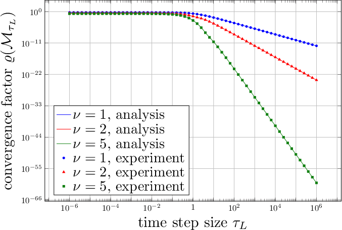
\displaystyle\varrho(\mathcal{M}_{\tau_{L}})=\frac{1}{2+2\tau_{l}+\tau_{L}^{2}}\in[0,\frac{1}{2}]\qquad\text{for all }\tau_{L}\geq 0.

For periodic boundary conditions we therefore conclude that the two-grid cycle converges for any $\tau_{L}\geq 0$ to the exact solution, since $\varrho(\mathcal{M}_{\tau_{L}})\leq\frac{1}{2}$ for all $\tau_{L}\geq 0$ . Furthermore, we obtain that the asymptotic convergence factor $\varrho(\mathcal{M}_{\tau_{L}})$ gets very small for large time step sizes, i.e. $\varrho(\mathcal{M}_{\tau_{L}})=\mathcal{O}(\tau_{L}^{-2})$ . This results from the fact that the smoother itself is already an efficient iterative solver for large time step sizes, see Remark 19.

For higher polynomial degrees $p_{t}$ , we have to compute the eigenvalues of the $2(p_{t}+1)\times 2(p_{t}+1)$ iteration matrix $\hat{\mathcal{M}}(\theta_{k})$ , which are difficult to obtain in closed form. We thus compute numerically for all frequencies $\theta_{k}\in\Theta_{L}^{\mathrm{low}}$ the eigenvalues of $\hat{\mathcal{M}}(\theta_{k})$ to determine the asymptotic convergence factor $\varrho\left(\hat{\mathcal{M}}(\theta_{k})\right)$ for a given time step size $\tau_{L}$ .

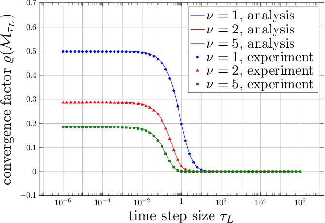
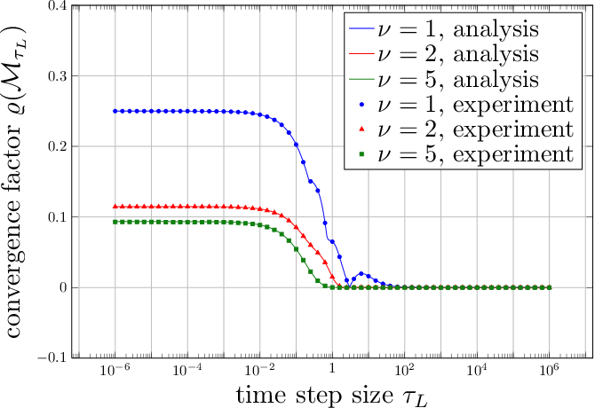
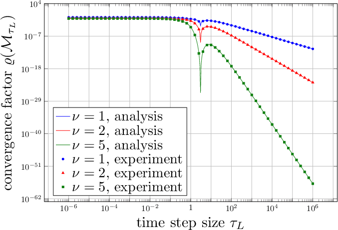
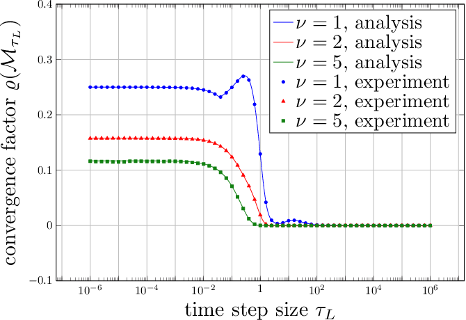
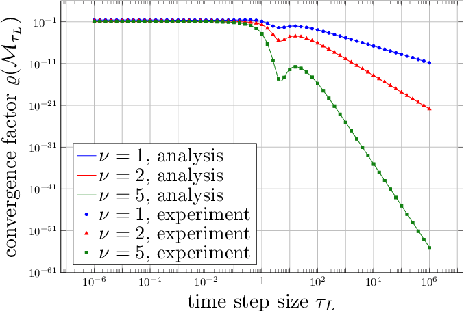
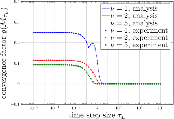
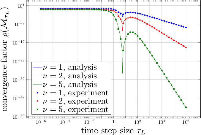
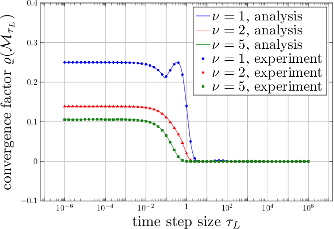
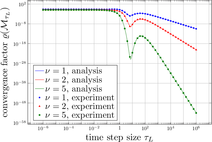
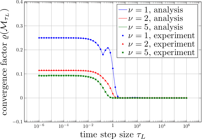
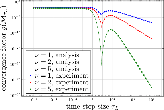
We show in Figures 3–8 the theoretical asymptotic convergence factors $\varrho\left(\hat{\mathcal{M}}(\theta_{k})\right)$ as solid lines for $\tau_{L}\in[10^{-6},10^{6}]$ and $p_{t}\in\{0,1,\ldots,5\}$ and three numbers of smoothing iterations $\nu_{1}=\nu_{2}=\nu$ with $\nu\in\{1,2,5\}$ . We see that for higher polynomial degrees $p_{t}\geq 1$ the theoretical convergence factors are about half the theoretical convergence factor of the lowest order case $p_{t}=0$ . We also notice that the theoretical convergence factors are close to zero for large time step sizes $\tau_{L}$ , as expected, see Remark 19. Furthermore, for odd polynomial degrees $p_{t}$ we observe a peak in the plots for the theoretical convergence factors. This is because for odd polynomial degrees, the $(p_{t},p_{t}+1)$ subdiagonal Padé approximation of $e^{-t}$ has exactly one zero for $t>0$ . Hence for one $\tau_{L}^{\ast}>0$ we have $\alpha(\tau_{L}^{\ast})=0$ which implies for the smoothing factor $\mu_{S}=0$ , see Lemma 18. Hence the application of only two smoothing iterations results in an exact solver.

We also show in the same Figures 3–8, using dots, triangles and squares, the numerically computed convergence factors when solving the equation

\mathcal{L}_{\tau_{L}}\bm{u}=\bm{f}

with our two-grid cycle. We use $N_{L}=1024$ time steps with a zero right hand side, i.e. $\bm{f}=\mathbf{0}$ , and a random initial vector $\bm{u}^{0}$ with values between zero and one. The numerical convergence factor we measure is

\displaystyle\max_{k=1,\ldots,N_{\mathrm{iter}}}\frac{{\left\lVert{\bm{r}^{k+1}}\right\rVert}_{2}}{{\left\lVert{\bm{r}^{k}}\right\rVert}_{2}},\quad\text{with }\bm{r}^{k}:=\bm{f}-\mathcal{L}_{\tau_{L}}\bm{u}^{k},

where $N_{\mathrm{iter}}\in\mathbb{N}$ , $N_{\mathrm{iter}}\leq 250$ is the number of two-grid iterations used until we have reached a given relative error reduction of $\varepsilon_{\mathrm{MG}}$ . To measure the asymptotic behavior of the two-grid cycle, we have to use quite a small tolerance $\varepsilon_{\mathrm{MG}}=10^{-140}$ , since in the pre-asymptotic range the convergence rates of the two-grid cycle are in fact even better than our asymptotic estimate. We see that the theoretical results from the Fourier mode analysis agree very well with the numerical results, even though the Fourier mode analysis is only rigorous for time periodic conditions.

5 Numerical example

In this example we test the weak and strong scaling behavior of our new time multigrid algorithm. We use different polynomial degrees $p_{t}\in\{0,1,5,10,20\}$ and a fixed time step size $\tau=10^{-6}$ . For a random initial guess and a zero right hand side we run the algorithm until we have reached a relative error reduction of $\varepsilon_{\mathrm{MG}}=10^{-8}$ . We first study the weak scaling behavior by using a fixed number of time steps per core ( $32\;768$ ), and we increase the number of cores when increasing the number of time steps. In Table 1a, we give computation times for different numbers of cores and polynomial degrees. We observe excellent weak scaling, i.e. the computation times remain bounded when we increase the number of cores. We next study the strong scaling behavior by fixing the problem size, i.e. we use $1\;048\;576$ time steps in this example. Then we increase the number of cores from $1$ up to $32\;768$ . In Table 1b the computation times are given for different number of cores and polynomial degrees. We observe that the computation costs are basically divided by a factor of two if we double the number of cores, only for $32\;768$ cores and $p_{t}\in\{0,1,5\}$ we obtain no speedup any more, since the local problems are to small, i.e. for $p_{t}=0$ one core has to solve for only $32$ unknowns.

These computations were performed on the Monte Rosa supercomputer at the Swiss National Supercomputing Centre CSCS in Lugano.

cores	time steps	$p_{t}=0$	$p_{t}=1$	$p_{t}=5$	$p_{t}=10$	$p_{t}=20$
$1$	$32\;768$	$3.96$	$2.45$	$3.60$	$7.97$	$17.77$
$2$	$65\;536$	$5.30$	$3.39$	$5.10$	$10.74$	$25.83$
$4$	$131\;072$	$5.34$	$3.38$	$5.45$	$10.84$	$26.13$
$8$	$262\;144$	$5.95$	$3.77$	$5.75$	$11.70$	$28.54$
$16$	$524\;288$	$5.94$	$3.77$	$5.78$	$11.69$	$28.61$
$32$	$1\;048\;576$	$5.96$	$3.80$	$5.87$	$11.73$	$27.21$
$64$	$2\;097\;152$	$7.92$	$4.73$	$6.68$	$12.62$	$27.96$
$128$	$4\;194\;304$	$8.03$	$4.74$	$6.66$	$12.76$	$28.52$
$256$	$8\;388\;608$	$8.09$	$4.91$	$6.80$	$12.90$	$28.29$
$512$	$16\;777\;216$	$8.06$	$4.79$	$6.75$	$12.82$	$29.13$
$1\;024$	$33\;554\;432$	$7.96$	$4.75$	$6.69$	$13.01$	$28.89$
$2\;048$	$67\;108\;864$	$8.06$	$4.79$	$6.73$	$13.02$	$28.86$
$4\;096$	$134\;217\;728$	$8.14$	$4.80$	$6.77$	$12.77$	$29.18$
$8\;192$	$268\;435\;456$	$8.14$	$4.89$	$6.84$	$13.03$	$29.23$
$16\;384$	$536\;870\;912$	$8.10$	$4.80$	$6.82$	$13.25$	$29.52$
$32\;768$	$1\;073\;741\;824$	$8.21$	$4.94$	$6.90$	$13.19$	$29.03$

(a) Weak scaling results.

cores	time steps	$p_{t}=0$	$p_{t}=1$	$p_{t}=5$	$p_{t}=10$	$p_{t}=20$
$1$	$1\;048\;576$	$129.11$	$78.79$	$117.99$	$254.95$	$535.43$
$2$	$1\;048\;576$	$85.66$	$54.69$	$82.36$	$172.46$	$396.71$
$4$	$1\;048\;576$	$42.90$	$27.22$	$41.17$	$86.81$	$199.71$
$8$	$1\;048\;576$	$23.83$	$15.08$	$22.90$	$46.87$	$107.77$
$16$	$1\;048\;576$	$11.91$	$7.57$	$11.50$	$23.40$	$54.06$
$32$	$1\;048\;576$	$5.96$	$3.80$	$5.87$	$11.73$	$27.21$
$64$	$1\;048\;576$	$3.98$	$2.45$	$3.31$	$6.50$	$13.70$
$128$	$1\;048\;576$	$1.97$	$1.18$	$1.67$	$3.23$	$6.97$
$256$	$1\;048\;576$	$0.984$	$0.598$	$0.808$	$1.57$	$3.49$
$512$	$1\;048\;576$	$0.508$	$0.299$	$0.407$	$0.787$	$1.77$
$1\;024$	$1\;048\;576$	$0.264$	$0.155$	$0.210$	$0.444$	$0.904$
$2\;048$	$1\;048\;576$	$0.146$	$0.0864$	$0.114$	$0.210$	$0.465$
$4\;096$	$1\;048\;576$	$0.0861$	$0.0506$	$0.0653$	$0.116$	$0.243$
$8\;192$	$1\;048\;576$	$0.0548$	$0.0329$	$0.0405$	$0.0743$	$0.129$
$16\;384$	$1\;048\;576$	$0.0400$	$0.0230$	$0.0272$	$0.0424$	$0.0767$
$32\;768$	$1\;048\;576$	$0.0511$	$0.0241$	$0.0288$	$0.0376$	$0.0608$

(b) Strong scaling results.

Table 1: Scaling results with solving times in seconds.

6 Conclusions

We focused in this paper on the analysis of the multigrid method in time, and our model problem did not contain an operator in space. To fully leverage the speedup, we consider now the time dependent heat equation $\partial_{t}u=\Delta u+f$ . Applying our time multigrid algorithm requires now in each step of the block Jacobi smoother the solution of Laplace like problems, which we do by just applying one V-cycle of spatial multi-grid. Doing so, we obtain a space-time parallel method which takes on one processor for a problem of size $131\;120\;896$ a solution time of $10416.90$ seconds, which is about the same as for forward substitution which took $9970.89$ seconds, but which can run in parallel on 2048 cores in about $10$ seconds, about one thousand times faster than using forward substitution. These results have been computed on the Vienna Scientific Cluster VSC-2. The precise analysis of this space-time multigrid algorithm builds on the results we presented in this paper, but requires techniques for the spatial part that will appear elsewhere.

Acknowledgments

We thank Ernst Hairer for his help with Theorem 1, and Rolf Krause and Daniel Ruprecht for the simulations we were allowed to perform on the Monte Rosa supercomputer in Manno.

References

[1] A. Brandt. Multi-level adaptive solutions to boundary-value problems. Math. Comp., 31:333–390, 1977.
[2] A. Brandt. Rigorous quantitative analysis of multigrid. I. Constant coefficients two-level cycle with ${L}_{2}$ -norm. SIAM J. Numer. Anal., 31:1695–1730, 1994.
[3] F. Chipman. A-stable Runge-Kutta processes. Nordisk Tidskr. Informationsbehandling (BIT), 11:384–388, 1971.
[4] M. Delfour, W. Hager, and F. Trochu. Discontinuous Galerkin methods for ordinary differential equations. Math. Comp., 36:455–473, 1981.
[5] B. Ehle. On Padé approximations to the exponential function and A-stable methods for the numerical solution of initial value problems. PhD thesis, Technical Report CSRR 2010, Dept. AACS Univ. of Waterloo Ontario Canada, 1969.
[6] M. Emmett and M. L. Minion. Toward an efficient parallel in time method for partial differential equations. Comm. App. Math. and Comp. Sci, 7(1):105–132, 2012.
[7] R. Falgout, S. Friedhoff, T. Kolev, S. MacLachlan, , and J. Schröder. Parallel time integration with multigrid. submitted, 2014.
[8] M. J. Gander. 50 years of time parallel time integration. In Multiple Shooting and Time Domain Decomposition Methods. Springer Verlag, 2014.
[9] M. J. Gander and S. Güttel. ParaExp: A parallel integrator for linear initial-value problems. SIAM Journal on Scientific Computing, 35(2):C123–C142, 2013.
[10] M. J. Gander and E. Hairer. Nonlinear convergence analysis for the parareal algorithm. In O. B. Widlund and D. E. Keyes, editors, Domain Decomposition Methods in Science and Engineering XVII, volume 60 of Lecture Notes in Computational Science and Engineering, pages 45–56. Springer, 2008.
[11] M. J. Gander and L. Halpern. Optimized Schwarz waveform relaxation methods for advection reaction diffusion problems. SIAM J. Numer. Anal., 45(2):666–697, 2007.
[12] M. J. Gander and L. Halpern. A direct solver for time parallelization. In 22nd international Conference of Domain Decomposition Methods. Springer, 2014.
[13] M. J. Gander, L. Halpern, and F. Nataf. Optimal Schwarz waveform relaxation for the one dimensional wave equation. SIAM Journal of Numerical Analysis, 41(5):1643–1681, 2003.
[14] M. J. Gander and A. M. Stuart. Space-time continuous analysis of waveform relaxation for the heat equation. SIAM J. Sci. Comput., 19(6):2014–2031, 1998.
[15] M. J. Gander and S. Vandewalle. Analysis of the parareal time-parallel time-integration method. SIAM Journal on Scientific Computing, 29(2):556–578, 2007.
[16] W. Hackbusch. Parabolic multi-grid methods. In R. Glowinski and J.-L. Lions, editors, Computing Methods in Applied Sciences and Engineering, VI, pages 189–197. North-Holland, 1984.
[17] E. Hairer, C. Lubich, and G. Wanner. Geometric numerical integration. Structure-preserving algorithms for ordinary differential equations. Springer Series in Computational Mathematics, 31. Springer, Heidelberg, 2010.
[18] E. Hairer and G. Wanner. Solving ordinary differential equations. II. Stiff and differential-algebraic problems. Springer Series in Computational Mathematics, 14. Springer-Verlag, Berlin, 2010.
[19] G. Horton and S. Vandewalle. A space-time multigrid method for parabolic partial differential equations. SIAM Journal on Scientific Computing, 16(4):848–864, 1995.
[20] P. Lasaint and P.-A. Raviart. On a finite element method for solving the neutron transport equation. Mathematical aspects of finite elements in partial differential equations (Proc. Sympos., Math. Res. Center, Univ. Wisconsin, Madison, Wis., 1974), pages 89–123. Publication No. 33, Math. Res. Center, Univ. of Wisconsin–Madison, Academic Press, New York, 1974.
[21] J.-L. Lions, Y. Maday, and G. Turinici. A ”parareal” in time discretization of PDE’s. C. R. Acad. Sci. Paris Sér. I Math., 332:661–668, 2001.
[22] C. Lubich and A. Ostermann. Multi-grid dynamic iteration for parabolic equations. BIT, 27(2):216–234, 1987.
[23] Y. Maday and E. M. Rønquist. Parallelization in time through tensor-product space–time solvers. Comptes Rendus Mathematique, 346(1):113–118, 2008.
[24] M. Neumüller. Space-Time Methods: Fast Solvers and Applications. PhD thesis, University of Graz, 2013.
[25] W. Reed and T. Hill. Triangular mesh methods for the neutron transport equation. Tech Report LAUR73479 Los Alamos National Laboratory, Technical, Issue: LA-UR-73-479:1–23, 1973.
[26] R. Speck, D. Ruprecht, M. Emmett, M. Minion, M. Bolten, and R. Krause. A multi-level spectral deferred correction method. arXiv preprint arXiv:1307.1312, 2013.
[27] R. Speck, D. Ruprecht, R. Krause, M. Emmett, M. Minion, M. Winkel, and P. Gibbon. A massively space-time parallel n-body solver. In Proceedings of the International Conference on High Performance Computing, Networking, Storage and Analysis, page 92. IEEE Computer Society Press, 2012.
[28] K. Stüben and U. Trottenberg. Multigrid methods: fundamental algorithms, model problem analysis and applications. GMD-Studien [GMD Studies], 96. Gesellschaft für Mathematik und Datenverarbeitung mbH, St. Augustin, 1985.
[29] U. Trottenberg, C. W. Oosterlee, and A. Schüller. Multigrid. Academic Press, Inc., San Diego, 2001.
[30] P. Wesseling. An Introduction to Multigrid Methods. John Wiley & Sons Ltd., 1992. Corrected Reprint. Philadelphia: R.T. Edwards, Inc., 2004.