Subspace Alignment For Domain Adaptation
Abstract
In this paper, we introduce a new domain adaptation (DA) algorithm where the source and target domains are represented by subspaces spanned by eigenvectors. Our method seeks a domain invariant feature space by learning a mapping function which aligns the source subspace with the target one. We show that the solution of the corresponding optimization problem can be obtained in a simple closed form, leading to an extremely fast algorithm. We present two approaches to determine the only hyper-parameter in our method corresponding to the size of the subspaces. In the first approach we tune the size of subspaces using a theoretical bound on the stability of the obtained result. In the second approach, we use maximum likelihood estimation to determine the subspace size, which is particularly useful for high dimensional data. Apart from PCA, we propose a subspace creation method that outperform partial least squares (PLS) and linear discriminant analysis (LDA) in domain adaptation. We test our method on various datasets and show that, despite its intrinsic simplicity, it outperforms state of the art DA methods.
1 Introduction
In classification, it is typically assumed that the test data comes from the same distribution as that of the labeled training data. However, many real world applications, especially in computer vision, challenge this assumption (see, e.g., the study on dataset bias in [26]). In this context, the learner must take special care during the learning process to infer models that adapt well to the test data they are deployed on. For example, images collected from a DSLR camera are different from those taken with a web camera. A classifier that is trained on the former would likely fail to classify the latter correctly if applied without adaptation. Likewise, in face recognition the objective is to identify a person using available training images. However, the test images may arise from very different capturing conditions than the ones in the training set. In image annotation, the training images (such as ImageNet) could be very different from the images that we need to annotate (for example key frames extracted from an old video). These are some examples where training and test data are drawn from different distributions.

We refer to these different but related joint distributions as domains. Formally, if we denote as the data distribution and the label distribution of domain , then the source domain and the target domain have different joint distributions . In order to build robust classifiers, it is thus necessary to take into account the shift between these two distributions. Methods that are designed to overcome this shift in domains are known as domain adaptation (DA) methods. DA typically aims at making use of information coming from both source and target domains during the learning process to adapt automatically. One usually differentiates between two scenarios: (1) the unsupervised setting where the training consists of labeled source data and unlabeled target examples (see [19] for a survey); and (2) the semi-supervised case where a large number of labels are available for the source domain and only a few labels are provided for the target domain. In this paper, we focus on the most difficult, unsupervised scenario.
As illustrated by recent results [12, 13], subspace based domain adaptation seems to be a promising approach to tackle unsupervised visual DA problems. In [13], Gopalan et al. generate intermediate representations in the form of subspaces along the geodesic path connecting the source subspace and the target subspace on the Grassmann manifold. Then, the source data are projected onto these subspaces and a classifier is learned. In [12], Gong et al. propose a geodesic flow kernel which models incremental changes between the source and target domains. In both papers, a set of intermediate subspaces are used to model the shift between the two domains.
In this paper, we also make use of subspaces, one for each domain. We construct a subspace of size , e.g. composed of the d most important eigenvectors induced by principle component analysis (PCA). However, we do not construct a set of intermediate subspaces. Following the theoretical recommendations of Ben-David et al. [3], we suggest to directly reduce the discrepancy between the two domains by moving the source and target subspaces closer. This is achieved by optimizing a mapping function that transforms the source subspace into the target one. Based on this simple idea, we design a new DA approach called subspace alignment. The idea behind our method is illustrated in Figure 1. The source domain is represented by the source subspace and the target domain by target subspace . Then we align/transform the source subspace using matrix such that the aligned source subspace is as close as possible to the target subspace in the Bregman divergence perspective. Then we project source data to the target aligned source subspace () and the target data to the target subspace and learn a classifier on subspace. We use this classifier to classify data in the target subspace. The advantage of our method is two-fold: (1) by adapting the bases of the subspaces, our approach is global as it manipulates the global co-variance matrices. This allows us to induce robust classifiers not subject to local perturbations (in contrast to metric learning-based domain adaptation approaches that need to consider pairwise or triplet-based constraints for inducing the metric) and (2) by aligning the source and target subspaces, our method is intrinsically regularized: we do not need to tune regularization parameters in the objective as imposed by a lot of optimization-based DA methods.
Our subspace alignment is achieved by optimizing a mapping function which takes the form of a transformation matrix . We show that the optimal solution corresponds in fact to the covariance matrix between the source and target eigenvectors. From this transformation matrix, we derive a similarity function to compare a source data with a target example . Thanks to a consistency theorem, we prove that , which captures the idiosyncrasies of the training data, converges uniformly to its expected value. We show that we can make use of this theoretical result to tune the hyper-parameter (the dimensionality of the subspaces). This tends to make our method parameter-free. The similarity function can be used directly in a nearest neighbour classifier. Alternatively, we can also learn a global classifier such as a support vector machine on the source data after mapping them onto the target aligned source subspace.
As suggested by Ben David et al. [3], a reduction of the divergence between the two domains is required to adapt well. In other words, the ability of a DA algorithm to actually reduce that discrepancy is a good indication of its performance. A usual way to estimate the divergence consists in learning a linear classifier to discriminate between source and target instances, respectively pseudo-labeled with 0 and 1. In this context, the higher the error of , the smaller the divergence. While such a strategy gives us some insight about the ability for a global learning algorithm (e.g. SVM) to be efficient on both domains, it does not seem to be suited to deal with local classifiers, such as the -nearest neighbors. To overcome this limitation, we introduce a new empirical divergence specifically dedicated to local classifiers. We show through our experimental results that our DA method allows us to drastically reduce both empirical divergences.
This paper is an extended version of our previous work [11]. We address a few limitations of the previous subspace alignment (SA) based DA method. First, the work in [11] does not use source label information during the subspace creation. Methods such as partial least squares (PLS) or linear discriminant analysis (LDA) seem relevant for this task. However, applying different subspace creation methods such as PLS/LDA only for the source domain and PCA for the target domain may cause additional discrepancies between the source and the target domains. Moreover, LDA has a maximum dimensionality equal to the number of classes. To overcome these limitations, we use an existing metric learning algorithm (ITML [9]) to create subspaces in a supervised manner, then use PCA on both the source and the target domain. Even though ITML has been used before for domain adaptation (e.g. [24]), to the best of our knowledge, it has never been used to create linear subspaces in conjunction with PCA to improve subspace-based domain adaptation methods. We also introduce a novel large margin subspace alignment (LMSA) method where the objective is to learn the domain adaptive matrix while exploiting the source label information to obtain a discriminative solution. We experimentally show that both these methods are useful in practice.
Secondly, the cross-validation procedure presented in [11] to estimate the subspace dimensionality could be computationally expensive for high dimensional data as discussed in recent reviews [22]. We propose a fast and well founded approach to estimate the subspace dimensionality and reduce computational complexity of our SA method. We call this new extension of SA method as SA-MLE. We show promising results using high dimensional data such as Fisher vectors using SA-MLE method. Thirdly, we present a mutual information based perspective of our SA method. We show that after the adaptation, with SA method we can increase the mutual information between the source and the target domains. We also include further analysis and comparisons in the experimental section. We provide a detailed analysis of our DA method over several features such as bag-of-words, Fisher vectors [23] and DECAF [10] features. We also analyze how subspace-based DA methods perform over different dictionary sizes and feature normalization methods such as z-normalization.
The rest of the paper is organized as follows. We present the related work in section 2. Section 3 is devoted to the presentation of our domain adaptation method and the consistency theorem on the similarity measure deduced from the learned mapping function. We also present our supervised PCA method and the SA-MLE method in section 3. In section 4, a comparative study is performed on various datasets. We conclude in section 5.
2 Related work
DA has been widely studied in the literature and is of great importance in many areas such as natural language processing [6] and computer vision [26]. In this paper, we focus on the unsupervised domain adaptation setting that is well suited to vision problems since it does not require any labeling information from the target domain. This setting makes the problem very challenging. An important issue is to find out the relationship between the two domains. A classical trend is to assume the existence of a domain invariant feature space and the objective of a large range of DA work is to approximate this space [19].
A classical strategy related to our work consists of learning a new domain-invariant feature representation by looking for a new projection space. PCA based DA methods have then been naturally investigated [8, 20, 21, 1] in order to find a common latent space where the difference between the marginal distributions of the two domains is minimized with respect to the Maximum Mean Discrepancy (MMD) divergence. Very recently, Shao et al. [25] have presented a very similar approach to ours. In this work Shao et al. present a low-rank transfer subspace learning technique that exploits the locality aware reconstruction in a similar way to manifold learning.
Other strategies have been explored as well such as using metric learning approaches [16, 24] or canonical correlation analysis methods over different views of the data to find a coupled source-target subspace [5] where one assumes the existence of a performing linear classifier on the two domains.
In the structural correspondence learning method of [6], Blitzer et al. propose to create a new feature space by identifying correspondences among features from different domains by modeling their correlations with pivot features. Then, they concatenate source and target data using this feature representation and apply PCA to find a relevant common projection. In [7], Chang transforms the source data into an intermediate representation such that each transformed source sample can be linearly reconstructed by the target samples. This is however a local approach. Local methods may fail to capture the global distribution information of the source,target domains. Moreover it is sensitive to noise and outliers of the source domain that have no correspondence in the target one.
Our method is also related to manifold alignment whose main objective is to align two datasets from two different manifolds such that they can be projected to a common subspace [27, 28, 30]. Most of these methods [28, 30] need correspondences from the manifolds and all of them exploit the local statistical structure of the data unlike our method that captures the global distribution structure (i.e. the structure of the co-variances). At the same time methods such as CCA and manifold alignment methods can the input datasets to be from different manifolds.
Recently, subspace based DA has demonstrated good performance in visual DA [12, 13]. These methods share the same principle: first they compute a domain specific d-dimensional subspace for the source data and another one for the target data, independently assessed by PCA. Then, they project source and target data into intermediate subspaces (explicitly or implicitly) along the shortest geodesic path connecting the two d-dimensional subspaces on the Grassmann manifold. They actually model the distribution shift by looking for the best intermediate subspaces. These approaches are the closest to ours but, as mentioned in the introduction, it is more appropriate to align the two subspaces directly, instead of computing a large number of intermediate subspaces which potentially involves a costly tuning procedure. The effectiveness of our idea is supported by our experimental results.
As a summary, our approach has the following differences with existing methods:
We exploit the global co-variance statistical structure of the two domains during the adaptation process in contrast to the manifold alignment methods that use local statistical structure of the data [27, 28, 30]. We project the source data onto the source subspace and the target data onto the target subspace in contrast to methods that project source data to the target subspace or target data to the source subspace such as [5]. Moreover, we do not project data to a large number of subspaces explicitly or implicitly as in [12, 13]. Our method is unsupervised and does not require any target label information like constraints on cross-domain data [16, 24] or correspondences from across datasets [28, 30]. We do not apply PCA on cross-domain data like in [8, 20, 21] as this can help only if there exist shared features in both domains. In contrast, we make use of the correlated features in both domains. Some of these features can be specific to one domain yet correlated to some other shared features in both domains allowing us to use both shared and domain specific features.
3 DA based on unsupervised subspace alignment
In this section, we introduce our new subspace based DA method. We assume that we have a set of labeled source data (resp. a set of unlabeled target data) both lying in a given -dimensional space and drawn i.i.d. according to a fixed but unknown source distribution (resp. target distribution ) where . We assume that the source labeling function is more or less similar to the target labeling function. We denote the transpose operation by ′. We denote vectors by lowercase bold fonts such as and the class label by notation . Matrices are represented by uppercase letters such as .
In section 3.1, we explain how to generate the source and target subspaces of size . Then, we present our DA method in section 3.2 which consists in learning a transformation matrix that maps the source subspace to the target one. In section 3.3, we present two methods to find the subspace dimensionality which is the only parameter in our method. We present a metric learning-based source subspace creation method in section 3.4 which uses labels of source data and our novel large margin subspace alignment in section 3.5. In section 3.6 we present a new domain divergence measure suitable for local classifiers such as the nearest neighbour classifier. Finally, in section 3.7 we give a mutual information based perspective to our method.
3.1 Subspace generation
Even though both the source and target data lie in the same -dimensional space, they have been drawn according to different distributions. Consequently, rather than working on the original data themselves, we suggest to handle more robust representations of the source and target domains and to learn the shift between these two domains. First, we transform every source and target data to a -dimensional z-normalized vector (i.e. of zero mean and unit standard deviation). Note that z-normalization is an important step in most of the subspace-based DA methods such as GFK [12] and GFS [13]. Then, using PCA, we select for each domain the eigenvectors corresponding to the largest eigenvalues. These eigenvectors are used as bases of the source and target subspaces, respectively denoted by and (). Note that and are orthonormal (thus, and where is the identity matrix of size ). In the following, and are used to learn the shift between the two domains. Sometimes, we refer and as subspaces, where we actually refer to the basis vectors of the subspace.
3.2 Domain adaptation with subspace alignment
As already presented in section 2, two main strategies are used in subspace based DA methods. The first one consists in projecting both source and target data to a common shared subspace. However, since this only exploits shared features in both domains, it is not always optimal. The second one aims to build a (potentially large) set of intermediate representations. Beyond the fact that such a strategy can be costly, projecting the data to intermediate common shared subspaces may lead to data explosion.
In our method, we suggest to project each source () and target () data (where ) to its respective subspace and by the operations and , respectively. Then, we learn a linear transformation that maps the source subspace to the target one. This step allows us to directly compare source and target samples in their respective subspaces without unnecessary data projections. To achieve this task, we use a subspace alignment approach. We align basis vectors by using a transformation matrix from to . is learned by minimizing the following Bregman matrix divergence:
| (1) |
| (2) |
where is the Frobenius norm. Since and are generated from the first eigenvectors, it turns out that they tend to be intrinsically regularized11 1 We experimented with several regularization methods on the transformation matrix such as 2-norm, trace norm, and Frobenius norm regularization. None of these regularization strategies improved over using no regularization.. Therefore, we suggest not to add a regularization term in the Eq. 1. It is thus possible to obtain a simple solution of Eq. 2 in closed form. Because the Frobenius norm is invariant to orthonormal operations, we can re-write the objective function in Eq. 1 as follows:
| (3) | |||||
From this result, we can conclude that the optimal is obtained as . This implies that the new coordinate system is equivalent to . We call the target aligned source coordinate system. It is worth noting that if the source and target domains are the same, then and is the identity matrix.
Matrix transforms the source subspace coordinate system into the target subspace coordinate system by aligning the source basis vectors with the target ones. is
In order to compare a source data with a target data , one needs a similarity function . Projecting and in their respective subspace and and applying the optimal transformation matrix , we can define as follows:
| (4) | |||||
where . Note that Eq. 4 looks like a generalized dot product (even though is not positive semi-definite) where encodes the relative contributions of the different components of the vectors in their original space.
We use the matrix to construct the kernel matrices via and perform SVM-based classification. To use with nearest neighbour classifier, we project the source data via into the target aligned source subspace and the target data into the target subspace (using ), and perform the classification in this -dimensional space. The pseudo-code of this algorithm is presented in Algorithm 1.

From now on, we will simply use to refer to .
3.3 Subspace dimensionality estimation
Now we have explained the subspace alignment domain adaptation algorithm in section 3.2, in the following two subsections we present two methods to find the size of the subspace dimensionality which is the unique hyper-parameter of our method. First, in section 3.3.1 we present a theoretical result on the stability of the solution and then use this result to tune the subspace dimensionality . In the second method, we use maximum likelihood estimation to find the intrinsic subspace dimensionalities of the source domain () and the target domain (). Then we use these dimensionalities as before in the SA method. This slightly different version of SA method is called SA-MLE. SA-MLE does not necessarily need to have the same dimensionality for both the source subspace and the target subspace . We present SA-MLE method in subsection 3.3.2.
3.3.1 SA: Subspace dimensionality estimation using consistency theorem on
The unique hyper-parameter of our algorithm is the number of eigenvectors. In this section, inspired from concentration inequalities on eigenvectors [32], we derive an upper bound on the similarity function . Then, we show that we can use this theoretical result to tune .
Let be the covariance matrix of a sample of size drawn i.i.d. from a given distribution and its expected value over that distribution.
Theorem 1.
[32] Let be s.t. for any , let and be the orthogonal projectors of the subspaces spanned by the first d eigenvectors of and . Let be the first eigenvalues of , then for any with probability at least we have:
From this theorem, we can derive the following lemma for the deviation between and . For the sake of simplification, we will use in the following the same notation (resp. ) for defining either the sample (resp. ) or its covariance matrix (resp. ).
lemma 1.
Let s.t. for any , let and the orthogonal projectors of the subspaces spanned by the first d eigenvectors of and . Let be the first eigenvalues of , then for any with probability at least we have:
Proof.
The last inequality is obtained by the fact that the eigenvectors are normalized and thus and application of Theorem 1 twice. We now give a theorem for the projectors of our DA method. ∎
Theorem 2.
Let (resp. ) be the d-dimensional projection operator built from the source (resp. target) sample of size (resp. ) and (resp. ) its expected value with the associated first eigenvalues (resp. ), then we have with probability at least
where is the solution of the optimization problem of Eq 2 using source and target samples of sizes and respectively, and is its expected value.
Proof.
∎
The first equality is obtained by replacing and by their corresponding optimal solutions and from Eq 3. The last inequality is obtained by applying Lemma 1 twice and bounding the projection operators.
From Theorem 2, we can deduce a bound on the deviation between two successive eigenvalues. We can make use of this bound as a cutting rule for automatically determining the size of the subspaces. Let and and let be a given allowed deviation such that:
Given a confidence and a fixed deviation , we can select the maximum dimension such that:
| (5) |
For each , we then have the guarantee that . In other words, as long as we select a subspace dimension d such that , the solution is stable and not prone to over-fitting.
Now we use this theoretical result to obtain the subspace dimensionality for our method. We have proved a bound on the deviation between two successive eigenvalues. We use it to automatically determine the maximum size of the subspaces that allows to get a stable and non over-fitting matrix . To find a suitable subspace dimensionality , we consider all the subspaces of size to and select the best that minimizes the classification error using a two fold cross-validation over the labeled source data. Consequently, we assume that the source and the target subspaces have the same dimensionality. For more details on the cross-validation procedure see section 4.3.
3.3.2 SA-MLE: Finding the subspace dimensionality using maximum likelihood estimation
In this section we present an efficient subspace dimensionality estimation method using the maximum likelihood estimation to be used in Subspace Alignment for high dimensional data when NN classifier is used. We call this extension of our SA method SA-MLE. There are two problems when applying SA method on high dimensional data (for example, Fisher vectors [23]). First, the subspace dimensionality estimation using a cross-validation procedure as explained in section 3.3.1 and section 4.3 could be computationally expensive. Secondly, since we compute the similarity metric in Eq. (4) in the original space, the size of the resulting similarity metric is . For high dimensional data, this is not efficient.
However, after obtaining the domain transformation matrix (using Eq. 1), any classification learning problem can be formulated in the target aligned source subspace (i.e. ) which has smaller dimensionality than the original space . To reduce the computational effort, we propose to evaluate the sample dissimilarity () between the target aligned source samples and the target subspace projected target samples using Euclidean distance as in Eq. 6 where is the source sample and is the target sample.
| (6) |
The source and target subspaces and are obtained by PCA as before. But now the size of the subspaces are different: the source subspace is of size and the target subspace is of size .
dimensionality source
One objective of the method described in this section is to retain the local neighborhood information after dimensionality reduction. The key reason for selecting this approach is that on average it preserve the local neighborhood information after the dimensionality reduction. This allows to preserve useful information in respective domains while adapting the source information to the target domain. With this purpose, we choose the domain intrinsic dimensionality obtained through the method presented in [17]. Its objective is to derive the maximum likelihood estimator (MLE) of the dimension from i.i.d. observations.
MLE estimator assumes that the observations represent an embedding of a lower dimensional sample. For instance, we can write where is a continuous and sufficiently smooth mapping, and are sampled from a smooth density function on , with unknown dimensionality with . In this setting, close neighbors in are mapped to close neighbors in the embedding . Let’s fix a point and assume in a small sphere of radius around . The binomial process which counts the observations within distance from is
| (7) |
where is the indicator function. By approximating (7) with a Poisson process it can be shown that the maximum likelihood estimate of the intrinsic dimensionality for the data point is:
| (8) |
where is the distance from sample to its nearest neighbor [17].
For our experiments we set to the mean pair-wise distance among the samples. The intrinsic dimensionality of a domain is then obtained by the average over all its instances. The two domains are considered separately, which implies . For MLE based dimensionality estimation we use the implementation of [18].
3.4 Using the labels of the source domain to improve subspace representation
In this paper we focus on unsupervised domain adaptation. So far we have created subspaces using PCA, which does not use available label information even from the source domain. In this section we further investigate whether the available label information from the source domain can be exploited to obtain a better source subspace. One possibility is to use a supervised subspace creation (dimensionality reduction) method such as partial least squares (PLS) or linear discriminant analysis (LDA). For example [12] uses PLS to exploit the label information in the source domain.
Using PLS or LDA for creating subspaces has two major issues. First, the subspaces created by LDA have a dimensionality equal to the number of classes. This clearly is a limitation. Moreover, using PLS or LDA only for the source domain and PCA for the target domain causes an additional discrepancy between the source and the target subspaces (as they are generated from different methods). For example, in the case of SA method, it is not clear how to apply consistency theorem on PLS-based subspaces. The subspace disagreement measure [12] (SDM) uses principle angles of subspaces to find a good subspace dimensionality. We believe it is not valid to use PLS for the source domain and PCA for the target domain when SDM is used as the principle angles generated by PLS and PCA have different meanings. To overcome, these issues we propose a simple, yet interesting and effective method to create supervised subspaces for subspace-based DA methods.
Our method is motivated by recent metric learning-based cross-domain adaptation method of [24]. Saenko et al [24], used information theoretic metric learning method [9] (ITML) to construct cross-domain constraints to obtain a distance metric in semi-supervised domain adaptation. They use labelled samples from both the source and the target domains to construct a distance metric that can be used to compare a source sample with target domain samples. We also use the information theoretic metric learning (ITML) method [9] to create a distance metric only for the source domain using the labeled source samples. In contrast to the work of Saenko et al. [24], we use this learned metric to transform source data into the metric induced space such that the discriminative nature of the source data is preserved. Afterwards, we apply PCA on the transformed source data samples to obtain the eigenvectors for our subspace alignment method. The proposed new algorithm to create supervised source subspace is shown in Algo. 2.
The advantage of our method is that the source and target subspaces are still created using the same PCA algorithm as before. As a result we can still use the consistency theorem to find a stable subspace dimensionality. In addition, we show that not only it improves results for our SA method, but also for other subspace based methods such as GFK.
3.5 LMSA: Large-Margin Subspace Alignment
Motivated by the above approach, we propose a more founded optimization strategy to incorporate the class information from the source domain during DA learning procedure. To preserve discriminative information in the source domain, we try to minimize pairwise distances between samples from the same class. At the same time utilizing triplets, we make sure that samples from different classes are well separated by a large margin. To achieve this motivation we modify the objective function in Eq. 1 as follows:
| (9) |
where is the set of all source image pairs from the same class. The triplet are created such that are from the same class and while are from different classes ( are from the source domain). We generate all possible such triplets. The parameters . The Euclidean distance () between pair of images projected into target aligned source subspace is defined as follows:
| (10) |
We call this approach as LMSA.
3.6 Divergence between source and target domains
If one can estimate the differences between domains, then this information can be used to estimate the difficulty of adapting the source domain to a specific target domain. Further, such domain divergence measures can be used to evaluate the effectiveness of domain adaptation methods. In this section we discuss two domain divergence measures, one suitable for global classifiers such as support vector machines and the other useful for local classifiers such as nearest neighbour classifiers. Note we consider, nearest neighbour as a local classifier as the final label of the test sample only depends on the local neighborhood distribution of the training data. At the same time we consider a SVM classifier as a global classifier as SVM possibly depends on all training samples.
Ben-David et al. [3] provide a generalization bound on the target error which depends on the source error and a measure of divergence, called the divergence, between the source and target distributions and .
| (11) |
where is a learned hypothesis, the generalization target error, the generalization source error, and the error of the ideal joint hypothesis on and , which is supposed to be a negligible term if the adaptation is possible. Eq. 11 tells us that to adapt well, one has to learn a hypothesis which works well on while reducing the divergence between and . To estimate , a usual way consists in learning a linear classifier to discriminate between source and target instances, respectively pseudo-labeled with 0 and 1. In this context, the higher the error of , the smaller the divergence. While such a strategy gives us some insight about the ability for a global learning algorithm (e.g. SVM) to be efficient on both domains, it does not seem to be suited to deal with local classifiers, such as -nearest neighbors. To overcome this limitation, we introduce a new empirical divergence specifically designed for local classifiers. Based on the recommendations of [4], we propose a discrepancy measure to estimate the local density of a target point w.r.t. a given source point. This discrepancy, called Target density around source TDAS counts on average how many target points can be found within a neighborhood of a source point. More formally:
| (12) |
Note that TDAS is associated with similarity measure where is the learned metric. As we will see in the next section, TDAS can be used to evaluate the effectiveness of a DA method under the covariate shift assumption and probabilistic Lipschitzness assumption [4]. The larger the TDAS, the better the DA method.
3.7 Mutual information perspective on subspace alignment
Finally, in this section we look at subspace alignment from a mutual information point of view. We start this discussion with a slight abuse of notations. We denote as the entropy of the source data and the cross entropy between the source data and the target data . The mutual information between the source domain and the target domain then can be given as follows:
| (13) |
According to Eq. (13), if we maximize the target entropy (i.e. ) and minimize the KL-divergence (i.e. term), we maximize the mutual information . In domain adaptation it makes sense to maximize the mutual information between the source domain and the target domain. If one projects data from all domains to the target subspace , then this allows to increase the entropy term , hence the mutual information . This could be a reason why projecting to the target subspace performs quite well for some DA problems as reported by our previous work [11] and other related work [12]. We also project the target data to the target subspace which allows to maximize the term .
For the simplicity of derivation, we assume the source and the target data are drawn from a zero centered Gaussian distribution. Then the KL-divergence between the source domain and the target domain can be written as follows:
| (14) |
where is the covariance matrix, is the trace of a matrix and is the determinant of the matrix. The term can be written as follows:
| (15) |
where is a diagonal matrix constituted of eigenvalues .
The term in Eq. 15 is minimized if basis vectors of are aligned with the basis vectors in . In SA method, by aligning the two subspaces we indirectly minimize the term. Aligning all basis vectors does not contribute equally as the basis vectors with higher eigenvalues () are the most influential. So we have to align the most important number of basis vectors. This step allows us to reduce the KL-divergence between the source and the target domain. In summary, the subspace alignment method optimizes both criteria given in equation 13, which allows us to maximize the mutual information between the source distribution and the target distribution.
4 Experiments
We evaluate our domain adaptation approach in the context of object recognition using a standard dataset and protocol for evaluating visual domain adaptation methods as in [7, 12, 13, 16, 24]. In addition, we also evaluate our method using various other image classification datasets. We denote our subspace alignment method by SA and the maximum likelihood estimation based SA methods as SA-MLE. Unless specifically mentioned, by default we consider SA method in rest of the experiments.
First, in section 4.1 we present the datasets. Then in section 4.2 we present the experimental setup. Experimental details about subspace dimensionality estimation for the consistency theorem-based SA method are presented in section 4.3. Then we evaluate considered subspace-based methods using two domain divergence measures in section 4.4. In section 4.5 we evaluate the classification performance of the proposed DA method using three DA-based object recognition datasets. Then in section 4.6 we present the effectiveness of supervised subspace creation-based SA method. We analyze the performance of subspace-based DA methods when used with high dimensional data such as Fisher vectors in section 4.7. In section 4.8 we analyze the performance of DA methods by varying the dictionary size of the bag-of-words. We evaluate the effectiveness of subspace based DA methods using modern deep learning features in section 4.9. The influence of z-normalization on DA methods is analyzed in section 4.10. Finally, we compare our SA method with non-subspace-based methods in section 4.11.
4.1 DA datasets and data preparation
We provide three series of classification experiments on different datasets. In the first series, we use the Office+Caltech-10 [12] dataset that contains four domains altogether to evaluate all DA methods (see Figure 4). The Office dataset [24] consists of images from web-cam (denoted by W), DSLR images (denoted by D) and Amazon images (denoted by A). The Caltech-10 images are denoted by C. We follow the same setup as in [12]. We use each source of images as a domain, consequently we get four domains (A, C, D and W) leading to 12 DA problems. We denote a DA problem by the notation . We use the image representations provided by [12] for Office and Caltech10 datasets (SURF features encoded with a visual dictionary of 800 words). We follow the standard protocol of [12, 13, 16, 24] for generating the source and target samples.

In a second series, we evaluate the effectiveness of our DA method using other datasets, namely ImageNet (I), LabelMe (L) and Caltech-256 (C). In this setting we consider each dataset as a domain. We select five object categories common to all three datasets (bird, car, chair, dog and person) leading to a total of 7719 images. We extract dense SIFT features and create a bag-of-words dictionary of 256 words using kmeans. Afterwards, we use LLC encoding and a spatial pyramid ( quadrants + horizontal + 1 full image) to obtain a 2048 dimensional image representation (similar data preparation as in [14]).
In the last series, we evaluate the effectiveness of our DA method using larger datasets, namely PASCAL-VOC-2007 and ImageNet. We select all the classes of PASCAL-VOC-2007. The objective here is to classify PASCAL-VOC-2007 test images using classifiers that are learned from the ImageNet dataset. To prepare the data, we extract dense SIFT features and create a bag-of-words dictionary of 256 words using only ImageNet images. Afterwards, we use LLC encoding and spatial pyramids ( + + 1) to obtain a 2048 dimensional image representation.
4.2 Experimental setup
We compare our subspace DA approach with three other DA methods and three baselines. Each of these methods defines a new representation space and our goal is to compare the performance of a 1-Nearest-Neighbor (NN) classifier and a linear SVM classifier on DA problems in the subspace found.
We naturally consider Geodesic Flow Kernel (GFK [12]), Geodesic Flow Sampling (GFS [13]) and Transfer Component Analysis (TCA) [21]. They have indeed demonstrated state of the art performances achieving better results than metric learning methods [24] and better than those reported by Chang’s method in [7]. Moreover, these methods are conceptually the closest to our approach. We also report results obtained by the following three baselines:
- •
Baseline-S: where we use the projection defined by the PCA subspace built from the source domain to project both source and target data and work in the resulting representation.
- •
Baseline-T: where we use similarly the projection defined by the PCA subspace built from the target domain.
- •
No adaptation NA: where no projection is made, i.e. we use the original input space without learning a new representation.
For each method, we compare the performance of a 1-Nearest-Neighbor (NN) classifier and of a linear SVM classifier (we seek the best C parameter around the mean similarity value obtained from the training set) in the subspace defined by each method. For each source-target DA problem in the first two series of experiments, we evaluate the accuracy of each method on the target domain over 20 random trials. For each trial, we consider an unsupervised DA setting where we randomly sample labeled data in the source domain as training data and unlabeled data in the target domain as testing examples. For the first series we use the typical setup as in [12]. For the second series we use a maximum of 100 randomly sampled training images per-class. In the last series involving the PASCAL-VOC dataset, we evaluate the approaches by measuring the mean average precision over target data using SVM.
4.3 Selecting the optimal dimensionality for the SA method using the consistency theorem
In this section, we present the procedure for selecting the space dimensionality in the context of the SA method. The same dimensionality is also used for Baseline-S and Baseline-T. For GFK and GFS we follow the published procedures to obtain optimal results as presented in [12]. First, we perform a PCA on the two domains and compute the deviation for all possible values. Then, using the theoretical bound of Eq: 5, we can estimate a that provides a stable solution with fixed deviation for a given confidence . Afterwards, we consider the subspaces of dimensionality from to and select the best that minimizes the classification error using a 2 fold cross-validation over the labelled source data. This procedure is founded by the theoretical result of Ben-David et al. of Eq 11 where the idea is to try to move closer the domain distribution while maintaining a good accuracy on the source domain. As an illustration, the best dimensions for the Office+Caltech dataset varies between . For example, for the DA problem , taking and , we obtain (see Figure 5) and by cross validation we found that the optimal dimension is .

4.4 Evaluating DA with divergence measures
Here, we evaluate the capability of our SA method to move closer the domain distributions according to the measures presented in Section 3.6: the TDAS adapted to NN classification where a high value indicates a better distribution closeness and the using a SVM where a value close to 50 indicates close distributions.
To compute using a SVM we use the following protocol. For each baseline method, SA and GFK we apply DA using both source and target data. Afterwards, we give label for the source samples and label for the target samples. Then we randomly divide the source samples into two sets of equal size. The source train set () and source test set (). We repeat this for the target samples and obtain target train set () and target test set (). Finally, we train a linear SVM classifier using () and () as the training data and evaluate on the test set consisting of () and (). The final classification rate obtained by this approach is an empirical estimate of .
To compute we use a similar approach. is always associated with a metric as we need to compute the similarity . For Baseline-S, the metric is . For Baseline-T, the metric is . For GFK we obtain the metric as explained in [12]. For SA metric is . We set to the mean similarity between the source sample and the nearest target sample.
We compute these discrepancy measures for the 12 DA problems coming from the Office and the Caltech-10 datasets and report the mean values over the 12 problems for each method in Table 1. We can remark that our approach reduces significantly the discrepancy between the source and target domains compared to the other baselines (highest TDAS value and lowest measure). Both GFK and our method have lower values meaning that these methods are more likely to perform well.
| Method | NA | Baseline-S | Baseline-T | GFK | SA |
|---|---|---|---|---|---|
| TDAS | 1.25 | 3.34 | 2.74 | 2.84 | 4.26 |
| HH | 98.1 | 99.0 | 99.0 | 74.3 | 53.2 |
4.5 Classification Results
4.5.1 Visual domain adaptation performance with Office/Caltech10 datasets
In this experiment we evaluate the different DA methods using Office [24]/Caltech10 [13] datasets which consist of four domains (A, C, D and W). The results for the 12 DA problems in the unsupervised setting using a NN classifier are shown in Table 2. In 9 out of the 12 DA problems our method outperforms the other ones. It is interesting to see that projecting to the target domain (Baseline-T) works quite well for some DA problems. The main reason for this could be that projecting to the target subspace allows maximizing the mutual information between the projected source and the projected target data.
The results obtained with a SVM classifier in the unsupervised DA case are shown in Table 3. Our SA method outperforms all the other methods in 9 DA problems. These results indicate that our method works better than other DA methods not only for NN-like local classifiers but also with more global SVM classifiers.
| Method | CA | DA | WA | AC | DC | WC |
| NA | 21.5 | 26.9 | 20.8 | 22.8 | 24.8 | 16.4 |
| Baseline-S | 38.0 | 29.8 | 35.5 | 30.9 | 29.6 | 31.3 |
| Baseline-T | 40.5 | 33.0 | 38.0 | 33.3 | 31.2 | 31.9 |
| GFS | 36.9 | 32 | 27.5 | 35.3 | 29.4 | 21.7 |
| GFK | 36.9 | 32.5 | 31.1 | 35.6 | 29.8 | 27.2 |
| TCA | 34.7 | 27.5 | 34.1 | 28.8 | 28.8 | 30.5 |
| SA | 39.0 | 38.0 | 37.4 | 35.3 | 32.4 | 32.3 |
| Method | AD | CD | WD | AW | CW | DW |
| NA | 22.4 | 21.7 | 40.5 | 23.3 | 20.0 | 53.0 |
| Baseline-S | 34.6 | 37.4 | 71.8 | 35.1 | 33.5 | 74.0 |
| Baseline-T | 34.7 | 36.4 | 72.9 | 36.8 | 34.4 | 78.4 |
| GFS | 30.7 | 32.6 | 54.3 | 31.0 | 30.6 | 66.0 |
| GFK | 35.2 | 35.2 | 70.6 | 34.4 | 33.7 | 74.9 |
| TCA | 30.4 | 34.7 | 64.4 | 30.3 | 28.8 | 70.9 |
| SA | 37.6 | 39.6 | 80.3 | 38.6 | 36.8 | 83.6 |
| Method | CA | DA | WA | AC | DC | WC |
| NA | 44.0 | 34.6 | 30.7 | 35.7 | 30.6 | 23.4 |
| Baseline-S | 44.3 | 36.8 | 32.9 | 36.8 | 29.6 | 24.9 |
| Baseline-T | 44.5 | 38.6 | 34.2 | 37.3 | 31.6 | 28.4 |
| GFK | 44.8 | 37.9 | 37.1 | 38.3 | 31.4 | 29.1 |
| TCA | 47.2 | 38.8 | 34.8 | 40.8 | 33.8 | 30.9 |
| SA | 46.1 | 42.0 | 39.3 | 39.9 | 35.0 | 31.8 |
| Method | AD | CD | WD | AW | CW | DW |
| NA | 34.5 | 36.0 | 67.4 | 26.1 | 29.1 | 70.9 |
| Baseline-S | 36.1 | 38.9 | 73.6 | 42.5 | 34.6 | 75.4 |
| Baseline-T | 32.5 | 35.3 | 73.6 | 37.3 | 34.2 | 80.5 |
| GFK | 37.9 | 36.1 | 74.6 | 39.8 | 34.9 | 79.1 |
| TCA | 36.4 | 39.2 | 72.1 | 38.1 | 36.5 | 80.3 |
| SA | 38.8 | 39.4 | 77.9 | 39.6 | 38.9 | 82.3 |
4.5.2 Domain adaptation on ImageNet, LabelMe and Caltech-256 (ILC-5) datasets
Results obtained for unsupervised DA using NN classifiers on ILC-5 datasets are shown in Table 4. First, it is remarkable that all the other DA methods achieve poor accuracy when LabelMe images are used as the source domain (even below NA), while our method seems to adapt the source to the target reasonably well. On average, our method significantly outperforms all other DA methods.
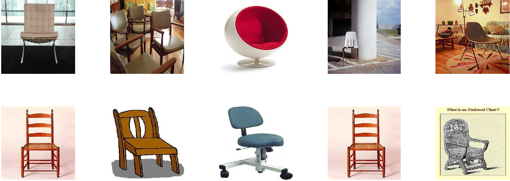
A visual example where we classify ImageNet images using models trained on Caltech-256 images is shown in Figure 2 and Figure 3. The nearest neighbor coming from Caltech-256 corresponds to the same class, even though the appearance of images are very different for the two datasets.
In Table 5 we report results using a SVM classifier for the unsupervised DA setting. In this case our method systematically outperforms all other DA methods, confirming the good behavior of our approach.
| Method | LC | LI | CL | CI | IL | IC | AVG |
|---|---|---|---|---|---|---|---|
| NA | 46.0 | 38.4 | 29.5 | 31.3 | 36.9 | 45.5 | 37.9 |
| Baseline-S | 24.2 | 27.2 | 46.9 | 41.8 | 35.7 | 33.8 | 34.9 |
| Baseline-T | 24.6 | 27.4 | 47.0 | 42.0 | 35.6 | 33.8 | 35.0 |
| GFK | 24.2 | 26.8 | 44.9 | 40.7 | 35.1 | 33.8 | 34.3 |
| TCA | 25.7 | 27.5 | 43.1 | 38.8 | 29.6 | 26.8 | 31.9 |
| SA | 49.1 | 41.2 | 47.0 | 39.1 | 39.4 | 54.5 | 45.0 |
| Method | LC | LI | CL | CI | IL | IC | AVG |
|---|---|---|---|---|---|---|---|
| NA | 49.6 | 40.8 | 36.0 | 45.6 | 41.3 | 58.9 | 45.4 |
| Baseline-S | 50.5 | 42.0 | 39.1 | 48.3 | 44.0 | 59.7 | 47.3 |
| Baseline-T | 48.7 | 41.9 | 39.2 | 48.4 | 43.6 | 58.0 | 46.6 |
| GFK | 52.3 | 43.5 | 39.6 | 49.0 | 45.3 | 61.8 | 48.6 |
| TCA | 46.7 | 39.4 | 37.9 | 47.2 | 41.0 | 56.9 | 44.9 |
| SA | 52.9 | 43.9 | 43.8 | 50.9 | 46.3 | 62.8 | 50.1 |
All these results suggest that classifying Caltech-256 images from various other sources seems a difficult task for most of the methods (–see Table 2 and Table 4). By analyzing results from section 4.5.2, we can see that ImageNet is a good source to classify images from Caltech-256 and LabelMe datasets.
4.5.3 Classifying PASCAL-VOC-2007 images using classifiers trained on ImageNet
In this experiment, we compare the average precision obtained on PASCAL-VOC-2007 by a SVM classifier in an unsupervised DA setting. We use ImageNet as the source domain and PASCAL-VOC-2007 as the target domain. The results are shown in Figure 6.
Our method achieves the best results for all the categories, GFK improves by 7% in mAP over no adaptation while our method improves by 27% in mAP over GFK.
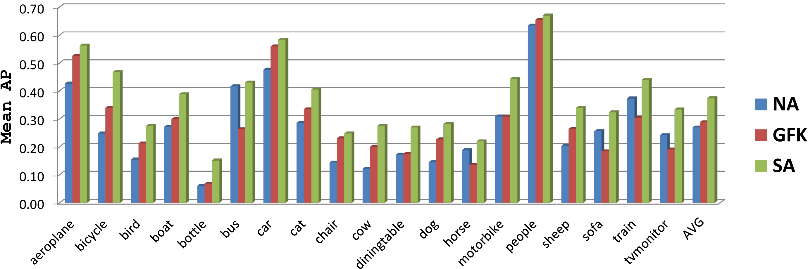
In section 4.5.1,4.5.2 and 4.5.3 we evaluate several domain adaptation algorithms using both NN and SVM classifiers. In all three cases, SA method outperforms TCA, GFS, GFK and baseline methods. The target accuracy obtained with the NN classifier is comparable with the ones obtained with the SVM classifier for Office+Caltech10 dataset. On the other hand for dataset all methods get a boost in results when used with an SVM classifier. As a result in the rest of the experiments we use NN classifier whenever we use Office+Caltech10 dataset for evaluation.
4.6 Evaluating methods that use source labels during DA
In this section we evaluate the effect of supervised ITML-PCA subspace creation method presented in section 3.4 and the large margin subspace alignment (LMSA) method introduce in section 3.5. For this experiment we use the Office-Caltech-10 dataset. We compare several supervised subspace-based DA methods in Table 6, namely PLS, LDA and ITML-PCA method introduce in section 3.4.
| Method | CA | DA | WA | AC | DC | WC | |
|---|---|---|---|---|---|---|---|
| GFK (PLS,PCA) | 40.4 | 36.2 | 35.5 | 37.9 | 32.7 | 29.3 | |
| GFK (LDA,PCA) | 41.6 | 36.2 | 39.9 | 31.9 | 31.0 | 36.7 | |
| GFK (ITML-PCA,PCA) | 41.0 | 34.9 | 40.3 | 39.2 | 35.4 | 36.0 | |
| SA (PLS,PCA) | 32.0 | 32.0 | 31.0 | 32.8 | 29.8 | 24.8 | |
| SA (LDA,PCA) | 48.3 | 37.6 | 41.6 | 35.7 | 34.3 | 39.2 | |
| SA (ITML-PCA,PCA) | 47.1 | 40.0 | 42.4 | 41.1 | 38.1 | 39.8 | |
| LMSA | 45.9 | 36.9 | 43.6 | 40.0 | 35.6 | 40.4 | |
| Method | AD | CD | WD | AW | CW | DW | AVG. |
| GFK (PLS,PCA) | 35.1 | 41.1 | 71.2 | 35.7 | 35.8 | 79.1 | 42.5 |
| GFK (LDA,PCA) | 35.5 | 37.1 | 68.9 | 37.0 | 37.1 | 76.9 | 42.5 |
| GFK (ITML-PCA,PCA) | 35.5 | 35.1 | 74.6 | 36.1 | 36.0 | 79.8 | 43.7 |
| SA (PLS,PCA) | 32.3 | 35.4 | 71.1 | 34.0 | 34.1 | 75.0 | 38.7 |
| SA (LDA,PCA) | 32.0 | 34.0 | 58.6 | 35.2 | 46.0 | 73.6 | 43.0 |
| SA (ITML-PCA,PCA) | 43.7 | 40.4 | 83.0 | 43.5 | 42.8 | 84.5 | 48.9 |
| LMSA | 41.4 | 44.1 | 76.4 | 40.4 | 40.4 | 81.1 | 47.2 |
As can be seen from the Table 6, SA(ITML-PCA,PCA) performs
better than SA(LDA,PCA) and SA(PLS,PCA).
SA(LDA,PCA) reports on average a
mean accuracy of 43.0% over 12 DA problems while the SA(ITML-PCA,PCA)
method reports the best mean accuracy of 48.5 %. ITML-PCA method also
improves GFK results by 1.2% showing the general applicability of this
approach. GFK(PLS,PCA) and GFK(LDA,PLS) report a mean accuracy of 42.5%
while GFK(ITML-PCA,PCA) reports an accuracy of 43.7 %. This clearly
shows that the (ITML-PCA) strategy obtains better results for GFK as
well as for the SA method. SA(PLS,PCA) reports a very poor accuracy of
38.7%. This could be due to the fact that when PLS is used, the upper
bound obtained by consistency theorem does not hold anymore and we
are likely to obtain a subspace dimension that only works in the
source domain. In contrast, the ITML-PCA method still uses PCA
to create a linear subspace and so the consistency theorem holds.
ITML uses both similarity and dissimilarity constraints using an information theoretic procedure. The learned metric in Algorithm (2) is regularized by regularization during the ITML procedure. The metric learning objective makes the subspace discriminative while allowing the domain transfer using SA method. From this result we conclude that is a better approach for subspace alignment-based domain adaptation as well as GFK method. In future work we plan to incorporate ITML [9] like objective directly in the subspace alignment objective function similar to LMSA method.
4.7 Evaluating SA-MLE method using high dimensional data
| Method | D W | W D | A W | AVG |
| NA | 62.7 1.1 | 64.7 2.2 | 17.1 2.1 | 48.2 1.7 |
| SA | 71.6 0.9 | 70.6 1.6 | 17.0 1.6 | 53.1 1.8 |
| SA-MLE | 68.92.1 | 68.0 1.3 | 16.7 1.4 | 51.2 1.6 |
Despite having a large dimensionality, Fisher vectors [23] have proven to be a robust image representation for image classification task. One limitation of subspace alignment is the computational complexity associated with high dimensional data (see section 3.3.2). We overcome this issue using SA-MLE method.
In this experiment we also use the Office dataset [24] as well as the Office+Caltech-10 dataset. The reason is that the Office dataset consists of more object classes and images (even though it has only three domains). We extract SURF [2] features to create a Gaussian mixture model (GMM) of 64 components and encode images using Fisher encoding [23]. The GMM is created from Amazon images from the Office dataset.
Results on the Office dataset using Fisher vectors are shown in Table 7 while in Table 8 results for Office+Caltech-10 is reported. These results indicate the effectiveness of SA-MLE method considering the fact that it can estimate the subspace dimensionality almost 100 times faster than SA method when used with Fisher vectors. On average, SA-MLE outperforms no adaptation (NA) results. Since MLE method returns two different subspace dimensionality for the source and the target, it is not clear how we can apply MLE method on GFK.
Note that SA-MLE is fast and operates in the low-dimensional target subspace. More importantly SA-MLE seems to work well with Fisher vectors. The computational complexity of SA-MLE equal to where is the target subspace dimensionality. On the other hand, an estimate of the computational complexity of SA is due to the cross validation procedure necessary to establish the optimal subspace dimensionality. Given the fact that SA-MLE is way faster than SA method and obtain reasonable results, we recommend SA-MLE for real time DA methods. Also we recommend to use SA-MLE method if the dimensionality of data is larger and when computational time is an issue.
| Method | C A | DA | WA | AC | DC | WC | AD | CD | WD | AW | CW | DW | AVG |
| NA | 44.3 | 35.7 | 34.2 | 36.9 | 33.9 | 30.8 | 37.4 | 42.1 | 76.7 | 35.2 | 32.2 | 82.7 | 43.5 |
| SA | 48.2 | 44.6 | 43.1 | 40.3 | 38.4 | 35.9 | 45.0 | 51.6 | 87.6 | 44.8 | 44.4 | 90.1 | 51.2 |
| SA-MLE | 48.0 | 39.0 | 40.0 | 39.9 | 37.5 | 33.0 | 43.9 | 50.8 | 86.3 | 40.7 | 40.5 | 88.7 | 49.0 |
4.8 Effect of dictionary size on domain adaptation
In this experiment we change the dictionary size of BOVW image representation and evaluate the performance on the target domain. For this experiment we use the Office-Caltech dataset. The dictionary is created using SURF features extracted from Amazon images (10 classes) of the Office dataset using the k-means algorithm. The subspace is created using PCA (no ITML is applied). For this experiment we use all source images for training and test on all target images. We compute the average accuracy using NN classifier over all 12 domain adaptation problems for each considered method and plot the mean accuracy in Fig. 7.

From Fig. 7, we see clearly, the visual dictionary size affects the magnitude of domain shift. We can conclude that as the dictionary size increases the performance of the target domain increases up-to a point and then starts to drop for NA, Baseline-T and GFK. SA method performs the best for all dictionary sizes. The typical dictionary size used in the literature for this dataset is 800 visual words. But it seems that larger visual dictionary of 2048 words or beyond works the best for subspace based DA methods such as TCA, GFK and SA. This indicates that image representation can influence different domain adaptation methods differently.
4.9 The effect of deep learning features for subspace based DA
The divergence between domains depends on the representation used [3]. In this experiment we compare the classification performance on the target domain using the state of the art image classification feature called Decaf [10]. Decaf uses deep learning [15] based approach.
We compare the performance of subspace based DA methods using the nearest neighbor classifier and SVM classifier. For this experiment we use the more challenging Office dataset which consists of 31 object classes and three domains (Amazon, Webcam and DSLR). We show results for NA, GFK, TCA and SA methods using DECAF features in Table 9 for NN classifier and in Table 10 for SVM classifier.
| Method | DW | WD | AW |
| NA | 86.4 1.1 | 88.6 1.2 | 42.8 0.9 |
| GFK | 69.2 2.1 | 61.8 2.3 | 39.5 2.1 |
| TCA | 57.1 1.7 | 51.1 1.8 | 24.8 3.2 |
| SA | 86.8 1.0 | 89.3 0.8 | 44.7 0.7 |
| Method | DW | WD | AW |
| NA | 91.3 1.2 | 91.6 1.6 | 47.9 2.9 |
| GFK | 87.2 1.3 | 88.1 1.5 | 46.8 1.8 |
| TCA | 89.0 1.4 | 87.9 1.9 | 44.6 3.0 |
| SA | 91.8 0.9 | 92.4 1.7 | 47.2 1.5 |
Results in Table 9 suggest that there is a slight advantage of SA method over all domains. On the other-hand GFK and TCA seem to perform very poorly. When used with SVM classifier both GFK and TCA perform much better than with NN classifier (–see Table 10). Clearly, the DECAF features boost the performance in typical DA datasets such as Office. However, we notice that the performance for DA problem is lower. All subspace-based DA methods have low-performance for this DA problem when SVM classifier is used. However, SA seems to improve over DECAF features for this DA task when NN classifier is utilized. We believe there is still room for improvements for DA methods to boost recognition rate when DECAF is used as a representation.
DECAF being a deep learning feature, it is trained from millions of images in a discriminative manner. From learning theory point of view, this allows to attenuate the probabilistic upper bound on classification error in the test set. At the same time, probably as millions of images are used during the training, it is possible that training algorithms (Convolutional neural network + upper layers) has already visited variety of images from different domains allowing the learning algorithm to be invariant to differences in domains and build a representation that is quite domain invariant in general.
4.10 Effect of z-normalization
As we mentioned in section 3.1, z-normalization influences DA methods such as GFK, TCA and SA. To evaluate this, we perform an experiment using Office+Caltech-10 dataset. In this experiment we use all source data for training and all target data for testing. We use the same BOW features as in [12]. We report mean accuracy over 12 domain adaptation problems in Fig. 8. We report accuracy with and without z-normalization for all considered DA methods.

It is clear that all DA method including the methods such as projecting to the source (Baseline-S) and target domain (Baseline-T) hugely benefited by the z-normalization. The biggest beneficiary is the TCA method while GFK as well as most other methods even fail to improve over no adaptation without z-normalization. SA method is benefited from z-normalization but even without z-normalization it improves over NA results.
4.11 Comparison with other non-subspace-based DA methods
In this section we compare our method with several non-subspace based domain adaptation methods that exist in the literature. For this evaluation we use the Office+Caltech-10 dataset(–see Table 11). We compare with traditional self-labeling method similar to DA-SVM [34], KLIEP-based [36] instance weighting DA method and a dictionary learning based DA method [35]. From results in Table 11, it is interesting to see that simple Self-labeling methods seems to work well on this dataset. Especially, for DA tasks such as and self-labeling seems to outperforms SA method. The instance weighting method based on KLIEP [36] algorithm did not perform well on this dataset. On the other-hand, methods based on dictionary learning seems to work better than SA for some problems such as and . We believe that a combination of all these methods might lead to superior performance. In theory, SA method can be combined with instance weighting, self-labeling and dictionary learning based methods. Such a combination of strategies might assist to overcome practical domain shift issues in application areas such as video surveillance and vision-based-robotics. In future, we plan to investigate the applicability of such combination of strategies in real-world DA scenarios.
| Method | CA | DA | WA | AC | DC | WC | AD | CD | WD | AW | CW | DW | AVG. |
| SA (ITML-PCA,PCA) | 47.1 | 40.0 | 42.4 | 41.1 | 38.1 | 39.8 | 43.7 | 40.4 | 83.0 | 43.5 | 42.8 | 84.5 | 48.5 |
| Self-labelling (SVM) | 52.1 | 37.7 | 36.2 | 38.3 | 28.2 | 28.3 | 40.2 | 41.3 | 70.9 | 39.0 | 46.7 | 81.2 | 45.0 |
| Instance Wighting (LKIEP+SVM) | 43.2 | 34.9 | 30.4 | 36.0 | 31.0 | 23.1 | 24.3 | 28.0 | 36.7 | 27.3 | 28.2 | 66.4 | 34.1 |
| Dictionary Learning [35] | 45.4 | 39.1 | 38.3 | 40.4 | N/A | 36.3 | N/A | 42.3 | N/A | 37.9 | N/A | 86.2 | 45.7 |
5 Discussion and Conclusion
We have presented a new visual domain adaptation method using subspace alignment. In this method, we create subspaces for both source and target domains and learn a linear mapping that aligns the source subspace with the target subspace. This allows us to compare the source domain data directly with the target domain data and to build classifiers on source data and apply them on the target domain. We demonstrate excellent performance on several image classification datasets such as Office dataset, Caltech, ImageNet, LabelMe and Pascal-VOC2007. We show that our method outperforms state-of-the-art domain adaptation methods using both SVM and nearest neighbour classifiers. Due to its simplicity and theoretically founded stability, our method has the potential to be applied on large datasets. For example, we use SA to label PASCAL-VOC2007 images using the classifiers build on ImageNet dataset.
In this extended version of our original work, we addressed several limitations of our previous paper. First, we propose SA-MLE method which does not require any cross-validation to find the optimal subspace dimensionality. SA-MLE uses maximum likelihood estimation to find a good source and target subspace dimensionality. Secondly, we propose a new way to use label information of the source domain to obtain more discriminative source subspace. Thirdly, we provided some analysis on domain adaptation from representation point of view. We showed that the dictionary size of the bag-of-words representation influences the classification performance of subspace-based DA methods. Generally, larger visual vocabulary seems to improve domain adapted results even when results without adaptation is significantly low. At the same time we see that new representations such as DECAF can be used to improve recognition rates over different domains. We conclude that visual domain adaptation can be overcome by either choosing generic image representations or by developing better DA algorithms such as subspace alignment.
Our method assumes that both the source and the target data lie in the same space and joint distributions to be correlated. SA method exploits this correlation, if there is any to do the adaptation. If both joint-distributions are independent, then it would be impossible for our method to learn any meaningful adaptation.
The subspace alignment method assumes both source and target domain have similar class prior probability distributions. When there is significant change in class prior probability (as recently discussed in target shifts [31]), the subspace alignment method may fail. Also in future work we plan to incorporate information theoretic metric learning like domain constraints directly in the subspace alignment objective function.
Acknowledgements:
The authors acknowledge the support of the FP7 ERC Starting Grant 240530
COGNIMUND, ANR LAMPADA 09-EMER-007-02 project and PASCAL 2 network of
Excellence.
References
- [1] Baktashmotlagh, M., Harandi, M.T., Lovell, B.C., Salzmann, M.: Unsupervised domain adaptation by domain invariant projection. In: The IEEE International Conference on Computer Vision (ICCV) (2013)
- [2] Bay, H., Ess, A., Tuytelaars, T., Van Gool, L.: Speeded-up robust features (surf). Comput. Vis. Image Underst. 110(3), 346–359 (2008). DOI 10.1016/j.cviu.2007.09.014. URL http://dx.doi.org/10.1016/j.cviu.2007.09.014
- [3] Ben-David, S., Blitzer, J., Crammer, K., Pereira, F.: Analysis of representations for domain adaptation. In: NIPS. NIPS (2007)
- [4] Ben-David, S., Shalev-Shwartz, S., Urner, R.: Domain adaptation–can quantity compensate for quality? In: International Symposium on Artificial Intelligence and Mathematics (2012)
- [5] Blitzer, J., Foster, D., Kakade, S.: Domain adaptation with coupled subspaces. In: Conference on Artificial Intelligence and Statistics. Fort Lauterdale (2011)
- [6] Blitzer, J., McDonald, R., Pereira, F.: Domain adaptation with structural correspondence learning. In: Conference on Empirical Methods in Natural Language Processing (2006)
- [7] Chang, S.F.: Robust visual domain adaptation with low-rank reconstruction. In: CVPR (2012). URL http://dl.acm.org/citation.cfm?id=2354409.2355115
- [8] Chen, B., Lam, W., Tsang, I., Wong, T.L.: Extracting discriminative concepts for domain adaptation in text mining. In: ACM SIGKDD (2009)
- [9] Davis, J.V., Kulis, B., Jain, P., Sra, S., Dhillon, I.S.: Information-theoretic metric learning. In: Proceedings of the 24th International Conference on Machine Learning, ICML ’07, pp. 209–216. ACM, New York, NY, USA (2007)
- [10] Donahue, J., Jia, Y., Vinyals, O., Hoffman, J., Zhang, N., Tzeng, E., Darrell, T.: Decaf: A deep convolutional activation feature for generic visual recognition. CoRR abs/1310.1531, 1–8 (2013)
- [11] Fernando, B., Habrard, A., Sebban, M., Tuytelaars, T., et al.: Unsupervised visual domain adaptation using subspace alignment. In: ICCV (2013)
- [12] Gong, B., Shi, Y., Sha, F., Grauman, K.: Geodesic flow kernel for unsupervised domain adaptation. In: CVPR (2012)
- [13] Gopalan, R., Li, R., Chellappa, R.: Domain adaptation for object recognition: An unsupervised approach. In: ICCV (2011)
- [14] Khosla, A., Zhou, T., Malisiewicz, T., Efros, A.A., Torralba, A.: Undoing the damage of dataset bias. In: ECCV (2012)
- [15] Krizhevsky, A., Sutskever, I., Hinton, G.E.: Imagenet classification with deep convolutional neural networks. In: NIPS, vol. 1, p. 4 (2012)
- [16] Kulis, B., Saenko, K., Darrell, T.: What you saw is not what you get: Domain adaptation using asymmetric kernel transforms. In: CVPR (2011). DOI 10.1109/CVPR.2011.5995702. URL http://dx.doi.org/10.1109/CVPR.2011.5995702
- [17] Levina, E., Bickel, P.J.: Maximum likelihood estimation of intrinsic dimension. In: NIPS (2004)
- [18] Van der Maaten, L., Hinton, G.: Visualizing data using t-sne. Journal of Machine Learning Research 9(11), 1–8 (2008)
- [19] Margolis, A.: A literature review of domain adaptation with unlabeled data. Tech. rep., University of Washington (2011)
- [20] Pan, S.J., Kwok, J.T., Yang, Q.: Transfer learning via dimensionality reduction. In: AAAI (2008)
- [21] Pan, S.J., Tsang, I.W., Kwok, J.T., Yang, Q.: Domain adaptation via transfer component analysis. In: IJCAI (2009)
- [22] Patel, V.M., Gopalan, R., Li, R., Chellappa, R.: Visual domain adaptation: An overview of recent advances. Submitted 1, 1–8 (2014)
- [23] Perronnin, F., Liu, Y., Sánchez, J., Poirier, H.: Large-scale image retrieval with compressed fisher vectors. In: Computer Vision and Pattern Recognition (CVPR), 2010 IEEE Conference on, pp. 3384–3391. IEEE (2010)
- [24] Saenko, K., Kulis, B., Fritz, M., Darrell, T.: Adapting visual category models to new domains. In: ECCV (2010)
- [25] Shao, M., Kit, D., Fu, Y.: Generalized transfer subspace learning through low-rank constraint. International Journal of Computer Vision pp. 1–20 (2014)
- [26] Torralba, A., Efros, A.: Unbiased look at dataset bias. In: CVPR (2011)
- [27] Wang, C., Mahadevan, S.: Manifold alignment without correspondence. In: IJCAI (2009)
- [28] Wang, C., Mahadevan, S.: Heterogeneous domain adaptation using manifold alignment. In: IJCAI (2011)
- [29] Weinberger, K.Q., Saul, L.K.: Distance metric learning for large margin nearest neighbor classification. J. Mach. Learn. Res. 10, 207–244 (2009)
- [30] Zhai, D., Li, B., Chang, H., Shan, S., Chen, X., Gao, W.: Manifold alignment via corresponding projections. In: BMVC (2010)
- [31] Zhang, K., Muandet, K., Wang, Z., et al.: Domain adaptation under target and conditional shift. In: ICML, pp. 819–827 (2013)
- [32] Zwald, L., Blanchard, G.: On the convergence of eigenspaces in kernel principal components analysis. In: NIPS (2005)
- [33] Bellet, A.,Habrard, A.,Sebban, M.: A Survey on Metric Learning for Feature Vectors and Structured Data. In: CoRR (2013)
- [34] Bruzzone, L., Marconcini, M.: Domain Adaptation Problems: A DASVM Classification Technique and a Circular Validation Strategy. PAMI 32, 770–787 (2010)
- [35] Jie Ni, Qiang Qiu, and Rama Chellappa. Subspace interpolation via dictionary learning for unsupervised domain adaptation. In CVPR, June 2013.
- [36] Sugiyama .M, Nakajima S., Kashima H., von Bünau P., Kawanabe M. : Direct importance estimation with model selection and its application to covariate shift adaptation. In NIPS, 2007.