Deep Regression for Face Alignment

The architecture of the global layer is depicted in Figure 1.b. The global layer predicts the initial shape estimation $\mathbf{s}^{0}$ from the global feature of image ${I}$. We use linear regression for this layer and predict the initial shape $\mathbf{s}^{0}$ directly from the global image features $\boldsymbol{\upphi}^{0}$:

where $g(\cdot)$ extracts a $d_{0}$-dimensional global features $\boldsymbol{\upphi}^{0}$ from an image, $GR(\cdot)$ represents the global regression function, $\mathbf{W}^{0}\in\Re^{2P\times d_{0}}$ is the linear regression coefficient matrix, and $\mathbf{b}^{0}$ is the bias vector. For clarity, the later presentation will drop this bias term in the regression function.

The linear regressor with the global feature gives a coarse estimation of the shape, which, however, is already a good initialization for the following local layers.

Each local layer refines the shape estimated from the previous layer. The architecture of the $t$-th local layer is depicted in Figure 1.b. It extracts the local (shape-indexed) feature $\boldsymbol{\upphi}^{t}$ and use it to predict the shape increment $\Delta\mathbf{s}^{t}$ using a linear regressor. The increment is added to $\mathbf{s}^{t-1}$ from the previous layer to produce the refined shape estimation $\mathbf{s}^{t}$. In mathematical form:

where $h:I,\mathbf{s}^{t-1}\rightarrow\boldsymbol{\upphi}^{t}\in\Re^{d_{t}}$ is the local feature extraction function, $LR(\cdot,\cdot)$ represents the local regression function, $\mathbf{W}^{t}\in\Re^{2P\times d_{t}}$ is the linear regression matrix for the $t$-th local regressor. $\boldsymbol{\upphi}^{t}$ is constructed by concatenating local descriptors around each landmark: $\boldsymbol{\upphi}^{t}=[{\boldsymbol{\upphi}_{1}^{t}}^{\intercal},{\boldsymbol{\upphi}_{2}^{t}}^{\intercal},\dots,{\boldsymbol{\upphi}_{P}^{t}}^{\intercal}]^{\intercal}$, $\boldsymbol{\upphi}_{p}^{t}$ is the descriptor extracted around the $p$-th landmark.

Local regressors extract features that describe local appearance and is more suitable for finer adjustment of landmark positions. Besides, it uses only a subset of image pixels for feature extraction and is more advantageous on computational efficiency.

Sequential learning computes the regression coefficients one by one from $\mathbf{W}^{0}$ to $\mathbf{W}^{T}$ to approximately minimize the objective function $E(\theta)$. The regression coefficient for each regressor is optimized, by fixing the trained regression coefficients of the regressors preceding it and minimizing the difference of its predicted shape from the true shape.

The coefficient matrix $\mathbf{W}^{0}$ of the global regressor is solved as

The coefficient matrix $\mathbf{W}^{t}$ of the $t$th local regressor is solved as

where $\boldsymbol{\upphi}_{i}^{t}=h(I_{i},\mathbf{s}^{t-1}_{i})$ and $\mathbf{s}^{t-1}_{i}$ are fixed given the coefficients of the first $t$ regressors are estimated.

The sequential learning algorithm is clearly sub-optimal as the coefficient matrix estimation of each regressor does not exploit the later regressors. Empirically, we observe that the first few regressors make greater paces to approach the true shape, i.e., smaller bias of the shape estimation from those regressors, while the latter regressors make smaller paces. Importantly, we find that the shape estimation from the first regressors has larger estimation variances. This results in the variance of the local (shape-indexed) features is also larger. As a consequence, it is harder for the later regressors to make a good shape estimation.

In the following, we will introduce the joint learning algorithm using back-propagation to directly optimize the objective function such that the optimization of the regression coefficient matrix helps each other. The empirical results show that joint learning is able to make a balanced optimization of the bias and the variance of the shape estimation from the regressors: both the bias and the variance gradually decrease from the early regressors to the later regressors. Consequently, joint learning yields a better whole shape estimation. Figure 2 illustrates the performance comparison of each regressors using sequential learning and joint learning.

We adopt the gradient descent method to jointly estimate the regression coefficient matrices by minimizing the global error function $E(\theta)$. We apply the back-propagation algorithm [20] to efficiently the evaluate derivatives of the error function with respect to the coefficient matrices.

The derivatives of local layers. The partial derivatives of the error function with respect to $\mathbf{W}^{t}$ and $\mathbf{s}^{t}$ are computed using the backward recurrence as:

According to Equation 2, $\frac{\partial E}{\partial\mathbf{W}^{t}}=\boldsymbol{\upphi}^{t}\frac{\partial E}{\partial\mathbf{s}^{t}}$. The partial derivatives $\frac{\partial LR^{t}}{\partial\mathbf{s}^{t-1}}$ are computed as:

where $\mathbf{I}\in\Re^{2P\times 2P}$ is an identity matrix, and $\frac{\partial h}{\partial\mathbf{s}^{t-1}}$ is the partial derivative of the local feature extractor with respect to the shape vector $\mathbf{s}^{t-1}$.

The derivatives of local feature extractors. The Jacobian matrix of the function $h(I,\mathbf{s})$ with respect to the shape $\mathbf{s}$ is denoted by $\boldsymbol{\uppsi}=\frac{\partial h}{\partial\mathbf{s}}$. For simplicity, we drop the superscript $t$. $h(I,\mathbf{s})$ is the local feature extraction operation and is non-differentiable, and thus its gradients cannot be calculated analytically. We numerically approximate $\boldsymbol{\uppsi}$ by computing the second-order approximation:

where $\mathbf{s}^{j+}$ and $\mathbf{s}^{j-}$ are equal to $\mathbf{s}$ except the $j$-th dimension, where $\mathbf{s}_{j}^{j+}=\mathbf{s}_{j}+\epsilon$ and $\mathbf{s}_{j}^{j-}=\mathbf{s}_{j}-\epsilon$ respectively. The $\epsilon$ is chosen to be a small value which corresponds to several pixels in the image.

Since that $\boldsymbol{\upphi}=[\boldsymbol{\upphi}_{1}^{\intercal},\ \boldsymbol{\upphi}_{2}^{\intercal},\ \dots,\ \boldsymbol{\upphi}_{P}^{\intercal}]^{\intercal}$ is the concatenation of local descriptors extracted around $P$ landmarks, each dimension of $\boldsymbol{\upphi}$ is determined by the corresponding landmarks positions $x_{p},y_{p}$, which are two dimensions of $\mathbf{s}$. Therefore $\boldsymbol{\uppsi}$ is a block-diagonal matrix $\boldsymbol{\uppsi}=\mathop{\mathrm{diag}}(\boldsymbol{\uppsi}_{1},\boldsymbol{\uppsi}_{2},\dots,\boldsymbol{\uppsi}_{P})$ of which each block $\boldsymbol{\uppsi}_{p}=[\boldsymbol{\uppsi}_{px}\ \boldsymbol{\uppsi}_{py}]$. $\boldsymbol{\uppsi}_{px}$ and $\boldsymbol{\uppsi}_{py}$ are respectively the local descriptor gradients along the $x$ and $y$ axis, given by:

Here $h_{p}({I},x_{p},y_{p})$ is the local descriptor function on the $p$-th landmark whose coordinates are $x_{p},y_{p}$.

The derivatives of the global layer. The derivatives of the error function with respect to the regression coefficient matrix $\mathbf{W}^{0}$, according to Equation 1, are computed as follows:

Datasets: Performance is evaluated on the LFPW dataset [1] and the 300-W dataset [21]. The LFPW dataset is annotated by $29$ landmarks. The dataset provides URLs only and some are no longer valid. We use $717$ of the $1100$ images for training and $249$ of the $300$ images for testing. 300-W dataset is created from several re-annotated datasets including LFPW [1], AFW [28], Helen [12] and XM2VTS [17]. The number of landmarks is $68$. Since the official testing set of 300-W is not publicly available, we follow [19] and build the training set using AFW, the training set of LFPW and the training set of Helen, with $3148$ images in total. Our testing set consists of IBUG, the testing set of LFPW and the testing set of Helen, with 689 images in total. Also following [19], we evaluate performance on 1) all images of the testing set, called the Fullset 2) testing sets of Helen and LFPW, called the Common Subset and 3) IBUG dataset, called the Challenging Subset.

Evaluation metric: Following [1], we evaluate performance by the average landmark error normalized by inter-pupil distance:

where $\hat{x}_{p}^{(i)},\hat{y}_{p}^{(i)}$ are ground truth coordinates for the $p$-th landmark of the $i$-th sample, $d_{\textrm{pupils}}^{(i)}$ is the inter-pupil distance of the $i$-th sample. For 300-W, pupil landmarks are not annotated and are replaced by the mean landmarks of the landmarks around each eye.

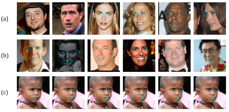
We term our approach as DeepReg, our approach with sequential learning as SequentialReg and a variant of the network which drops the global regressor as DeepRegLocal. The initial shape estimation $\mathbf{s}^{0}$ in DeepRegLocal is given by the mean shape $\bar{\mathbf{s}}$ calculated from the training set, as adopted in cascaded regression [25, 2, 19]. First, we compare the result of DeepReg with the two baseline algorithms: SequentialReg and DeepRegLocal. The results are listed in Table 1 and visualized in Figure 3.

One can see from Table 1 that DeepReg outperforms both SequentialReg and DeepRegLocal. The superiority over SequentialReg stems from joint optimization, which is able to balance the biases and the variances of all the regressors. The superiority over DeepRegLocal is because the global regressor is helpful to generate a robust initialization. Second, in comparison with the closely-related regression algorithm, supervised descent method (SDM, [25]), our approach performs better. The superiority of our approach and DeepRegLocal is not as significant as that to SequentialReg. The reason is that SDM did good job on feature transform, which potentially can help our approach, for example, including feature transform and even convolutions into our deep regress framework. Last, we also report the comparison results with other state-of-the-art algorithms, including the algorithm using a consensus of exemplars (CoE [1]), explicit shape regression (ESR [3]), robust cascaded pose regression (RCPR [2]) and local binary features (LBF [19]), in which our approach and LBF perform the best. As shown in Table 1, our approach performs better in 300-W Fullset and 300-W Common Subset over LBF, but poorer in LFPW and 300-W Challenging Subset. The reason is that LBF performs an extra feature learning step that is essential for good performance, and in essence our approach is able to benefit from this step if we can reproduce their reported results.

Figure 4 plots the estimation errors of all stages on the training, validation and testing sets. One can see from the plot that sequential learning tends to result in strong early stages which eliminate most of the error. The later stages, however, are much weaker. Joint learning mitigates this and the estimation gradually and evenly approaches the ground truth, resulting in a flattened error curve and better estimation eventually. Furthermore, as shown in Figure 2, joint learning balances between bias and variance and makes them gradually and simultaneously decrease, while in sequential learning the variance decreases much slower.

References

- [1] Peter N Belhumeur, David W Jacobs, D Kriegman, and Neeraj Kumar. Localizing parts of faces using a consensus of exemplars. In Computer Vision and Pattern Recognition (CVPR), 2011 IEEE Conference on, pages 545–552. IEEE, 2011.
- [2] Xavier P Burgos-Artizzu, Pietro Perona, and Piotr Dollár. Robust face landmark estimation under occlusion. ICCV, 2013.
- [3] Xudong Cao, Yichen Wei, Fang Wen, and Jian Sun. Face alignment by explicit shape regression. International Journal of Computer Vision, 107(2):177–190, 2014.
- [4] Timothy F Cootes, Gareth J Edwards, Christopher J Taylor, et al. Active appearance models. IEEE Transactions on pattern analysis and machine intelligence, 23(6):681–685, 2001.
- [5] Timothy F Cootes, Christopher J Taylor, David H Cooper, and Jim Graham. Active shape models-their training and application. Computer vision and image understanding, 61(1):38–59, 1995.
- [6] David Cristinacce and Timothy F Cootes. Boosted regression active shape models. In BMVC, pages 1–10, 2007.
- [7] Navneet Dalal and Bill Triggs. Histograms of oriented gradients for human detection. In Computer Vision and Pattern Recognition, 2005. CVPR 2005. IEEE Computer Society Conference on, volume 1, pages 886–893. IEEE, 2005.
- [8] Liya Ding and Aleix M Martinez. Precise detailed detection of faces and facial features. In Computer Vision and Pattern Recognition, 2008. CVPR 2008. IEEE Conference on, pages 1–7. IEEE, 2008.
- [9] Piotr Dollár, Peter Welinder, and Pietro Perona. Cascaded pose regression. In Computer Vision and Pattern Recognition (CVPR), 2010 IEEE Conference on, pages 1078–1085. IEEE, 2010.
- [10] Geoffrey E Hinton, Nitish Srivastava, Alex Krizhevsky, Ilya Sutskever, and Ruslan R Salakhutdinov. Improving neural networks by preventing co-adaptation of feature detectors. arXiv preprint arXiv:1207.0580, 2012.
- [11] Alex Krizhevsky, Ilya Sutskever, and Geoffrey E Hinton. Imagenet classification with deep convolutional neural networks. In NIPS, volume 1, page 4, 2012.
- [12] Vuong Le, Jonathan Brandt, Zhe Lin, Lubomir Bourdev, and Thomas S Huang. Interactive facial feature localization. In Computer Vision–ECCV 2012, pages 679–692. Springer, 2012.
- [13] Yann A LeCun, Léon Bottou, Genevieve B Orr, and Klaus-Robert Müller. Efficient backprop. In Neural networks: Tricks of the trade, pages 9–48. Springer, 2012.
- [14] Lin Liang, Rong Xiao, Fang Wen, and Jian Sun. Face alignment via component-based discriminative search. In Computer Vision–ECCV 2008, pages 72–85. Springer, 2008.
- [15] David G Lowe. Distinctive image features from scale-invariant keypoints. International journal of computer vision, 60(2):91–110, 2004.
- [16] Iain Matthews and Simon Baker. Active appearance models revisited. International Journal of Computer Vision, 60(2):135–164, 2004.
- [17] Kieron Messer, Jiri Matas, Josef Kittler, Juergen Luettin, and Gilbert Maitre. Xm2vtsdb: The extended m2vts database. In Second international conference on audio and video-based biometric person authentication, volume 964, pages 965–966. Citeseer, 1999.
- [18] Fatih Porikli. Integral histogram: A fast way to extract histograms in cartesian spaces. In Computer Vision and Pattern Recognition, 2005. CVPR 2005. IEEE Computer Society Conference on, volume 1, pages 829–836. IEEE, 2005.
- [19] Shaoqing Ren, Xudong Cao, Yichen Wei, and Jian Sun. Face alignment at 3000 fps via regressing local binary features. In Computer Vision and Pattern Recognition (CVPR), 2014 IEEE Conference on. IEEE, 2014.
- [20] David E Rumelhart, Geoffrey E Hinton, and Ronald J Williams. Learning representations by back-propagating errors. MIT Press, Cambridge, MA, USA, 1988.
- [21] Christos Sagonas, Georgios Tzimiropoulos, Stefanos Zafeiriou, and Maja Pantic. A semi-automatic methodology for facial landmark annotation. In Computer Vision and Pattern Recognition Workshops (CVPRW), 2013 IEEE Conference on, pages 896–903. IEEE, 2013.
- [22] Yi Sun, Xiaogang Wang, and Xiaoou Tang. Deep convolutional network cascade for facial point detection. In Computer Vision and Pattern Recognition (CVPR), 2013 IEEE Conference on, pages 3476–3483. IEEE, 2013.
- [23] Ilya Sutskever, James Martens, George Dahl, and Geoffrey Hinton. On the importance of initialization and momentum in deep learning. In Proceedings of the 30th International Conference on Machine Learning (ICML-13), pages 1139–1147, 2013.
- [24] Engin Tola, Vincent Lepetit, and Pascal Fua. Daisy: An efficient dense descriptor applied to wide-baseline stereo. Pattern Analysis and Machine Intelligence, IEEE Transactions on, 32(5):815–830, 2010.
- [25] Xuehan Xiong and Fernando De la Torre. Supervised descent method and its applications to face alignment. In Computer Vision and Pattern Recognition (CVPR), 2013 IEEE Conference on, pages 532–539. IEEE, 2013.
- [26] Alan L Yuille, Peter W Hallinan, and David S Cohen. Feature extraction from faces using deformable templates. International journal of computer vision, 8(2):99–111, 1992.
- [27] Erjin Zhou, Haoqiang Fan, Zhimin Cao, Yuning Jiang, and Qi Yin. Extensive facial landmark localization with coarse-to-fine convolutional network cascade. In Computer Vision Workshops (ICCVW), 2013 IEEE International Conference on, pages 386–391. IEEE, 2013.
- [28] Xiangxin Zhu and Deva Ramanan. Face detection, pose estimation, and landmark localization in the wild. In Computer Vision and Pattern Recognition (CVPR), 2012 IEEE Conference on, pages 2879–2886. IEEE, 2012.