Risk-limiting Economic Dispatch for Electricity Markets with Flexible Ramping ProductsThanks: C. Wu, G. Hug and S. Kar are with the Department of Electrical and Computer Engineering, Carnegie Mellon University, Pittsburgh, PA 15213, USA, e-mails: chenyewu@andrew.cmu.edu, ghug@ece.cmu.edu, soummyak@andrew.cmu.edu.
Abstract
The expected increase in the penetration of renewables in the approaching decade urges the electricity market to introduce new products - in particular, flexible ramping products - to accommodate the renewables’ variability and intermittency. A risk-limiting economic dispatch scheme provides the means to optimize the dispatch and provision of these products. In this paper, we adopt the extended loss-of-load probability as the definition of risk. We first assess how the new products distort the optimal economic dispatch by comparing to the case without such products. Specifically, using parametric analysis, we establish the relationship between the minimal generation cost and the two key parameters of the new products: the up- and down-flexible ramping requirements. Such relationship yields a novel routine to efficiently solve the non-convex risk-limiting economic dispatch problem. Both theoretical analysis and simulation results suggest that our approach may substantially reduce the cost for incorporating the new products. We believe our approach can assist the ISOs with utilizing the ramping capacities in the system at the minimal cost.
Index Terms:
Flexible ramping product, real time market, renewable energy integration, parametric optimizationI Introduction
As the level of penetration of renewable generation (in particular wind and solar power) grows, the stochastic nature of the power outputs from these resources is increasingly stressing the power system. Hence, the NERC task force on the potential reliability impacts of emerging flexible resources [1] suggests designing new products for the future electricity market. These products should ensure sufficient ramping capacity to cope with large short-term variations and prediction errors [2]. Activity is starting to pick up: the California Independent System Operator (CAISO) [3] and the Midwest Independent System Operator (MISO) [4] are pioneering the design and have introduced flexible ramping products in their markets.
Conceptually, flexible ramping products aim at reserving ramping flexibility in the current time slot for future use. While frequency regulation already reserves certain flexibility to tackle unpredicted fluctuations in net load [5], the new products are expected to provide more flexibility than frequency regulation and on a much slower time scale (e.g., 5 minutes in CAISO). Spinning and non-spinning reserves are other existing products to provide flexibility but are held to manage system contingencies. Furthermore, they can only contribute to up-ramping flexibility while flexible ramping products are intended to tackle deviations in both directions.
Albeit promising and important, to better utilize these products, a risk-limiting economic dispatch scheme is warranted, in which we adopt the extended loss-of-load probability (LOLP) [6] as the definition of risk. The risk-limiting economic dispatch scheme is in general non-convex due to the constraints to limit the risk. This non-convexity heavily constrains the risk-limiting economic dispatch scheme from (near) real time implementation. We propose an efficient algorithm, which utilizes our understanding on how the new products distort the optimal economic dispatch compared to the market outcomes for the case without such products. The understanding is motivated by the following question: what are the main factors that determine the distortion?
Intuitively, it depends on how much ramping flexibility is needed. This value, on the other hand, is dependent on the desired level of reliability at which the load in the next time step should be supplied. In this paper, we adopt the risk-limiting constraint to enforce the desired level of supply reliability (or equivalently, LOLP). As different combinations of the up- and down-flexible ramping capacities may meet the same risk-limiting constraint, it is possible to optimize the combination by minimizing the total generation cost. We propose to solve this problem in two steps. First, by employing the theory of linear parametric programming [7], we propose a parametric functional approach to understand the dependency of the distortion cost on the level of up- and down-ramping requirements. Then, we introduce a linear search algorithm to solve the economic dispatch while guaranteeing a pre-defined risk-limiting constraint.
It is worth noting that the application of the proposed parametric analysis is not limited to the cost assessment. Examples of such application include: the parametric optimal power flow (OPF) to offer an excellent visualization of the complex nature of OPF [8], and recently the unifying functional approach to assessing the market power [9].
II Related Work and Contributions
II-A Related Work
The research on flexible ramping products started only recently. Wang et al. performed extensive comparisons between the market outcomes of the ISO’s deterministic market model and the optimal stochastic model for flexible ramping products in [10]. Taylor et al. designed an optimal dynamic pricing scheme for the ancillary service markets including the flexible ramping products in [11]. Our paper further this track by understanding the relationship between the flexible ramping capacity requirements and the electricity market outcomes.
Our work also fits into a growing literature on the risk-limiting economic dispatch. For example, Varaiya at al. introduced a conceptual framework for risk-limiting economic dispatch in [12]. Rajagopal et al. furthered the research by proposing a closed-form computational model in [13]. Zhang et al. utilized the Monte Carlo sampling based scenario approximation technique to conduct the risk-limiting economic dispatch in [14]. Different from the previous work, we highlight the impact of flexible ramping products in risk-limiting economic dispatch and propose an efficient algorithm to solve the problem.
Another set of related work focused on the analysis of the cost brought by the variability of renewables. For example, Katzenstein et al. introduced a novel metric for evaluating the cost of wind power variability in [15]. Lueken et al. presented the costs induced by the solar and wind power in [16]. In contrast to [15, 16], we introduce a functional approach to assessing the cost brought by the variability of renewables, and we focus on the distortion cost.
In our earlier work [17], we made the first step towards understanding flexible ramping products’ influence on the electricity market outcomes. In this paper, we further the research by introducing a novel routine to efficiently construct the parametric functions for computational purpose. Based on this routine, we show how to solve the risk-limiting economic dispatch efficiently with a linear search.
II-B Our Contributions
Towards understanding the relationship between the generation cost and the key parameters of flexible ramping products, and based on this dependency, how to achieve the minimal generation cost with limited risk, the major contributions of this paper are summarized as follows:
- •
Parametric Analysis: We employ a parametric functional approach to studying the relationship between the generation cost and the up- and down-ramping requirements. Such an approach displays promising properties (such as monotonicity, convexity/concavity, and piecewise linearity) of the function.
- •
Triple Optimality Guarantee: Inspired by the parametric analysis, we consider the cost minimization problem from two additional viewpoints: given a certain financial budget and the required up (down) flexible ramping capacity, what is the maximal down (up) flexible ramping capacity that the system can provide? We prove that certain inverse function relationships exist among the three proposed functions, and each of them enjoys triple optimality.
- •
3D Function Efficient Construction: Each of the parametric optimization functions (formally defined in Section IV) has two arguments, which is in general hard to construct efficiently. By utilizing the triple optimality guarantee, we propose two efficient routines to construct the parametric functions: one for computation, the other for visualization.
- •
Risk-limiting Cost Minimization: Based on the proposed efficient function construction, we carry out the linear search for the up- and down-ramping requirements which minimize the generation cost while ensuring the pre-defined risk-limiting constraint (i.e., supply reliability constraint). This essentially addresses the non-convex risk-limiting economic dispatch problem.
The rest of this paper is organized as follows: we revisit the mathematical formulation for incorporating these products into the real time energy dispatch market, and highlight the notion of risk-limiting economic dispatch in Section III. After identifying the challenges to solve the risk-limiting economic dispatch problem, we first closely investigate the classical economic dispatch problem (without the risk-limiting constraint). By applying the parametric functional approach from different aspects to the classical economic dispatch problem, we propose three parametric optimization functions in Section IV. Subsequently, in Section V, we investigate various analytical properties of these functions to draw a clear relationship between the generation cost and the ramping requirement parameters. Based on these relationships, we revisit the risk-limiting economic dispatch problem and propose a linear search algorithm to determine the two key parameters for the flexible ramping products in Section VI. Section VII presents several illustrative examples and case studies to evaluate the performance of our approach. Finally, our concluding remarks and directions for future work are discussed in Section VIII.
III Problem Formulation
CAISO proposes implementing flexible ramping products in the 5-minute real time market. Hence, in this paper, we first cast the problem as a model predictive control (MPC) problem [18] with a horizon of time steps, each being of 5 minute length. This formulation can be easily generalized to other markets by selecting proper length of the time scale. The objective is to minimize generation cost to supply the expected load subject to the DC load flow constraints, the limitations on generation outputs, and the limitations on risk with respect to supply reliability by determining the required levels of generation ramping capacity. For notational simplicity, we do not consider other products, e.g., frequency regulation, spinning reserves, and non-spinning reserves, in this model. In fact, they will only incur linear constraints, which will not affect our subsequent analytical results. Mathematically, the risk-limiting economic dispatch problem with flexible ramping products can be formulated as follows:
| (1) | ||||
| s.t. | (2) | |||
| (3) | ||||
| (4) | ||||
| (5) | ||||
| (6) | ||||
| (7) | ||||
| (8) | ||||
| (9) | ||||
| (10) | ||||
| (11) | ||||
| (12) |
The decision variables in the problem (1)-(12) are
- •
: generator ’s power output [MW] at time , with vector form ;
- •
, : up and down flexible ramping capacities [MW] provided by generator at time ;
- •
, : up- and down-ramping requirements [MW] for the overall system at time ;
and the parameters are
- •
: bid [$/MW] of generator to provide energy;
- •
: bids [$/MW] of generator for providing ramping up and ramping down capacities;
- •
: transmission line capacity vector [MW];
- •
, : generation and load shift factor matrices;
- •
: predicted demand vector [MW] at time ;
- •
: actual demand vector [MW] at time ;
- •
: unit column vector of appropriate dimension;
- •
, : generator ’s minimal and maximal generation capacity [MW];
- •
: generator ’s ramping limit [MW/5 minutes];
- •
%: probability at which the system operator wants to meet the actual demand at all times .
The proposed MPC approach seeks to perform the economic dispatch for time steps under the condition that ramping capacity needs to be reserved for steps . An illustration of the control variables is given in Fig. 1. Ramping capacity for has been reserved in the previous time step, hence, there are no variables to be determined. Note that the load predictions are updated as time goes by. Hence, only the energy dispatch profile for , i.e., ’s, and the flexible ramping requirements for , i.e., and , will be applied.
Constraint (2) corresponds to the line capacity constraints. Constraints (3)-(5) represent the total power balance and up and down flexible ramping requirements, respectively. Constraints (6)-(7) ensure that the generation capacity constraints are met and constraints (8)-(9) enforce that the ramping limits hold even in the worst cases (i.e., the ramping can be feasibly supplied by the generators if needed). The next set of constraints (10)-(11) ensures that all the decision variables are non-negative. The last constraint is the risk-limiting constraint, which implies that the system operator needs to meet the actual demand at all times with probability of at least %. Note that in this paper, we regard the renewable energy as negative load. Therefore, all the uncertainties and randomness are in the load predictions, i.e., ’s. Mathematically, we extend the standard probability based risk definition - the Loss-of-Load Probability (LOLP) - found in literature [6]:
Definition 1
A tuple () is said to achieve confidence level of % with respect to a prediction at time , if
| (13) |
The probability distribution can be obtained by the prediction error distribution (see Section VI-A for more details). We want to emphasize that our risk-limiting economic dispatch is different from security-constrained economic dispatch [19]. The latter focuses on network contingent events (e.g., failure of a generator, a transformer, or a line outage). Based on our understanding, in the future, flexible ramping products will be utilized very often. The network contingent events will be handled by spinning reserves, and non-spinning reserves, which are not the focus of this paper.
In addition, even though we simplify the model in (2) and do not capture the influence of flexible ramping products on line flows, they do influence the feasible regions of parameters and via the coupling among ’s, ’s, and ’s in (6)-(9).

To simplify the subsequent analysis, and to highlight the relationships between the parameters of interest, we concentrate on the analysis for . Hence, the only ramping variables are and and we can simplify the notation by setting and .
Another simplification is to ignore the bids for flexible ramping up and down capacities. This allows us to focus on how the new products distort the optimal economic dispatch. We realize that although in the current implementation, there is no bidding scheme for the new products, in the future, there should be a reasonable bidding scheme to better accommodate the resources. Nevertheless, we want to stress that even without the bidding information, these products will not come free. The prices will be determined by the Lagragian multipliers associated with constraints (6) and (7). Just as in the case for frequency regulation, this payment is referred to as the capacity payment [20]. One natural question is to examine the relationship between the capacity payment and the generation cost. If there are no line capacity constraints or they are non-binding, by contradiction, we can show that the lower the generation cost is, the lower is the total capacity payment. Although this relationship may not be valid when line capacity constraints become active, the argument possibly still holds over the range of interest. A detailed discussion, however, falls out of the scope of this paper.
Unfortunately, even with all the simplifications, the risk-limiting economic dispatch problem (1)-(12) is still non-convex. Instead of employing a straightforward brute-force search algorithm (which enumerates all the possible solutions) or other iterative algorithms without a guaranteed global optimal solution, we notice that the classical economic dispatch problem (without the risk-limiting constraint) is convex. In particular, with all the simplifications, the resulting economic dispatch problem can be formulated as follows:
| (14) | ||||
Suppose that we are given and as parameters in the simplified economic dispatch problem (14), what are the roles of these parameters in determining the minimal generation cost? This question motivates our subsequent parametric functional analysis on the simplified economic dispatch problem. This analysis gives us insights into how to efficiently solve the risk-limiting economic dispatch problem.
IV Parametric Functional Analysis
We employ a parametric functional approach to investigating how and influence the minimal generation cost in the simplified economic dispatch problem (14). The key idea is to replace the single-value optimization problem (14) with a parameterized function with two parameters. Subsequently, we parameterize another two optimization problems which are closely related to (14) and maximize the up and down flexible ramping capacities, respectively, given a certain budget. By fixing certain parameters, we establish the underlying inverse function relationships among the three functions, which imply that each of them enjoys triple optimality - any point on each function in the region of interest is the solution to three optimization problems.
IV-A Minimal Cost (MinC) Function
An extension of the optimization problem (14) is to ask for any given and , what is the minimal generation cost that the ISO could achieve? This leads to the minimal cost (MinC) function, defined as follows:
| (15) | ||||
where and are the function’s arguments, representing the up and down flexible ramping requirements, respectively. It is immediately clear that MinC corresponds to (14). The trivial upper bounds for and are both . However, the line capacity constraints and the generation capacity constraints can both shrink the feasible regions of and . The lower bounds for and are set to zero, corresponding to the case without any flexible ramping requirement.
IV-B Maximal Up Flexible Ramping (MaxUR) Function
Next, we consider a related optimization problem that the ISO may face. Given a certain financial budget , and the down flexible ramping requirement , what is the maximal up flexible ramping that the system can contribute? Mathematically, we refer to it as the maximal up flexible ramping (MaxUR) function:
| (16) | ||||
IV-C Maximal Down Flexible Ramping (MaxDR) Function
Similarly, we can define the maximal down flexible ramping (MaxDR) function by asking, given a certain financial budget , and the up flexible ramping requirement , what is the maximal down flexible ramping that the system can contribute? Mathematically, we have
| (17) | ||||
IV-D Feasible Regions
We can now analyze, when other parameters (e.g., load predictions) are given, the feasible regions for and :
| (18) | ||||
| (19) | ||||
| (20) |
The infinity argument (i.e., ) in (18) and (19) implies that the corresponding constraint has been relaxed. Thus, we can conclude that the feasible regions of and are coupled. Note that there might be multiple pairs such that DS. We regard all such pairs as the non-interesting region for analytical purposes. We denote the boundary of this region by and , where
| (21) | ||||
| (22) |
Clearly, if and , flexible ramping products will not impose any additional cost. Hence, for the subsequent analysis, we only concentrate on cases for which
| (23) | ||||
| (24) | ||||
| (25) |
V Analytical Understanding
V-A Analytical Relationships among the Functions
The feasible regions (18)-(22) shed light on some basic properties of the three functions on the boundaries. In this section, we provide two theorems that further ascertain the underlying relations between the three functions. First, based on the results in linear parametric programming [7], we can formulate the following theorem:
Theorem 2
(a) The MinC function is continuous, piecewise linear, convex, and non-decreasing in both and .
(b) The MaxUR function is continuous, piecewise linear, and concave in both and ; it is non-decreasing in while non-increasing in .
(c) The MaxDR function is continuous, piecewise linear, and concave in both and ; it is non-decreasing in while non-increasing in .
Over the region of interest, defined by (23)-(25), the three functions become strictly monotone functions. Hence, given any of the two arguments, their inverse functions exist over the region of interest. We can further show the key results:
Theorem 3
The proofs for these two theorems are presented in Appendix -A and -B, respectively. Based on Theorem 3, we can concentrate our analysis on only one of the three functions, and it enjoys “triple optimality”. For instance, for any point on the MinC function, it apparently means given and , the minimal distortion cost is . With Theorem 3, we can also argue that given financial budget and up-ramping requirement , the maximal down flexible ramping capacity that the system can contribute is ; and given financial budget and down-ramping requirement , the maximal up flexible ramping capacity is .
V-B Efficient Construction
We now discuss the computational efforts required to construct the three functions. The evaluation of each function essentially corresponds to solving an OPF problem for any combination of values for the parameters of the function. Hence, even with the DC approximation, it is still computationally expensive for large power networks to determine the function over the full range of feasible parameter values [21]. Hence, in practice, it may be difficult to directly compute the functions, even just for evaluation purposes.
Fortunately, the properties of the three functions can help to substantially reduce the computational efforts. Let us take the MinC function as an example: the function is piecewise linear and non-decreasing in both arguments. Thus, using Lagrangian duality [22], we can characterize the slopes of the piecewise linear segments and use these slopes to provide an efficient way to compute the function. If there is a single argument, [23] gives an algorithm to construct the function with linear segments in steps. Our construction of the parametric optimization functions will rely on the following single parameter function construction subroutine:
Algorithm 1: Single Parameter Function Construction
Example: Construct MaxUR() for given in .
- 1.
Compute MaxUR() and MaxUR(), and obtain the Lagrangian multipliers associated with constraint for the two cases (denoted by and , respectively). Solve the following system of equations:
(32) (33) to obtain (), where .
- 2.
If MaxUR, then within interval []:
(34) If MaxUR, then construct the function over intervals [] and [], respectively.
This algorithm will return all the breaking points of the function as well as the slope of each segment. The breaking point is the intersection point of two adjacent line segments in the piecewise linear function. This algorithm can be easily applied to construct MinC() for given , and MinC() for given . The corresponding Lagrangian multipliers for constructing MinC() are those associated with constraint , while the Lagrangian multipliers for constructing MinC() are those associated with constraint . In practice, the Lagrangian multipliers can be obtained by a variety of primal-dual solvers for convex optimization problems, such as CVX [24, 25].
For the single argument function construction, it suffices to utilize the piecewise linearity and monotonicity as shown in Algorithm 1. However, for the two-argument functions discussed in this paper, these two properties are not enough. By utilizing the additional triple optimality property, we propose two routines to construct the functions: one for computation, and the other for visualization. Both routines will use Algorithm 1 as a subroutine.
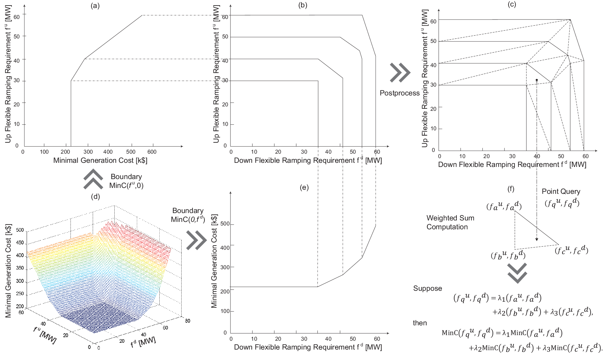
Note that the MinC function is piecewise linear in both arguments. Therefore, it comprises several facets. The general idea to construct the MinC function is to efficiently identify the breaking lines between different facets (i.e., the boundaries of the facets). The horizontal section of a fixed is MaxUR() function. As increases, the number of segments in the MaxUR() function may change. Any such change corresponds to an emerging facet, or a vanishing one. Such changes will also be reflected on the boundaries, specifically, MinC() and MinC(), as breaking points on one or both boundaries. Note that, the breaking points are given by Algorithm 1. Therefore, it suffices to track all the breaking points on both boundaries to identify the breaking lines between different facets.
Algorithm 2: MinC Construction for Computation
Preprocess:
Construct the boundaries: MinC(), and MinC() (Algorithm 1). Denote the breaking points in MinC() by , and the corresponding costs by . Denote the breaking points in MinC() by , and the corresponding costs by .
Main Algorithm:
Postprocess:
Now we obtain the horizonal sections where there is either an emerging facet or a vanishing one. According to the convex property of the MinC function, we can connect the adjacent horizonal sections and partition the feasible region (23)-(25) into triangles, such that there is no breaking line in any of the triangles. Fig. 2 visualizes this algorithm.
The final step returns a set of triangles. For any given parameters , one can query which triangle it belongs to with a binary search (or more advanced query techniques, see [26] for more details). Then, the value of MinC is given by the weighted sum of the three end points of the triangle. An efficient query is crucial for our subsequent linear search algorithm to solve the risk-limiting economic dispatch problem.
We want to emphasize that the number of triangles is limited. Suppose we have decision variables and inequality constraints. Even in the worst case, instead of having triangles, there will be at most triangles [27]. Theoretically, this is already very efficient since the number is almost linear in the input size. In practice, the MinC function is likely to be partitioned into only dozens of triangles (as shown in the case studies), and hence is very efficient to construct.

Although Algorithm 2 is sufficient for computation, it does not provide an intuitive way to visualize the functions. Therefore, we devise an efficient way to obtain the contour of the MinC function with lines in Algorithm 3:
Algorithm 3: MinC Construction for Visualization
- 1.
Calculate by solving the following problem:
(35) - 2.
To obtain the contour of the MinC function, divide the interval [MinC] into equally incremental sub-intervals to draw the contour with lines. Denote the end points by .
- 3.
The contour line with the same cost is simply a MaxUR (or equivalently, MaxDR) function with fixed cost . We may again refer to Algorithm 1 to construct MaxUR() in the interval [].
Using this routine to construct a MinC function with lines, optimization problems need to be solved, where is the number of line segments of function MaxUR() with fixed . Based on the similar argument in the Algorithm 2 analysis, all the ’s are also almost linear in the input size of the problem.
VI Risk-limiting Energy Dispatch
Bearing the relationship between the generation cost and the ramping capacity requirements in mind, we now seek to understand the other dependency - how the ramping capacity requirements depend on the risk-limiting constraint, i.e., to solve the risk-limiting economic dispatch problem. Towards exploiting this dependency, in this section, we first discuss the renewable energy prediction error model. Then, we introduce the linear search algorithm to obtain the optimal combination of the key parameters for flexible ramping products.
VI-A Renewable Energy Prediction Error Model
We use the Bonneville Power Administration (BPA) predicted and actual wind power data [28] with a temporal resolution of 5 minutes to obtain the prediction error model. For a historic dataset for a wind plant with the maximal capacity of 4,500 MW in BPA, we first note that when the power output is less than 10% of the maximal capacity, the relative prediction error can be extremely large (or even arbitrarily large when the actual power output is zero) while the amount of the prediction error is relatively small, which implies the flexible ramping requirements in this case are not critical. Therefore, we trim these data from the dataset. Then, we divide the trimmed historical data into three groups: 10%-30% of the maximal capacity, 30%-70% of the maximal capacity, and above 70% of the maximal capacity. The (relative) prediction error distributions for these three groups are illustrated in Fig. 3. Since prediction errors need to be compensated by ramping generation, the level of prediction errors determines how much ramping capacity is required.
Consequently, we can compare the three cases in Fig. 3. When the wind power output is between 10%-30% of the capacity, the mean prediction error is 7.8 MW with a standard deviation of 223 MW. The relative prediction error is also quite significant in this case, with a mean value of 0.015 and a standard deviation of 0.27. With the increase of the wind power output (between 30%-70% of the capacity, which is the most common range of power output of a wind plant), the relative prediction error drops significantly (with a standard deviation of only 0.14), but the mean value of prediction error shifts to -70.7 MW and its standard deviation is 300 MW. On windy days, with wind power output of more than 70% of the capacity, since we know the maximal capacity of the wind plant, the prediction seems to perform reasonably well, with a mean value of -77.7 MW and a standard deviation of only 175 MW. Also, thanks to this upper bound, the standard deviation of the relative prediction error is now only 0.05.
VI-B Risk-limiting Energy Dispatch
Assuming prediction error distributions as shown in Fig. 3, we seek to achieve the minimal generation cost that satisfies the risk-limiting constraints. Mathematically, if a confidence level of % is desired, the ISO needs to solve the following optimization problem:
| (36) | ||||
Since we use the actual prediction error distributions, there are no symmetric nor other nice analytical properties. Therefore, we propose a linear search method to obtain the minimal generation cost. In particular, for any given parameters (), instead of solving the OPF problem (14), MinC() can be efficiently obtained by querying the set of triangles returned by Algorithm 2.
To formally describe the linear search algorithm, we first divide the search region (given by the prediction error probability distribution) into intervals, each being of length . Suppose and . Then, we employ two for-loops to enumerate all the possible combinations that satisfies the risk-limiting constraint.
For any given specified by the outer for-loop, the inner for-loop tries to identify the shortest interval , which satisfies the risk-limiting constraint. Suppose is the desired parameter to form the shortest interval. Then, we update with , and conduct the comparison to see if the new combination achieves a lower generation cost. Due to the monotonicity of MinC function, there is no need to query MinC(), for any . Thus, we break the inner for-loop. After that, the outer loop starts again, and sets to be . Based on the monotonicity of the cumulative probability distribution, the inner for-loop search process can directly start from the updated .
Algorithm 4: Linear Search Optimal Combination
This search process will query MinC() at most times, which is linear in the length of the interval. However, we want to emphasize that although the linear search is efficient, its accuracy relies on the selection of . If the problem were convex, we could have implemented binary search to achieve arbitrary accuracy. From another point of view, this is also the evidence for the hardness of the non-convexity.
It is worth noting that, the error distributions might be approximated by Gaussian or other well-studied distributions, which can lead to improved accuracy in the solution of the optimization problem but will lead to errors introduced by the approximation of the probability distributions.
VII Case Study


In this section, we first consider a prototype 3-bus system and Garver’s 6-bus system to highlight the properties of our parametric functional approach. Then, we turn to more realistic scenarios by evaluating the influence of flexible ramping products on the WECC 240-bus system. Both simulation results reveal interesting information on the relationship between the generation cost and the key parameters of flexible ramping products. We hope such information can help ISOs to better evaluate the new products and develop methods to achieve the most cost effective market for the new products.
To better quantify the distortion incurred by the new products, we define the distortion cost function DS() as the difference in generation cost between the optimal economic dispatch with flexible ramping requirements () and the optimal dispatch without flexible ramping requirements, i.e.,
| (37) |
Note that DS function is simply the shifted MinC function. Therefore, it preserves all the analytical properties of MinC function. For the subsequent analysis, we will demonstrate the performance of our approach with DS functions.
VII-A Prototype 3-bus System
| [$/MW] | [MW/5 min] | [MW] | [MW] | |
|---|---|---|---|---|
| 50 | 20 | 90 | 100 | |
| 120 | 30 | 0 | 100 | |
| 80 | 20 | 20 | 20 |
We illustrate Algorithm 2 and Algorithm 3 using a prototype 3-bus system. As shown in Fig. 4(a), there are two generators and at bus 1; the third generator is at bus 2; and bus 3 is a load bus. Table I gives the necessary data for the three generators. We assume ’s are all zero for this prototype 3-bus system. We do not consider the line capacity constraints in this example. Assume the generators are to be dispatched for a forecasted net load of 110 MW at , and 120 MW at . Then, without any flexible ramping requirement, the optimal economic dispatch profile at is (100, 0, 10) MW, while it is (100, 0, 20) MW at .
Note that, such economic dispatch comes with free ramping capacity. To reserve ramping capacities for time , the free up-ramping capacity is 30 MW from , which corresponds to the horizontal segment in the lower envelope of Fig. 4(b). We want to highlight that such horizontal region is precisely the non-interesting region discussed in Section IV. After this free and non-interesting region, the two parameters start distorting the generation output profile compared with the optimum given by DS. Similarly, we can analyze the free down-ramping capacity for : 20 MW from plus 20 MW from , which corresponds to the horizontal segment in the lower envelope of Fig. 4(c). Fig. 4(b) and (c), together with the contour of the DS function shown in Fig. 4(d), illustrate all the properties (piece-wise linearity, monotonicity, and convexity) stated in Theorem 2.
Following Algorithm 3 in Section V-B, to efficiently construct the DS function for visualization, we first identify , which according to Fig. 4(d) is given by DS(50,70). We divide [] into 29 slots to obtain the contour of the DS function with 30 lines. In this example, from the constructed function shown in Fig. 4(d), each contour line consists of at most three segments. Hence, the routine requires solving at most 5 optimization problems to construct each contour line.
To efficiently construct the function for computational purposes, we can follow Algorithm 2 to obtain the set of triangles as shown in Fig. 5. The solid lines are given by the main algorithm in Algorithm 2. Based on these solid lines, and the convexity of MinC function, we can conduct the postprocessing part of the algorithm to obtain all the triangles (the dashed lines). Note that there could be different sets of triangles to partition the space. However, the total numbers of triangles for different sets are the same. The system model has 9 decision variables and 27 constraints. Instead of having triangles, there are altogether 29 triangles. This also confirms that the number of triangles will be almost linear in the input size. In fact, as the system scales up, the number of triangles does not grow linearly in practice in that there are often limited binding constraints.

VII-B Garver’s 6-bus System


| [$/MW] | [MW/5 min] | [MW] | [MW] | |
|---|---|---|---|---|
| 58 | 50 | 0 | 200 | |
| 52 | 20 | 130 | 150 | |
| 54 | 20 | 30 | 40 |
We analyze Garver’s 6-bus system [29] shown in Fig. 6. Table II provides the necessary information for the generators at buses 4, 5, and 6. Again, we assume ’s are all zero for this system. The initial generation outputs are 0, 130, and 30 MW, respectively. The loads are located at buses 1, 2, and 3. At time , the forecasted net loads are 59.5 MW each, while at time , the forecasted net loads are 63 MW each. Fig. 7 shows the contour of the DS function for this case.
Suppose now we want to achieve a 30% renewable energy penetration level, as planned by the CAISO for the year of 2020 [30]. And in this test system, the conventional generators contribute around 200 MW, which implies that the wind plant needs to supply 100 MW on average. Based on the current wind power technology [31], the typical wind plant supplies only 20%-40% of its maximal capacity on average. Therefore, we assume there is a wind plant with a maximal capacity of 500 MW in the system.
Fig. 8 shows the possible distortion costs induced by flexible ramping products for the three cases discussed in Section VI-A (low wind, modest wind, and high wind). We compare our risk-limiting economic dispatch approach with a greedy one. The greedy approach selects the parameters (), which is the shortest interval (or minimal ) to achieve the risk-limiting constraint. Mathematically, () employed by the greedy approach is the solution to the following optimization problem:
| (38) | ||||
As shown in Fig. 8, in all the three cases, both our approach and the greedy approach work reasonably well. Yet, our approach outperforms the greedy approach with respect to distortion cost, particularly for the cases with higher wind power output levels (Fig. 8 (b) and (c)). Numerically, compared to the greedy approach, when the confidence level is greater than 90%, the average savings are 15.6% when the predicted wind power is 110 MW, 21.3% when the predicted wind power is 250 MW, and 51.3% when the predicted wind power is 450 MW. We want to emphasize that such savings do not come with expensive computational efforts due to the piecewise linearity of the DS function as we discussed in Section VI-B.

VII-C WECC System


| Bus | [$/MW] | [MW/5 min] | [MW] | [MW] |
|---|---|---|---|---|
| 1034 | 30 | 349.5 | 1200 | 1400 |
| 1232 | 20 | 315 | 1256 | 1256 |
| 1331 | 45 | 610.5 | 510 | 2438 |
| 2130 | 20 | 126 | 500 | 500 |
| 2637 | 55 | 27 | 30 | 110 |
| 4031 | 50 | 244.5 | 220 | 978 |
| 4035 | 20 | 918 | 3671 | 3671 |
| 4039 | 40 | 730.5 | 1000 | 2918 |
| 4131 | 20 | 3240 | 12963 | 12963 |
| 4132 | 30 | 1422 | 4000 | 5693 |
| 4231 | 20 | 904.5 | 3615 | 3615 |
| 4232 | 60 | 142.5 | 150 | 573 |
| 5031 | 30 | 2200.5 | 4000 | 8798.8 |
| 5032 | 20 | 1102.5 | 4410.2 | 4410.5 |
| 6132 | 65 | 535.5 | 550 | 2144 |
| 6235 | 40 | 172.5 | 300 | 693 |
| 6335 | 40 | 202.5 | 600 | 812 |
| 6533 | 80 | 10.5 | 12 | 39 |
| 7032 | 30 | 172.5 | 500 | 691 |
| 8033 | 20 | 393 | 1572 | 1572 |
| 8034 | 70 | 172.5 | 180 | 688 |
Since CAISO is pioneering the design of flexible ramping products, we conduct the same analysis on the WECC 240-bus CAISO model [32]. Table III only provides the information for the generators with ramping capacities11 1 The minimal generation ’s are provided in the model [32].. Note that, to cope with the increasing renewable energy penetration level, we have tripled the ramping capacities in the system. All the other information are the same as suggested by the model.
The initial energy dispatch is determined by a sample load profile. The total load of the sample profile is 180.15 GW. At time and , the forecasted total loads are both 181.15 GW by scaling up the sample load profile. Fig. 9 shows the contour of the DS function for this system.
Based on the same goal of renewable energy penetration level, we assume there is a wind plant with a maximal capacity of 80 GW in the system. Fig. 10 shows the possible distortion costs induced by flexible ramping products for three cases - low wind (16 GW output), modest wind (35 GW output), and high wind (70 GW output). Again, we compare our risk-limiting economic dispatch approach with the greedy approach. As illustrated by Fig. 10, our approach performs much better than the greedy approach even when the confidence level is only 80%. This is because the DS function for this system is even more asymmetric than that for Garver’s 6-bus system (see Fig. 7). The asymmetry results in identifying inefficient up and down ramping capacities. As the feasible region shrinks, the greedy approach finally starts getting better. This again highlights that our approach is very promising, since the greedy algorithm does not have any performance guarantee. Numerically, compared with the greedy approach, when the confidence level is greater than 90%, the average savings are 65.9% when the predicted wind power is 16 GW, 55.5% when the predicted wind power is 35 GW, and 56% when the predicted wind power is 70 GW.
VII-D Extensions
We would like to close this section by briefly discussing the extension of our approach by selecting . To avoid too many arguments, i.e., ’s and ’s, we require the ramping parameters are identical for all time slots, i.e., , and . Fig. 11 shows the contour of the DS function for the WECC system when in this simplified setting.
Comparing Fig. 9 and Fig. 11, we may conclude that although the feasible region for (Fig. 11) is smaller than that for (Fig. 9), considering more time slots exploits more constraints in the system - most of the contour lines in Fig. 11 have one more segment than the corresponding lines in Fig. 9. Hence, the extension suggests our proposed approach to be even more promising.

VIII Conclusions and Future Work
This paper proposes a parametric functional analysis of the relations between the generation cost and the key parameters of the flexible ramping products. We present a novel routine to efficiently construct the introduced functions. Such a routine further yields the efficient risk-limiting economic dispatch. Theoretical analysis exhibits valuable information about such relations whereas simulation results further illustrate how such an approach can be used in practice.
This paper can be extended in various directions. For instance, we have not fully investigated the relationship between the distortion cost and the total capacity payment. Also, it is important to analyze the firm behaviors in the electricity markets with the new products: is it easy to gain market power in such a model? A more accurate empirical evaluation should also include the impacts of existing products, such as frequency regulation, spinning reserves, and non-spinning reserves. Incorporating these existing products will further shrink the feasible region of the MinC function (or equivalently, the DS function), and hence suggest our proposed approach to be even more promising. It is worth noting that our approach is capable of capturing the bidding information for flexible ramping products. Thus, after the bidding structure becomes available in the energy markets, a new empirical evaluation of our approach will be very valuable.
In addition, although we have considered the simple generalization to the case when in Section VII-D, the generalization to a more complicated setting, where all the arguments are allowed to be different, is also very interesting and yet more challenging. Odds are that such generalization may exploit more information on how the dynamics of the renewables affect the electricity market.
Acknowledgement
This research was supported in part by Pennsylvania Infrastructure Technology Alliance and Carnegie Mellon University Scott Institute.
References
- [1] NERC, “Potential reliability impacts of emerging flexible resources,” Special Report, aug 2010.
- [2] E. Lannoye, M. Milligan, J. Adams, A. Tuohy, H. Chandler, D. Flynn, and M. O’Malley, “Integration of variable generation: capacity value and evaluation of flexibility,” in Proc. of IEEE PES General Meeting, 2010.
- [3] K. H. Abdul-Rahman, H. Alarian, M. Rothleder, P. Ristanovic, B. Vesovic, and B. Lu, “Enhanced system reliability using flexible ramp constraint in caiso market,” in Proc. of IEEE PES General Meeting, 2012.
- [4] N. Navid and G. Rosenwald, “Market solutions for managing ramp flexibility with high penetration of renewable resource,” IEEE Trans. on Sustainable Energy, vol. 3, no. 4, pp. 784–790, 2012.
- [5] A. Bergen and V. Vittal, Power systems analysis. Prentice Hall, 1999.
- [6] R. Billinton, Power system reliability evaluation. Taylor & Francis, 1970.
- [7] A. Holder, Parametirc LP Analysis. John Wiley & Sons, 2010.
- [8] K. d. Almeida, F. Galiana, and S. Soares, “A general parametric optimal power flow,” IEEE Trans. on Power Systems, vol. 9, no. 1, pp. 540–547, 1994.
- [9] S. Bose, C. Wu, Y. Xu, A. Wierman, and H. Mohsenian-Rad, “A unifying market power measure for deregulated transmission-constrained electricity markets,” accepted by IEEE Trans. on Power Systems, 2015.
- [10] B. Wang and B. F. Hobbs, “A flexible ramping product: Can it help real-time dispatch markets approach the stochastic dispatch ideal?” Electric Power Systems Research, vol. 109, pp. 128–140, 2014.
- [11] J. A. Taylor, A. Nayyar, D. S. Callaway, and K. Poolla, “Dynamic pricing in consolidated ancillary service markets,” in Proc. of IEEE European Control Conference, 2013, pp. 3032–3037.
- [12] P. Varaiya, F. Wu, and J. Bialek, “Smart operation of smart grid: Risk-limiting dispatch,” Proceedings of the IEEE, pp. 40–57, Jan 2011.
- [13] R. Rajagopal, E. Bitar, P. Varaiya, and F. Wu, “Risk-limiting dispatch for integrating renewable power,” International Journal of Electrical Power & Energy Systems, vol. 44, no. 1, pp. 615 – 628, 2013.
- [14] Y. Zhang, N. Gatsis, and G. Giannakis, “Risk-constrained energy management with multiple wind farms,” in Proc. of IEEE PES ISGT 2013, Feb 2013, pp. 1–6.
- [15] W. Katzenstein and J. Apt, “The cost of wind power variability,” Energy Policy, vol. 51, pp. 233–243, 2012.
- [16] C. Lueken, G. E. Cohen, and J. Apt, “Costs of solar and wind power variability for reducing co2 emissions,” Environmental science & technology, vol. 46, no. 17, pp. 9761–9767, 2012.
- [17] C. Wu, G. Hug, and S. Kar, “A functional approach to assessing flexible ramping products’ impact on electricity market,” Proc. of IEEE ISGT, Feb 2015.
- [18] E. F. Camacho and C. B. Alba, Model predictive control. Springer Science & Business Media, 2013.
- [19] A. Monticelli, M. Pereira, and S. Granville, “Security-constrained optimal power flow with post-contingency corrective rescheduling,” Power Systems, IEEE Transactions on, vol. 2, no. 1, pp. 175–180, 1987.
- [20] F. E. R. Commission et al., “Frequency regulation compensation in the organized wholesale power markets,” Order No. 755-A, pp. 1–76, 2011.
- [21] K. Purchala, L. Meeus, D. Van Dommelen, and R. Belmans, “Usefulness of dc power flow for active power flow analysis,” in Proc. of IEEE PES General Meeting, 2005, pp. 454–459.
- [22] S. P. Boyd and L. Vandenberghe, Convex optimization. Cambridge university press, 2004.
- [23] C. Wu, S. Bose, A. Wierman, and H. Mohesenian-Rad, “A unifying approach to assessing market power in deregulated electricity markets,” in Proc. of IEEE PES General Meeting, 2013.
- [24] CVX Research, Inc., “CVX: Matlab software for disciplined convex programming, version 2.0,” Aug. 2012. [Online]. Available: http://cvxr.com/cvx
- [25] M. Grant and S. Boyd, “Graph implementations for nonsmooth convex programs,” in Recent Advances in Learning and Control, ser. Lecture Notes in Control and Information Sciences, V. Blondel, S. Boyd, and H. Kimura, Eds. Springer-Verlag Limited, 2008, pp. 95–110.
- [26] S. Fortune, “A sweepline algorithm for voronoi diagrams,” Algorithmica, vol. 2, no. 1-4, pp. 153–174, 1987.
- [27] T. K. Dey, “Improved bounds on planar k-sets and k-levels,” in Proc. of 38th Annual Symposium on Foundations of Computer Science. IEEE, 1997, pp. 156–161.
- [28] Bonneville Power Administration, “Wind generation & total load in the bonneville power administration balancing authority,” http://transmission.bpa.gov/Business/operations/Wind.
- [29] L. Garver, “Transmission network estimation using linear programming,” IEEE Trans. on Power Apparatus and Systems, vol. PAS-89, no. 7, pp. 1688–1697, Sept 1970.
- [30] M. Peevey, T. A. Simon, M. P. Florio, C. Sandoval, and M. Ferron, “Decision setting procurement quantity requirements for retail sellers for the renewables portfolio standard program,” Decision 11-12-020, 2011.
- [31] N. Boccard, “Capacity factor of wind power realized values vs. estimates,” energy policy, vol. 37, no. 7, pp. 2679–2688, 2009.
- [32] N.-P. Yu, C.-C. Liu, and J. Price, “Evaluation of market rules using a multi-agent system method,” IEEE Trans. on Power Systems, vol. 25, no. 1, pp. 470–479, Feb 2010.
-A Proof of Theorem 2
We only prove Part (a) as the proofs for Part (b) and (c) are similar. The continuity and piecewise linearity properties of the DS function are a direct result from [7, Theorem 1.1-1.3]. Therefore, we only prove the convexity and monotonicity. Take as an example example and fix .
To prove convexity, consider two arbitrary points
Let , and denote the optimal solution when solving the optimization problem corresponding to DS(). Similarly, let , and denote the optimal solution when solving the optimization problem corresponding to DS(). For any where , we can show that
| (39) | |||
| (40) | |||
| (41) |
construct a feasible (but not necessarily optimal) solution to the optimization problem corresponding to MinC(). Therefore, we have
| (42) | ||||
From (42), for each given , the corresponding MinC function is a convex function [22, Section 3.1.1].
Next, we show that the MinC function is monotonic increasing in the feasible region (23)-(25) by contradiction.
Suppose the minimum of MinC function is achieved at such that . Since the MinC function is continuous, based on the intermediate value theorem, there exists such that , which contradicts the definition of . From this, and since MinC function is convex, it is monotonic increasing over the range in (23)-(25).
-B Proof of Theorem 3
Again, we only show the proof for Part (a) since the remaining part is similar. By the definitions of MinC and MaxUR functions in (37) and (16), for any given , we have
| (43) |
| (44) |
Since the MinC and MaxUR functions are both increasing for given , their inverses are also increasing. As a result, taking MinC at both sides of inequality (43) leads to
| (45) |
Similarly, taking MaxUR-1 at both sides of (44) yields
| (46) |
By selecting , inequality (46) becomes
| (47) |
Using the monotonicity property again, we know
| (48) |
Together, from (45) and (48), we can conclude that
| (49) |
We can show in the same way. This concludes the proof.