跳到论文正文
W Papers独立论文阅读器 arXiv:1409.5146 论文正文 计算阅读时间 · 0%
引用这篇论文根据当前论文元数据生成,正式投稿前建议核对。


License: arXiv.org perpetual non-exclusive license
arXiv:1409.5146v1 [math.CO] 17 Sep 2014

The spectral excess theorem for distance-regular graphs having distance-dd graph with fewer distinct eigenvalues

M.A. Fiol Affiliation: Universitat Politècnica de Catalunya, BarcelonaTechDept. de Matemàtica Aplicada IV, Barcelona, Catalonia(e-mail: fiol@ma4.upc.edu)
Abstract

Let Γ\Gamma be a distance-regular graph with diameter dd and Kneser graph K=ΓdK=\Gamma_{d}, the distance-dd graph of Γ\Gamma. We say that Γ\Gamma is partially antipodal when KK has fewer distinct eigenvalues than Γ\Gamma. In particular, this is the case of antipodal distance-regular graphs (KK with only two distinct eigenvalues), and the so-called half-antipodal distance-regular graphs (KK with only one negative eigenvalue). We provide a characterization of partially antipodal distance-regular graphs (among regular graphs with dd distinct eigenvalues) in terms of the spectrum and the mean number of vertices at maximal distance dd from every vertex. This can be seen as a general version of the so-called spectral excess theorem, which allows us to characterize those distance-regular graphs which are half-antipodal, antipodal, bipartite, or with Kneser graph being strongly regular.

Keywords: Distance-regular graph; Kneser graph; Partial antipodality; Spectrum; Predistance polynomials.

AMS subject classifications: 05C50, 05E30.

1 Preliminaries

Let Γ\Gamma be a distance-regular graph with adjacency matrix AA and d+1d+1 distinct eigenvalues. In the recent work of Brouwer and the author [2], we studied the situation where the distance-dd graph Γd\Gamma_{d} of Γ\Gamma, or Kneser graph KK, with adjacency matrix Ad=pd​(A)A_{d}=p_{d}(A), has fewer distinct eigenvalues. In this case we say that Γ\Gamma is partially antipodal. Examples are the so-called half antipodal (KK with only one negative eigenvalue, up to multiplicity), and antipodal distance-regular graphs (KK being disjoint copies of a complete graph). Here we generalize such a study to the case when Γ\Gamma is a regular graph with d+1d+1 distinct eigenvalues. The main result of this paper is a characterization of partially antipodal distance-regular graphs, among regular graphs with d+1d+1 distinct eigenvalues, in terms of the spectrum and the mean number of vertices at maximal distance dd from every vertex. This can be seen as a general version of the so-called spectral excess theorem, and allows us to characterize those distance-regular graphs which are half antipodal, antipodal, bipartite, or with Kneser graph being strongly regular. Other related characterizations of some of these cases were given by the author in [8, 9, 10]. For background on distance-regular graphs and strongly regular graphs, we refer the reader to Brouwer, Cohen, and Neumaier [1], Brouwer and Haemers [3], and Van Damm, Koolen and Tanaka [6].

Let Γ\Gamma be a regular (connected) graph with degree kk, nn vertices, and spectrum sp⁡Γ={λ0m0,λ1m1,…,λdmd}\spec\Gamma=\{\lambda_{0}^{m_{0}},\lambda_{1}^{m_{1}},\ldots,\lambda_{d}^{m_{d}}\}, where λ0(=k)>λ1>⋯>λd\lambda_{0}(=k)>\lambda_{1}>\cdots>\lambda_{d}, and m0=1m_{0}=1. In this work, we use the following scalar product on the (d+1)(d+1)-dimensional vector space of real polynomials modulo m⁡(x)=∏i=0d(x−λi)m(x)=\prod_{i=0}^{d}(x-\lambda_{i}), that is, the minimal polynomial of AA.

⟨p,q⟩Γ=1n​tr⁡(p⁡(A)​q​(A))=1n​∑i=0dmi​p​(λi)​q​(λi),p,q∈ℝd​[x]/(m⁡(x)).\langle p,q\rangle_{\Gamma}=\frac{1}{n}\tr(p(A)q(A))=\frac{1}{n}\sum_{i=0}^{d}m_{i}p(\lambda_{i})q(\lambda_{i}),\qquad p,q\in\mathbb{R}_{d}[x]/(m(x)). (1)

This is a special case of the inner product of symmetric n×nn\times n real matrices M,NM,N, defined by ⟨M,N⟩=1n​tr⁡(M​N)\langle M,N\rangle=\frac{1}{n}\tr(MN). The predistance polynomials p0,p1,…,pdp_{0},p_{1},\ldots,p_{d}, introduced by the author and Garriga [13], are a sequence of orthogonal polynomials with respect to the inner product (1), normalized in such a way that ‖pi‖Γ2=pi​(k)\|p_{i}\|^{2}_{\Gamma}=p_{i}(k). Then, it is known that Γ\Gamma is distance-regular if and only if such polynomials satisfy pi​(A)=Aip_{i}(A)=A_{i} (the adjacency matrix of the distance-ii graph Γi\Gamma_{i}) for i=0,…,di=0,\ldots,d, in which case they turn out to be the distance polynomials. In fact, we have the following strongest proposition, which is a combination of results in [14, 7].

Proposition 1.

A regular graph Γ\Gamma as above is distance-regular if and only if there exists a polynomial pp of degree dd such that p⁡(A)=Adp(A)=A_{d}, in which case p=pdp=p_{d}. □\Box

Moreover, the Hoffman polynomial HH, such that H⁡(λi)=n​δ0​iH(\lambda_{i})=n\delta_{0i} and H⁡(A)=JH(A)=J, turns out to be H=p0+p1+⋯+pdH=p_{0}+p_{1}+\cdots+p_{d}. Also, as in the case of distance-regular graphs, the multiplicities of Γ\Gamma can be obtained from the values of pdp_{d} since,

(−1)ipd(λi)πimi=pd(λ0)π0,i=1,…,d.(-1)^{i}p_{d}(\lambda_{i})\pi_{i}m_{i}=p_{d}(\lambda_{0})\pi_{0},\qquad i=1,\ldots,d. (2)

where πi=∏j≠i|λi−λj|\pi_{i}=\prod_{j\neq i}|\lambda_{i}-\lambda_{j}|. Indeed, let Li​(x)=∏j≠0,i(x−λj)/∏j≠0,i(λi−λj)L_{i}(x)=\prod_{j\neq 0,i}(x-\lambda_{j})/\prod_{j\neq 0,i}(\lambda_{i}-\lambda_{j}). Then, since dgr⁡Li=d−1\dgr L_{i}=d-1, (2) follows from ⟨Li,pd⟩Γ=0\langle L_{i},p_{d}\rangle_{\Gamma}=0 for i=1,…,di=1,\ldots,d. Some interesting consequences of the above, together with other properties of the predistance polynomials are the following (for more details, see [4]):

  • •

    The values of pdp_{d} at λ0,λ1,…,λd\lambda_{0},\lambda_{1},\ldots,\lambda_{d} alternate in sign.

  • •

    Using the values of pd​(λi)p_{d}(\lambda_{i}), i=0,…,di=0,\ldots,d, given by (2), in the equality ‖pd‖Γ2=pd​(λ0)\|p_{d}\|_{\Gamma}^{2}=p_{d}(\lambda_{0}), and solving for pd​(λ0)p_{d}(\lambda_{0}) we get the so-called spectral excess

    pd​(λ0)=n​(π02mi​pi2)−1.p_{d}(\lambda_{0})=n\left(\frac{\pi_{0}^{2}}{m_{i}p_{i}^{2}}\right)^{-1}. (3)
  • •

    For every i=0,…,di=0,\ldots,d, (any multiple of) the sum polynomial qi=p0+⋯+piq_{i}=p_{0}+\cdots+p_{i} maximizes the quotient r⁡(λ0)/‖r‖Γr(\lambda_{0})/\|r\|_{\Gamma} among the polynomials r∈ℝi​[x]r\in\mathbb{R}_{i}[x] (notice that qi​(λ0)2/‖qi‖Γ2=qi​(λ0CLOSEq_{i}(\lambda_{0})^{2}/\|q_{i}\|_{\Gamma}^{2}=q_{i}(\lambda_{0})), and (1=)q0(λ0)<q1(λ0)<⋯<qd(λ0)(=H(λ0)=n)(1=)q_{0}(\lambda_{0})<q_{1}(\lambda_{0})<\cdots<q_{d}(\lambda_{0})(=H(\lambda_{0})=n).

Let Γ\Gamma have nn vertices, d+1d+1 distinct eigenvalues, and diameter D(≤d)D(\leq d). For i=0,…,Di=0,\ldots,D, let ki​(u)k_{i}(u) be the number of vertices at distance ii from vertex uu. Let si​(u)=k0​(u)+⋯+ki​(u)s_{i}(u)=k_{0}(u)+\cdots+k_{i}(u). Of course, s0​(u)=1s_{0}(u)=1 and sD​(u)=ns_{D}(u)=n. The following result can be seen as a version of the spectral excess theorem, due to Garriga and the author [13] (for short proofs, see Van Dam [5], and Fiol, Gago and Garriga [12]):

Theorem 2.

Let Γ\Gamma be a regular graph with spectrum sp⁡Γ={λ0,λ1m1,…,λdmd}\spec\Gamma=\{\lambda_{0},\lambda_{1}^{m_{1}},\ldots,\lambda_{d}^{m_{d}}\}, where λ0>λ1>⋯>λd\lambda_{0}>\lambda_{1}>\cdots>\lambda_{d}. Let si¯=1n​∑u∈Vsi​(u)\overline{s_{i}}=\frac{1}{n}\sum_{u\in V}s_{i}(u) be the average number of vertices at distance at most ii from every vertex in Γ\Gamma. Then, for any polynomial r∈ℝd−1​[x]r\in\mathbb{R}_{d-1}[x] we have

r​(λ0)2‖r‖Γ2≤sd−1¯,\frac{r(\lambda_{0})^{2}}{\|r\|_{\Gamma}^{2}}\leq\overline{s_{d-1}}, (4)

with equality if and only if Γ\Gamma is distance-regular and rr is a nonzero multiple of qd−1q_{d-1}.

Proof.

Let Sd−1=I+A+⋯+Ad−1S_{d-1}=I+A+\cdots+A_{d-1}. As dgr⁡r≤d−1\dgr r\leq d-1, ⟨r⁡(A),J⟩=⟨r⁡(A),Sd−1⟩\langle r(A),J\rangle=\langle r(A),S_{d-1}\rangle. But ⟨r⁡(A),J⟩=⟨r,H⟩Γ=r⁡(λ0)\langle r(A),J\rangle=\langle r,H\rangle_{\Gamma}=r(\lambda_{0}). Thus, Cauchy-Schwarz inequality gives

r2​(λ0)≤‖r⁡(A)‖2​‖Sd−1‖2=‖r‖Γ2​sd−1¯,r^{2}(\lambda_{0})\leq\|r(A)\|^{2}\|S_{d-1}\|^{2}=\|r\|^{2}_{\Gamma}\overline{s_{d-1}},

whence (4) follows. Besides, in case of equality we have that r⁡(A)=α​Sd−1r(A)=\alpha S_{d-1} for some nonzero constant α\alpha. Hence, the polynomial p=H−(1/α)​rp=H-(1/\alpha)r satisfies p⁡(A)=J−Sd−1=Adp(A)=J-S_{d-1}=A_{d} and, from Proposition 1, Γ\Gamma is distance-regular, p=pdp=p_{d}, and r=α​qd−1r=\alpha q_{d-1}. The converse in clear from sd−1=n−kd=H⁡(λ0)−pd​(λ0)=qd−1​(λ0)s_{d-1}=n-k_{d}=H(\lambda_{0})-p_{d}(\lambda_{0})=q_{d-1}(\lambda_{0}). ∎

In fact, as it was shown in [11], the above result still holds if we change the arithmetic mean of the numbers sd−1​(u)s_{d-1}(u), u∈Vu\in V, by its harmonic mean.

2 The results

As commented above, in [2] we studied the situation where the distance-dd graph Γd\Gamma_{d}, of a distance-regular graph Γ\Gamma with diameter dd, has fewer distinct eigenvalues. Now, we are interested in the case when Γ\Gamma is regular and with d+1d+1 distinct eigenvalues. In this context, pdp_{d} is the highest degree predistance polynomial and, as pd​(A)p_{d}(A) is not necessarily the distance-dd matrix AdA_{d} (usually not even a 00-11 matrix), we consider the distinct eigenvalues of pd​(A)p_{d}(A) vs. those of AA. More precisely, given a set H⊂{0,…,d}H\subset\{0,\ldots,d\}, we give conditions for all pd​(λi)p_{d}(\lambda_{i}) with i∈Hi\in H taking the same value. Notice that, because the values of pdp_{d} at the mesh λ0,λ1,…,λd\lambda_{0},\lambda_{1},\ldots,\lambda_{d} alternate in sign, the feasible sets HH must have either even or odd numbers

The case 𝝀𝟎∉𝑯\lambda_{0}\notin H

We first study the more common case when λ0∉H\lambda_{0}\notin H. For i=1,…,di=1,\ldots,d, let ϕi​(x)=∏j≠0,i(x−λi)\phi_{i}(x)=\prod_{j\neq 0,i}(x-\lambda_{i}), and consider again the Lagrange interpolating polynomial Li​(x)=ϕi​(x)/ϕ⁡(λi)L_{i}(x)=\phi_{i}(x)/\phi(\lambda_{i}), satisfying Li​(λj)=δi​jL_{i}(\lambda_{j})=\delta_{ij} for j≠0j\neq 0, and Li​(λ0)=(−1)i+1​π0πiL_{i}(\lambda_{0})=(-1)^{i+1}\frac{\pi_{0}}{\pi_{i}}, where πi=|ϕi​(λi)|\pi_{i}=|\phi_{i}(\lambda_{i})|.

Theorem 3.

Let Γ\Gamma be a regular graph with degree kk, nn vertices, and spectrum sp⁡Γ={λ0,λ1m1,…,λdmd}\spec\Gamma=\{\lambda_{0},\lambda_{1}^{m_{1}},\ldots,\lambda_{d}^{m_{d}}\}, where λ0(=k)>λ1>⋯>λd\lambda_{0}(=k)>\lambda_{1}>\cdots>\lambda_{d}. Let H⊂{1,…,d}H\subset\{1,\ldots,d\}. For every i=0,…,di=0,\ldots,d, let πi=∏j≠i|λi−λj|\pi_{i}=\prod_{j\neq i}|\lambda_{i}-\lambda_{j}|. Let kd¯=1n​∑u∈Vkd​(u)\overline{k_{d}}=\frac{1}{n}\sum_{u\in V}k_{d}(u) be the average number of vertices at distance dd from every vertex in Γ\Gamma. Then,

kd¯≤n​∑i∈Hmi(∑i∈Hπ0πi)2+∑i∉Hπ02mi​πi2​∑i∈Hmi,\overline{k_{d}}\leq\frac{n\sum_{i\in H}m_{i}}{\left(\sum_{i\in H}\frac{\pi_{0}}{\pi_{i}}\right)^{2}+\sum_{i\notin H}\frac{\pi_{0}^{2}}{m_{i}\pi_{i}^{2}}\sum_{i\in H}m_{i}}, (5)

and equality holds if and only if Γ\Gamma is a distance-regular graph with constant Pi​d=pd​(λi)P_{id}=p_{d}(\lambda_{i}) for every i∈Hi\in H.

Proof.

The clue is to apply Theorem 2 with a polynomial r∈ℝd−1​[x]r\in\mathbb{R}_{d-1}[x] having the desired properties of qd−1q_{d-1}. To this end, first notice that, as qd−1=H−pdq_{d-1}=H-p_{d}, we have qd−1​(λi)=−pd​(λi)q_{d-1}(\lambda_{i})=-p_{d}(\lambda_{i}) for any i≠0i\neq 0. Thus, we take the polynomial rr with values r⁡(λi)=−tr(\lambda_{i})=-t for i∈Hi\in H, and r⁡(λi)=−pd​(λi)r(\lambda_{i})=-p_{d}(\lambda_{i}) for i∉Hi\notin H, i≠0i\neq 0. Then, using (2),

r⁡(x)\displaystyle r(x) =−t∑i∈HLi(x)−∑i∉H,i≠0pd(λi)Li(x),\displaystyle=-t\sum_{i\in H}L_{i}(x)-\sum_{i\notin H,i\neq 0}p_{d}(\lambda_{i})L_{i}(x),
r⁡(λ0)\displaystyle r(\lambda_{0}) =−t∑i∈H(−1)i+1π0πi−∑i∉H,i≠0pd(λi)(−1)i+1π0πi\displaystyle=-t\sum_{i\in H}(-1)^{i+1}\frac{\pi_{0}}{\pi_{i}}-\sum_{i\notin H,i\neq 0}p_{d}(\lambda_{i})(-1)^{i+1}\frac{\pi_{0}}{\pi_{i}}
=−t∑i∈H(−1)i+1π0πi−pd(λ0)2∑i∉H,i≠0π02mi​πi2,\displaystyle=-t\sum_{i\in H}(-1)^{i+1}\frac{\pi_{0}}{\pi_{i}}-p_{d}(\lambda_{0})^{2}\sum_{i\notin H,i\neq 0}\frac{\pi_{0}^{2}}{m_{i}\pi_{i}^{2}},
n​‖r‖Γ2\displaystyle n\|r\|^{2}_{\Gamma} =r​(λ0)2+t2​∑i∈Hmi+∑i∉H,i≠0mi​pd​(λi)2.\displaystyle=r(\lambda_{0})^{2}+t^{2}\sum_{i\in H}m_{i}+\sum_{i\notin H,i\neq 0}m_{i}p_{d}(\lambda_{i})^{2}.

Thus, (4) yields

Φ⁡(t)=r​(λ0)2‖r‖Γ2=n​(α​t+β)2(α​t+β)2+σ​t2+γ≤sd−1¯\Phi(t)=\frac{r(\lambda_{0})^{2}}{\|r\|_{\Gamma}^{2}}=\frac{n(\alpha t+\beta)^{2}}{(\alpha t+\beta)^{2}+\sigma t^{2}+\gamma}\leq\overline{s_{d-1}} (6)

where

α\displaystyle\alpha =∑i∈H(−1)i+1π0πi,β=−pd(λ0)∑i∉H,i≠0π02mi​πi2,\displaystyle=\sum_{i\in H}(-1)^{i+1}\frac{\pi_{0}}{\pi_{i}},\qquad\qquad\qquad\beta=-p_{d}(\lambda_{0})\sum_{i\notin H,i\neq 0}\frac{\pi_{0}^{2}}{m_{i}\pi_{i}^{2}}, (7)
γ\displaystyle\gamma =∑i∉H,i≠0mi​pd​(λi)2=∑i∉H,i≠0pd​(λ0)2mi​π02πi2=−pd​(λ0)​β,σ=∑i∈Hmi.\displaystyle=\sum_{i\notin H,i\neq 0}m_{i}p_{d}(\lambda_{i})^{2}=\sum_{i\notin H,i\neq 0}\frac{p_{d}(\lambda_{0})^{2}}{m_{i}}\frac{\pi_{0}^{2}}{\pi_{i}^{2}}=-p_{d}(\lambda_{0})\beta,\qquad\sigma=\sum_{i\in H}m_{i}. (8)

Now, to have the best result in (6) (and since we are mostly interested in the case of equality), we have to find the maximum of the function Φ⁡(t)\Phi(t), which is attained at t0=α​γ/β​σt_{0}=\alpha\gamma/\beta\sigma. Then,

Φmax=Φ⁡(t0)=n⁡(α2​γ+β2​σ)α2​γ+β2​σ+γ​σ≤sd−1¯=n−kd¯.\Phi_{\max}=\Phi(t_{0})=\frac{n(\alpha^{2}\gamma+\beta^{2}\sigma)}{\alpha^{2}\gamma+\beta^{2}\sigma+\gamma\sigma}\leq\overline{s_{d-1}}=n-\overline{k_{d}}.

Thus, using (7)-(8) and simplifying we get (5). In case of equality, we know, by Theorem 2, that Γ\Gamma is distance-regular with r⁡(x)=α​qd−1​(x)r(x)=\alpha q_{d-1}(x) for some constant α\alpha. If i∉H,i≠0i\notin H,i\neq 0, r⁡(λi)=−pd​(λi)=α​qd−1​(λi)=−α​pd​(λi)r(\lambda_{i})=-p_{d}(\lambda_{i})=\alpha q_{d-1}(\lambda_{i})=-\alpha p_{d}(\lambda_{i}), so that α=1\alpha=1 since pd​(λi)≠0p_{d}(\lambda_{i})\neq 0. Then, for every i∈Hi\in H, we get

Pi​d=pd​(λi)=H⁡(λi)−qd−1​(λi)=−r⁡(λi)=t0.P_{id}=p_{d}(\lambda_{i})=H(\lambda_{i})-q_{d-1}(\lambda_{i})=-r(\lambda_{i})=t_{0}.

Conversely, if Γ\Gamma is distance-regular, we have that kd¯=kd\overline{k_{d}}=k_{d}, and, if Pi​dP_{id} is a constant, say, τ\tau for every i∈Hi\in H, we obtain, from (2), that σ=kdpd​(λi)​∑i∈H(−1)i​π0πi=kdτ​α\sigma=\frac{k_{d}}{p_{d}(\lambda_{i})}\sum_{i\in H}(-1)^{i}\frac{\pi_{0}}{\pi_{i}}=\frac{k_{d}}{\tau}\alpha, whence τ=1σ​kd​α\tau=\frac{1}{\sigma}k_{d}\alpha. Moreover,

n​kd=‖pd‖Γ2=∑i∉Hmi​pd​(λi)2+∑i∈Hmi​τ2=kd2​∑i∉Hπ02mi​πi2+kd2​(∑i∈Hπ0πi)2∑i∈Hmi,nk_{d}=\|p_{d}\|_{\Gamma}^{2}=\sum_{i\notin H}m_{i}p_{d}(\lambda_{i})^{2}+\sum_{i\in H}m_{i}\tau^{2}=k_{d}^{2}\sum_{i\notin H}\frac{\pi_{0}^{2}}{m_{i}\pi_{i}^{2}}+k_{d}^{2}\frac{\left(\sum_{i\in H}\frac{\pi_{0}}{\pi_{i}}\right)^{2}}{\sum_{i\in H}m_{i}},

and equality in (10) holds. ∎

As mentioned above, when Γ\Gamma is already a distance-regular graph, Brouwer and the author [2] gave parameter conditions for partial antipodality, and surveyed known examples. The different examples given here are withdrawn from such a paper.

Example 4.

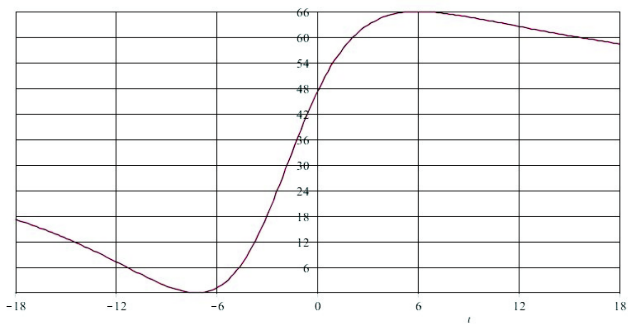
The Odd graph O5O_{5}, on n=126n=126 vertices, has intersection array {5,4,4,3;1,1,2,2}\{5,4,4,3;1,1,2,2\}, so that kd=60k_{d}=60, and spectrum 51,327,142,−248,−485^{1},3^{27},1^{42},-2^{48},-4^{8}. Then, with H={2,4}H=\{2,4\}, the function Φ⁡(t)\Phi(t) is depicted in Fig. 1. Its maximum is attained for t0=6t_{0}=6, and its value is Φ⁡(6)=66=sd−1\Phi(6)=66=s_{d-1}. Then, P24=P44P_{24}=P_{44}.

Refer to caption
Figure 1: The function Φ⁡(t)\Phi(t) for O5O_{5} with H={2,4}H=\{2,4\}.

Notice that if, in the above result, HH is a singleton, there is no restriction for the values of pdp_{d}, and then we get the so-called spectral excess theorem (originally proved by Garriga and the author [13]).

Corollary 5 (The spectral excess theorem).

Let Γ\Gamma be a regular graph with spectrum sp⁡Γ\spec\Gamma and average number kd¯\overline{k_{d}} as above. Then Γ\Gamma is distance-regular if and only if

kd¯=pd​(λ0)=n​(∑i=0dπ02mi​πi2)−1.\overline{k_{d}}=p_{d}(\lambda_{0})=n\left(\sum_{i=0}^{d}\frac{\pi_{0}^{2}}{m_{i}\pi_{i}^{2}}\right)^{-1}.
Proof.

Take H={i}H=\{i\} for some i≠0i\neq 0 in Theorem 3. ∎

As mentioned before, in [2] a distance-regular graph Γ\Gamma was said to be half antipodal if the distance-dd graph has only one negative eigenvalue (i.e., Pi​dP_{id} is a constant for every i=1,3,…i=1,3,\ldots). Then, a direct consequence of Theorem 3 by taking H=Hodd={1,3,…}H=H_{\mbox{\scriptsize odd}}=\{1,3,\ldots\} is the following characterization of half antipodality.

Corollary 6.

Let Γ\Gamma be a regular graph as above. Then,

kd¯≤n​∑i oddmi(∑i oddπ0πi)2+∑i evenπ02mi​πi2​∑i oddmi,\overline{k_{d}}\leq\frac{n\sum_{\mbox{\scriptsize$i$ odd}}m_{i}}{\left(\sum_{\mbox{\scriptsize$i$ odd}}\frac{\pi_{0}}{\pi_{i}}\right)^{2}+\sum_{\mbox{\scriptsize$i$ even}}\frac{\pi_{0}^{2}}{m_{i}\pi_{i}^{2}}\sum_{\mbox{\scriptsize$i$ odd}}m_{i}}, (9)

and equality holds if and only if Γ\Gamma is a half antipodal distance-regular graph. □\Box

Recall that a regular graph is strongly regular if and only if it has at most three distinct eigenvalues (see e.g. [15]). Then, we can apply Theorem 3 with Heven={2,4,…}H_{\mbox{\scriptsize even}}=\{2,4,\ldots\} and Hodd={1,3,…}H_{\mbox{\scriptsize odd}}=\{1,3,\ldots\} (and add up the two inequalities obtained) to obtain a characterization of those distance-regular graphs having strongly regular distance-dd graph.

Corollary 7.

Let Γ\Gamma be a regular graph as above. Then,

kd¯≤n2(∑i evenπ0πi)2+(∑i oddπ0πi)2+∑i evenπ02mi​πi2​∑i oddmi+∑i oddπ02mi​πi2​∑i evenmi,\overline{k_{d}}\leq\frac{n^{2}}{\displaystyle\left(\sum_{\mbox{\scriptsize$i$ even}}\frac{\pi_{0}}{\pi_{i}}\right)^{2}+\left(\sum_{\mbox{\scriptsize$i$ odd}}\frac{\pi_{0}}{\pi_{i}}\right)^{2}+\sum_{\mbox{\scriptsize$i$ even}}\frac{\pi_{0}^{2}}{m_{i}\pi_{i}^{2}}\sum_{\mbox{\scriptsize$i$ odd}}m_{i}+\sum_{\mbox{\scriptsize$i$ odd}}\frac{\pi_{0}^{2}}{m_{i}\pi_{i}^{2}}\sum_{\mbox{\scriptsize$i$ even}}m_{i}}, (10)

and equality holds if and only if Γ\Gamma is a distance-regular graph with strongly regular distance-dd graph Γd\Gamma_{d}. □\Box

Example 8.

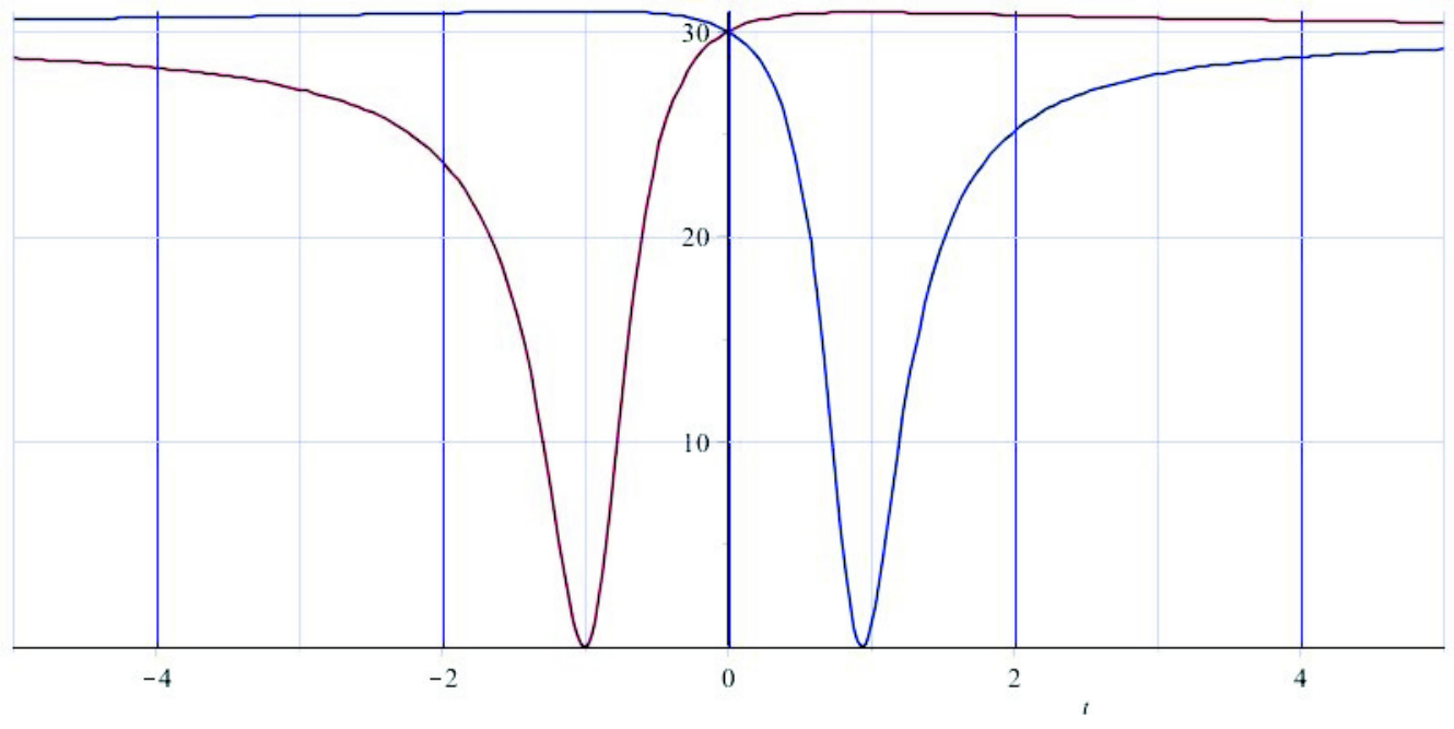
The Wells graph, on n=32n=32 vertices, has intersection array {5,4,1,1;1,1,4,5}\{5,4,1,1;1,1,4,5\} and spectrum 51,58,110,−58,−355^{1},\sqrt{5}^{8},1^{10},-\sqrt{5}^{8},-3^{5}. This graph is 22-antipodal, so that kd=1k_{d}=1. Then, Fig. 2 shows the functions Φ0​(t)\Phi_{0}(t) with H0={2,4}H_{0}=\{2,4\}, and Φ1​(t)\Phi_{1}(t) with H1={1,3}H_{1}=\{1,3\}. Their (common) maximum value is attained for t0=1t_{0}=1 and t1=−1t_{1}=-1, respectively, and it is Φ0​(1)=Φ1​(−1)=31=sd−1\Phi_{0}(1)=\Phi_{1}(-1)=31=s_{d-1}. Then, P24=P44P_{24}=P_{44} and P14=P34P_{14}=P_{34}.

Refer to caption
Figure 2: The functions Φ0​(t)\Phi_{0}(t) (in red) with H0={2,4}H_{0}=\{2,4\}, and Φ1​(t)\Phi_{1}(t) (in blue) with H1={1,3}H_{1}=\{1,3\} of the Wells graph.

In fact, the above expression can be simplified because ∑i evenmi+∑i oddmi=n\sum_{\mbox{\scriptsize$i$ even}}m_{i}+\sum_{\mbox{\scriptsize$i$ odd}}m_{i}=n, ∑i evenπ0πi=∑i oddπ0πi\sum_{\mbox{\scriptsize$i$ even}}\frac{\pi_{0}}{\pi_{i}}=\sum_{\mbox{\scriptsize$i$ odd}}\frac{\pi_{0}}{\pi_{i}} (see [9]), and, from (3), ∑i evenπ02mi​πi2+∑i oddπ02mi​πi2=n/pd​(λ0)\sum_{\mbox{\scriptsize$i$ even}}\frac{\pi_{0}^{2}}{m_{i}\pi_{i}^{2}}+\sum_{\mbox{\scriptsize$i$ odd}}\frac{\pi_{0}^{2}}{m_{i}\pi_{i}^{2}}=n/p_{d}(\lambda_{0}). Anyway, we have written (10) as it is to emphasize the ‘symmetries’ between even and odd terms.

The following result was used in [2, 10] for the case of distance-regular graphs (where pd​(λi)=Pi​dp_{d}(\lambda_{i})=P_{id}).

Corollary 9.

Let Γ\Gamma be a regular graph with eigenvalues λ0>λ1>⋯>λd\lambda_{0}>\lambda_{1}>\cdots>\lambda_{d}. Let H⊂{1,…,d}H\subset\{1,\ldots,d\}. Then, pd​(λi)=pd​(λj)p_{d}(\lambda_{i})=p_{d}(\lambda_{j}) for every i,j∈Hi,j\in H if and only if ∑i≠j(mi​πi−mj​πj)2=0\sum_{i\neq j}(m_{i}\pi_{i}-m_{j}\pi_{j})^{2}=0.

Proof.

Notice that the right hand side of (5) is just the spectral excess pd​(λ0)p_{d}(\lambda_{0}), which is given by (3). Then, the result follows from from equating both expressions and simplifying. ∎

The case 𝝀𝟎∈𝑯\lambda_{0}\in H

To deal with this case, we could proceed as above by defining conveniently a degree d−1d-1 polynomial rr. Then the proof is similar to the one for Theorem 3. If λ0∈H\lambda_{0}\in H then p⁡(λi)=p⁡(λ0)p(\lambda_{i})=p(\lambda_{0}) for any i∈Hi\in H. Moreover, the odd indexes, cannot belong to HH. In particular 1∉H1\notin H. For instance, a possible choice for r∈ℝd−1​[x]r\in\mathbb{R}_{d-1}[x] is:

  • •

    r⁡(λ0)=n−pd​(λ0)r(\lambda_{0})=n-p_{d}(\lambda_{0}), r⁡(λi)=−pd​(λ0)r(\lambda_{i})=-p_{d}(\lambda_{0}) for i∈Hi\in H, i≠0i\neq 0.

  • •

    r⁡(λi)=−t​pd​(λi)r(\lambda_{i})=-tp_{d}(\lambda_{i}) for i∉Hi\notin H, i≠1i\neq 1,

Hovewer, we can follow a more direct approach by using (6). First, the following result was proved in [2]:

Proposition 10 ([2, Prop. 8]).

Let Γ\Gamma be a distance regular graph with diameter dd. If P0​d=Pi​dP_{0d}=P_{id} then ii is even. Let i>0i>0 be even. Then P0​d=Pi​dP_{0d}=P_{id} if and only Γ\Gamma is antipodal, or i=di=d and Γ\Gamma is bipartite. □\Box

Theorem 11.

Let Γ\Gamma be a regular graph with nn vertices, spectrum sp⁡Γ\spec\Gamma as above, and mean excess kd¯\overline{k_{d}}. Then, for every i=1,…,di=1,\ldots,d,

kd¯≤n⁡(mi+∑j≠0,iπ02mj​πj2)(π0πi+∑j≠0,iπ02mj​πj2)2+mi+∑j≠0,iπ02mj​πj2.\overline{k_{d}}\leq\frac{n\left(m_{i}+\sum_{j\neq 0,i}\frac{\pi_{0}^{2}}{m_{j}\pi_{j}^{2}}\right)}{\left(\frac{\pi_{0}}{\pi_{i}}+\sum_{j\neq 0,i}\frac{\pi_{0}^{2}}{m_{j}\pi_{j}^{2}}\right)^{2}+m_{i}+\sum_{j\neq 0,i}\frac{\pi_{0}^{2}}{m_{j}\pi_{j}^{2}}}. (11)

Moreover:

  • (a)(a)

    Equality holds for some i≠di\neq d if and only it holds for any i=1,…,di=1,\ldots,d and Γ\Gamma is an antipodal distance-regular graph.

  • (b)(b)

    Equality holds only for i=di=d if and only if Γ\Gamma is a bipartite, but not antipodal, distance-regular graph.

Proof.

The inequality (11) follows from (6) by taking H={i}H=\{i\} for some even i≠0i\neq 0, and choosing t=pd​(λ0)t=p_{d}(\lambda_{0}). Then, in case of equality, Theorem 3 tells us that Γ\Gamma is distance-regular. Then, Γd\Gamma_{d} is a regular graph with equal eigenvalues P0​dP_{0d} and Pi​dP_{id}. So, the result follows from Proposition 10. ∎

Example 12.

For the Wells graph the right hand expression of (11) gives 1(=k4)1(=k_{4}) for any i=1,…,4i=1,\ldots,4, in concordance with its antipodal character. In contrast, the folded 1010-cube F​Q10FQ_{10}, on n=512n=512 vertices, has intersection array {10,9,8,7,6;1,2,3,4,10}\{10,9,8,7,6;1,2,3,4,10\} and spectrum 101,645,2210,−2210,−645,−10110^{1},6^{45},2^{210},-2^{210},-6^{45},-10^{1}. Then, the right hand expression of (11) gives 234.16234.16, 293.36293.36, 293.36293.36, 234.16234.16 for i=1,2,3,4i=1,2,3,4, respectively, and 126(=k5)126(=k_{5}) for i=5i=5, showing that F​Q10FQ_{10} is a bipartite distance-regular graph, but not antipodal.

Another characterization of antipodal distance-regular graphs was given by the author in [8] by assuming that the distance dd-graph of a regular graph is already antipodal.

Acknowledgments

Research supported by the Ministerio de Ciencia e Innovación, Spain, and the European Regional Development Fund under project MTM2011-28800-C02-01.

References

  • [1] A.E. Brouwer, A.M. Cohen, and A. Neumaier, Distance-Regular Graphs, Springer-Verlag, Berlin-New York, 1989.
  • [2] A.E. Brouwer and M.A. Fiol, Distance-regular graphs where the distance-dd graph has fewer distinct eigenvalues, preprint (2014); arXiv:1409.0389 [math.CO].
  • [3] A.E. Brouwer and W.H. Haemers, Spectra of Graphs, Springer, 2012; available online at http://homepages.cwi.nl/~aeb/math/ipm/.
  • [4] M. Cámara, J. Fàbrega, M.A. Fiol, and E. Garriga, Some families of orthogonal polynomials of a discrete variable and their applications to graphs and codes, Electron. J. Combin. 16(1) (2009), #R83.
  • [5] E.R. van Dam, The spectral excess theorem for distance-regular graphs: a global (over)view, Electron. J. Combin. 15(1) (2008), #R129.
  • [6] E.R. van Dam, J.H. Koolen, and H. Tanaka, Distance-regular graphs, manuscript (2014), available online at https://sites.google.com/site/edwinrvandam/home/papers/drg.pdf.
  • [7] C. Dalfó, E.R. van Dam, M.A. Fiol, E. Garriga, and B.L. Gorissen, On almost distance-regular graphs, J. Combin. Theory, Ser. A 118 (2011) 1094–1113.
  • [8] M.A. Fiol, An eigenvalue characterization of antipodal distance-regular graphs, Electron. J. Combin. 4 (1997), #R30.
  • [9] M.A. Fiol, A quasi-spectral characterization of strongly distance-regular graphs, Electron. J. Combin. 7 (2000), #R51.
  • [10] M.A. Fiol, Some spectral characterization of strongly distance-regular graphs, Combin. Probab. Comput. 10 (2001), no. 2, 127–135.
  • [11] M.A. Fiol, Algebraic characterizations of distance-regular graphs, Discrete Math. 246 (2002) 111–129.
  • [12] M.A. Fiol, S. Gago, and E. Garriga, A simple proof of the spectral excess theorem for distance-regular graphs, Linear Algebra Appl. 432 (2010), 2418–2422.
  • [13] M.A. Fiol and E. Garriga, From local adjacency polynomials to locally pseudo-distance-regular graphs, J. Combin. Theory Ser. B 71 (1997), 162–183.
  • [14] M.A. Fiol, E. Garriga, and J.L.A. Yebra, Locally pseudo-distance-regular graphs, J. Combin. Theory Ser. B 68 (1996), 179–205.
  • [15] C.D. Godsil, Algebraic Combinatorics, Chapman and Hall, NewYork, 1993.