Self-similar groups, automatic sequences, and unitriangular representations

R. Grigorchuk Y. Leonov V. Nekrashevych V. Sushchansky

1 Introduction

Self-similar groups is an active topic of modern group theory. They initially appeared as interesting examples of groups with unusual properties (see [Ale72, Sus79, Gri80, GS83]). The main techniques of the theory were developed for the study of these examples. Later a connection to dynamical systems was discovered (see [Nek03, Nek05]) via the notion of the iterated monodromy group. Many interesting problems were solved using self-similar groups (see [Gri98, GLSŻ00, BV05, BN06]).

One of the ways to define self-similar groups is to say that they are groups generated by all states of an automaton (of Mealy type, also called a transducer, or sequential machine). Especially important case is when the group is generated by the states of a finite automaton. All examples mentioned above (including the iterated monodromy groups of expanding dynamical systems) are like that.

The main goal of this article is to indicate a new relation between self-similar groups and another classical notion of automaticity: automatic sequences and matrices. See the monographs [AS03, vH03] for theory of automatic sequences and applications.

More precisely, we are going to study natural linear representations of self-similar groups over finite fields, and show that matrices associated with elements of a group generated by a finite automaton are automatic.

There are several ways to define automatic sequences and matrices. One can use Moore automata, substitutions (e.g., Morse-Thue substitution leading to the famous Morse-Thue sequence), or Christol’s characterization of automatic sequences in terms of algebraicity of the generating power series over a suitable finite field [AS03, Theorem 12.2.5]. The theory of automatic sequences is rich and is related to many topics in dynamical systems, ergodic theory, spectral theory of Schrödinger operators, number theory etc., see [AS03, vH03].

It is well known that linear groups (that is subgroups of groups of matrices $GL_{N}(\Bbbk)$ , where $\Bbbk$ is a field) is quite a restrictive class of groups as the Tits alternative [Tit72] holds for them. Moreover, the group of (finite) upper triangular matrices is solvable, and the group of upper unitriangular matrices is nilpotent. In contrast, if one uses infinite triangular matrices over finite field, one can get much more groups. In particular, every countable residually finite $p$ -group can be embedded into the group of upper uni-triangular matrices over the finite field $\mathbb{F}_{p}$ .

We will pay special attention to the case when the constructed representation is a representation by infinite unitriangular matrices. One of the results of our paper is showing that the natural (and optimal in certain sense) representation by uni-triangular matrices constructed in [LNS05, Leo12] leads to automatic matrices, if the group is generated by a finite automaton. In particular, the diagonals of these uni-triangular matrices are automatic sequences. We study them separately, in particular, by computing their generating series (as algebraic functions).

The roots of the subject of our paper go back to L. Kaloujnin’s results on Sylow $p$ -subgroups of the symmetric group [Kal48, Kal47, Kal51], theory of groups generated by finite automata [Glu61, Hoř63, Ale72, Sus99, GNS00], theory of self-similar groups [BGN03, Nek05], and group actions on rooted trees [Gri00, BGŠ03, GNS00].

Note that study of actions on rooted trees (every self-similar group is, by definition, an automorphism group of the rooted tree of finite words over a finite alphabet) is equivalent to the study of residually finite groups by geometric means, i.e., via representations of them in groups of automorphisms of rooted trees. The theory of actions on rooted trees is quite different from the Bass-Serre theory [Ser80] of actions on (unrooted) trees, and uses different methods and tools. The important case is when a group is residually finite $p$ -group ( $p$ prime), i.e., is approximated by finite $p$ -groups. The class of residually finite $p$ -groups contains groups with many remarkable properties. For instance, Golod’s $p$ -groups that were constructed in [Gol64] based on Golod-Shafarevich theorem to answer a question of Burnside on the existence of a finitely generated infinite torsion group are residually $p$ groups. Other important examples are the first self-similar groups mentioned at the beginning of this introduction.

At the end of the paper we study a notion of uniseriality which plays an important role in the study of actions of groups on finite $p$ -groups [DdSMS99, LGM02]. Our analysis is based upon classical results of L. Kaloujnine on height of automorphisms of rooted trees [Kal48, Kal51]. Applications of uniseriality to Lie algebras associated with self-similar groups were, for instance, demonstrated in [BG00a]. Proposition 5.29 gives a simple criterion of uniseriality of action of a group on rooted trees and allows to substitute lemma 5.2 from [BG00a]. A number of examples is presented which demonstrate the basic notions, ideas, and results.

Acknowledgments

The research of the first and third named authors was supported by NSF grants DMS1207699 and DMS1006280, respectively.

2 Groups acting on rooted trees

2.1 Rooted trees and their automorphisms

Let $X$ be a finite alphabet. Denote by $X^{*}$ the set of finite words over $X$ , which we will view as the free monoid generated by $X$ . It is a disjoint union of the sets $X^{n}$ of words of length $n$ . We denote the empty word, which is the only element of $X^{0}$ , by $\emptyset$ . We will write elements of $X^{n}$ either as words $x_{1}x_{2}\ldots x_{n}$ , or as $n$ -tuples $(x_{1},x_{2},\ldots,x_{n})$ .

We consider $X^{*}$ as the set of vertices of a rooted tree, defined as the right Cayley graph of the free monoid. Namely, two vertices of $X^{*}$ are connected by an edge if and only if they are of the form $v$ , $vx$ for $v\in X^{*}$ and $x\in X$ . The empty word is the root of the tree. For $v\in X^{*}$ , we consider $vX^{*}=\{vw\;:\;w\in X^{*}\}$ as the set of vertices of a sub-tree with the root $v$ .

Denote by $\mathop{\mathrm{Aut}}(X^{*})$ the group of all automorphisms of the rooted tree $X^{*}$ . Every element of $\mathop{\mathrm{Aut}}(X^{*})$ preserves the levels $X^{n}$ of the tree, and for every $g\in\mathop{\mathrm{Aut}}(X^{*})$ beginning of length $n\leq m$ of the word $g(x_{1}x_{2}\ldots x_{m})$ is equal to $g(x_{1}x_{2}\ldots x_{n})$ . It follows that for every $v\in X^{*}$ the transformation $\alpha_{g,v}:X\longrightarrow X$ defined by $g(vx)=g(v)\alpha_{g,v}(x)$ is a permutation, and that the action of $g$ on $X^{*}$ is determined by these permutations according to the rule

g(x_{1}x_{2}\ldots x_{n})=\alpha_{g,\emptyset}(x_{1})\alpha_{g,x_{1}}(x_{2})\alpha_{g,x_{1}x_{2}}(x_{3})\ldots\alpha_{g,x_{1}x_{2}\ldots x_{n-1}}(x_{n}).

(1)

The map $v\mapsto\alpha_{g,v}$ from $X^{*}$ to the symmetric group $\mathop{\mathrm{Symm}}(X)$ is called the portrait of the automorphism $g$ .

Equivalently, we can represent $g$ by the sequence

\tau=[\tau_{0},\tau_{1},\tau_{2},\ldots]

of maps $\tau_{n}:X^{n}\longrightarrow\mathop{\mathrm{Symm}}(X)$ , where $\tau_{n}(v)=\alpha_{g,v}$ . Such sequences are called, following L. Kaloujnine [Kal47], tableaux, and is denoted $\tau(g)$ .

If $[\tau_{0},\tau_{1},\ldots]$ and $[\sigma_{0},\sigma_{1},\ldots]$ are tableaux of elements $g_{1},g_{2}\in\mathop{\mathrm{Aut}}(X^{*})$ , respectively, then tableau of their product $g_{1}g_{2}$ is the sequence of functions

\tau(g_{1}g_{2})=[\tau_{n}(g(x_{1}x_{2}\ldots x_{n}))\cdot\sigma_{n}(x_{1}x_{2}\ldots x_{n})]_{i=0}^{\infty}.

(2)

Tableau of the inverse of the element $g_{1}$ is

\tau(g_{1}^{-1})=[\tau_{n}(g^{-1}(x_{1}x_{2}\ldots x_{n}))^{-1}]_{n=0}^{\infty}.

(3)

Here, and in most of our paper, (except when we will talk about bisets, i.e., about sets with left and right actions) group elements and permutations act from the left.

Denote by $X^{[n]}$ the finite sub-tree of $X^{*}$ spanned by the set of vertices $\bigcup_{k=0}^{n}X^{k}$ . The group $\mathop{\mathrm{Aut}}(X^{*})$ acts on $X^{[n]}$ , and the kernel of the action coincides with the kernel of the action on $X^{n}$ . The quotient of $\mathop{\mathrm{Aut}}(X^{*})$ by the kernel of the action is a finite group, which is naturally identified with the full automorphism group of the tree $X^{[n]}$ . We will denote this finite group by $\mathop{\mathrm{Aut}}(X^{[n]})$ .

The group $\mathop{\mathrm{Aut}}(X^{*})$ is naturally isomorphic to the inverse limit of the groups $\mathop{\mathrm{Aut}}(X^{[n]})$ (with respect to the restriction maps). This shows that $\mathop{\mathrm{Aut}}(X^{*})$ is a profinite group. The basis of neighborhoods of identity of $\mathop{\mathrm{Aut}}(X^{*})$ is the set of kernels of its action on the levels $X^{n}$ of the tree $X^{*}$ .

2.2 Self-similarity of $\mathop{\mathrm{Aut}}(X^{*})$

Let $g\in\mathop{\mathrm{Aut}}(X^{*})$ , and $v\in X^{*}$ . Then there exists an automorphism of $X^{*}$ , denoted $g|_{v}$ such that

g(vw)=g(v)g|_{v}(w)

for all $w\in X^{*}$ .

We call $g|_{v}$ the section of $g$ at $v$ . The sections obviously have the properties

g|_{v_{1}v_{2}}=g|_{v_{1}}|_{v_{2}},\qquad(g_{1}g_{2})|_{v}=g_{1}|_{g_{2}(v)}g_{2}|_{v},

(4)

for all $g,g_{1},g_{2}\in\mathop{\mathrm{Aut}}(X^{*})$ and $v,v_{1},v_{2}\in X^{*}$ .

The portrait of the section $g|_{v}$ is obtained by restricting the portrait of $g$ onto the subtree $vX^{*}$ , and then identifying $vX^{*}$ with $X^{*}$ by the map $vw\mapsto w$ .

Definition 2.1.

The set $g|_{X}=\{g|_{v}\;:\;v\in X^{*}\}\subset\mathop{\mathrm{Aut}}(X^{*})$ for $g\in\mathop{\mathrm{Aut}}(X^{*})$ , is called the set of states of $g$ . An automorphism $g\in\mathop{\mathrm{Aut}}(X^{*})$ is said to be finite state if $g|_{X}$ is finite.

It follows from (4) that

g^{-1}|_{X}=(g|_{X})^{-1},\qquad(g_{1}g_{2})|_{X}\subset g_{1}|_{X}g_{2}|_{X},

which implies that the set of finite state elements of $\mathop{\mathrm{Aut}}(X^{*})$ is a group. We call it the group of finite automata, and denote it $\mathop{\mathrm{FAut}}(X^{*})$ . This name comes from interpretation of elements of $\mathop{\mathrm{Aut}}(X^{*})$ with automata (transducers), see 3.1 below. Namely, the set of state of the automaton corresponding to $g$ is $g|_{X}$ . The element $g\in g|_{X}$ is the initial state. If the current state of the automaton is $h$ , and it reads a letter $x\in X$ on its input, then it outputs $h(x)$ and changes it current state to $h|_{x}$ . It is easy to check that if we give the consecutive letters of a word $x_{1}x_{2}\ldots x_{n}$ on input of the automaton with the initial state $g$ , then we will get on output the word $g(x_{1}x_{2}\ldots x_{n})=g(x_{1})g|_{x_{1}}(x_{2})g|_{x_{1}x_{2}}(x_{3})\ldots$ , compare with (1).

Every element $g\in\mathop{\mathrm{Aut}}(X^{*})$ is uniquely determined by the permutation $\pi$ it defines on the first level $X\subset X^{*}$ and the first level sections $g|_{x}$ , $x\in X$ . In fact, the map

g\mapsto\pi\cdot(g|_{x})_{x\in X}

is an isomorphism of $\mathop{\mathrm{Aut}}(X^{*})$ with the wreath product $\mathop{\mathrm{Symm}}(X)\ltimes\mathop{\mathrm{Aut}}(X^{*})^{X}=\mathop{\mathrm{Symm}}(X)\wr\mathop{\mathrm{Aut}}(X^{*})$ . We call the isomorphism

\phi:\mathop{\mathrm{Aut}}(X^{*})\longrightarrow\mathop{\mathrm{Symm}}(X)\wr\mathop{\mathrm{Aut}}(X^{*}):g\mapsto\pi\cdot(g|_{x})_{x\in X}

the wreath recursion.

For a fixed ordering $x_{1},x_{2},\ldots,x_{d}$ of the letters of $X$ , the elements of $\mathop{\mathrm{Symm}}(X)\wr\mathop{\mathrm{Aut}}(X^{*})$ are written as $\pi(g_{1},g_{2},\ldots,g_{d})$ , where $\pi\in\mathop{\mathrm{Symm}}(d)$ and $g_{i}=g|_{x_{i}}$ .

Definition 2.2.

A subgroup $G\leq\mathop{\mathrm{Aut}}(X^{*})$ is said to be self-similar if $g|_{x}\in G$ for all $g\in G$ and $x\in X$ .

In other words, a group $G\leq\mathop{\mathrm{Aut}}(X^{*})$ is self-similar if restriction of the wreath recursion onto $G$ is a homomorphism $\phi:G\longrightarrow\mathop{\mathrm{Symm}}(X)\wr G$ . Note that wreath recursion is usually not an isomorphism (but is an embedding, since we assume that $G$ acts faithfully on $X^{*}$ ).

Example 2.3.

Let $X=\{0,1\}$ . Consider the automorphism of the tree $X^{*}$ given by the rules

a(0w)=1w,\qquad a(1w)=0a(w).

These rules can be written using wreath recursion as $\phi(a)=\sigma(1,a)$ , where $\sigma=(01)$ is the transposition. We will usually omit $\phi$ , and write

a=\sigma(1,a),

thus identifying $\mathop{\mathrm{Aut}}(X^{*})$ with $\mathop{\mathrm{Symm}}(X)\wr\mathop{\mathrm{Aut}}(X^{*})$ .

The automorphism $a$ is called the (binary) adding machine, since it describes the process of adding one to a dyadic integer: $a(x_{1}x_{2}\ldots x_{n})=y_{1}y_{2}\ldots y_{n}$ if and only if

(x_{1}+2x_{2}+2^{2}x_{3}+\cdots+2^{n-1}x_{n})+1=y_{1}+2y_{2}+\cdots+2^{n-1}y_{n}\pmod{2^{n}}.

The group generated by $a$ (which is infinite cyclic) is self-similar, and is a subgroup of the group of finite automata.

Example 2.4.

Consider the group $G$ generated by the elements $a,b,c,d$ that are defined inductively by the recursions

a=\sigma,\quad b=(a,c),\quad c=(a,d),\quad d=(1,b).

Here $\sigma$ , as before, is the transposition $(01)$ , and when we omit either the element of $\mathop{\mathrm{Symm}}(X)$ or the element of $\mathop{\mathrm{Aut}}(X^{*})^{X}$ when writing elements of $\mathop{\mathrm{Symm}}(X)\wr\mathop{\mathrm{Aut}}(X^{*})$ , we assume that it is equal to the identity element of the respective group.

The group $G$ is then a self-similar subgroup of the group of finite automata. It is the Grigorchuk group, defined in [Gri80].

2.3 Self-similarity bimodule

We can identify the letters $x\in X$ with transformations $v\mapsto xv$ of the set $X^{*}$ . Then the identity $g(xv)=yh(v)$ for $x\in X$ , $y=g(x)$ , and $h=g|_{x}$ is written as equality of compositions of transformations:

g\cdot x=y\cdot h.

Consider the set $X\cdot G$ of compositions of the form $x\cdot g$ , i.e., transformations $v\mapsto xg(v)$ , $v\in X^{*}$ . It is closed with respect to pre- and post-compositions with the elements of $G$ :

(x\cdot g)\cdot h=x\cdot(gh),\qquad h\cdot(x\cdot g)=h(x)\cdot(h|_{x}g).

We get in this way a biset, i.e., a set with two commuting left and right actions of the group $G$ .

Let $\Bbbk$ be a field, and let $\Bbbk[G]$ be the group ring over $\Bbbk$ . Denote by $\Phi$ the vector space $\Bbbk^{X\cdot G}$ spanned by $X\cdot G$ . Then the left and the right actions of $G$ on $X\cdot G$ are extended by linearity to a structure of a $\Bbbk[G]$ -bimodule on $\Phi$ . We will denote by ${}_{G}\Phi$ and $\Phi_{G}$ the space $\Phi$ seen as a left and a right $\Bbbk[G]$ -module, respectively.

It follows directly from the definition of the right action of $G$ on $X\cdot G$ that $X$ (identified with $X\cdot 1$ ) is a free basis of $\Phi_{G}$ . The left action is not free in general, since it is possible to have $g(xv)=xv$ for all $v\in X^{*}$ and for a non-trivial element $g\in G$ , which will imply, by definition of the left action, that $g\cdot x=x$ .

For every element $a\in\Bbbk[G]$ the map $v\mapsto a\cdot v$ for $v\in\Phi$ is an endomorphism of $\Phi_{G}$ , denoted $\Xi(a)$ . The map $\Xi:\Bbbk[G]\longrightarrow\mathop{\mathrm{End}}\Phi_{G}$ is obviously a homomorphism of $\Bbbk$ -algebras.

After fixing a basis of the right module $\Phi_{G}$ (for example $X$ ), we can identify the algebra of endomorphisms $\mathop{\mathrm{End}}\Phi_{G}$ of the right $\Bbbk[G]$ -module $\Phi_{G}$ with the algebra of $|X|\times|X|$ matrices over $\Bbbk[G]$ . In this case the homomorphism $\Xi:\Bbbk[G]\longrightarrow\mathsf{M}_{|X|}(\Bbbk[G])\cong\mathop{\mathrm{End}}\Phi_{G}$ is called the matrix recursion associated with the self-similar group $G$ (and the basis of the right module).

More explicitly, if $B=\{e_{1},\ldots,e_{d}\}$ is a basis of the right $\Bbbk[G]$ -module $\Phi_{G}$ , then, for $a\in\Bbbk[G]$ the matrix $\Xi(a)=(a_{i,j})_{1\leq i,j\leq d}\in\mathsf{M}_{d}(\Bbbk[G])$ is given by the condition

a\cdot e_{j}=\sum_{i=1}^{d}e_{i}\cdot a_{i,j}.

If we use the basis $\{x_{1},x_{2},\ldots,x_{d}\}=X$ of the right module $\Phi_{G}$ , then the matrix recursion $\Xi$ is a direct rewriting of the wreath recursion $\phi:G\longrightarrow\mathop{\mathrm{Symm}}(X)\wr G$ in matrix terms. Namely, $\Xi(g)$ is the matrix with entries $a_{ij}$ , $1\leq i,j\leq d$ , given by the rule

a_{ij}=\left\{\begin{array}[]{rl}g|_{x_{j}}&\text{if $g(x_{j})=x_{i}$,}\\ 0&\text{otherwise}\end{array}\right.

(5)

Example 2.5.

The adding machine recursion $a=\sigma(1,a)$ is defined in the terms of the bimodules as

a\cdot x_{0}=x_{1},\qquad a\cdot x_{1}=x_{0}\cdot a,

where $x_{0},x_{1}$ are identified with the symbols $0,1$ , respectively, from Example 2.3.

It follows that the recursion is written in matrix form as

\Xi(a)=\left(\begin{array}[]{cc}0&a\\ 1&0\end{array}\right).

The recursive definition of the generators $a,b,c,d$ of the Grigorchuk group is written as

\Xi(a)=\left(\begin{array}[]{cc}0&1\\ 1&0\end{array}\right),\Xi(b)=\left(\begin{array}[]{cc}a&0\\ 0&c\end{array}\right),\Xi(c)=\left(\begin{array}[]{cc}a&0\\ 0&d\end{array}\right),\Xi(d)=\left(\begin{array}[]{cc}1&0\\ 0&b\end{array}\right).

When we change the basis of the right module $\Phi_{G}$ , we just conjugate the map $\Xi$ by the transition matrix. Namely, if $\{x_{1},\ldots,x_{d}\}$ and $\{y_{1},\ldots,y_{d}\}$ are bases of the right module $\Phi_{G}$ , then we can write $y_{j}=\sum_{i=1}^{\infty}y_{i}\cdot b_{i,j}$ for $b_{i,j}\in\Bbbk[G]$ . Then the matrix $T=(b_{i,j})_{1\leq i,j\leq d}$ is the transition matrix from the basis $\{x_{i}\}_{1\leq i\leq d}$ to the basis $\{y_{i}\}_{1\leq i\leq d}$ .

Example 2.6.

Consider again the adding machine example. Let us take, instead of the standard basis $\{x_{0},x_{1}\}=X$ , the basis $y_{0}=x_{0}+x_{1}$ , $y_{1}=x_{1}$ . (Here we replace the letters $0,1$ of the binary alphabet by $x_{0}$ and $x_{1}$ , respectively, in order not to confuse them with elements $0,1\in\Bbbk[G]$ .) Then the transition matrix to the new basis is $T=\left(\begin{array}[]{cc}1&0\\ 1&1\end{array}\right)$ . It inverse is $T^{-1}=\left(\begin{array}[]{cc}1&0\\ -1&1\end{array}\right)$ . Consequently, the matrix recursion in the new basis is

a\mapsto T^{-1}\left(\begin{array}[]{cc}0&a\\ 1&0\end{array}\right)T=\left(\begin{array}[]{cc}a&a\\ 1-a&-a\end{array}\right).

This can be checked directly:

a\cdot y_{0}=a\cdot(x_{0}+x_{1})=x_{1}+x_{0}\cdot a=y_{1}+(y_{0}-y_{1})\cdot a=y_{0}\cdot a+y_{1}\cdot(1-a)

and

a\cdot y_{1}=a\cdot x_{1}=x_{0}\cdot a=y_{0}\cdot a-y_{1}\cdot a.

If we take the basis $\{y_{0}=x_{0},y_{1}=x_{1}\cdot a\}$ , then matrix recursion becomes

a\mapsto\left(\begin{array}[]{cc}1&0\\ 0&a^{-1}\end{array}\right)\cdot\left(\begin{array}[]{cc}0&a\\ 1&0\end{array}\right)\cdot\left(\begin{array}[]{cc}1&0\\ 0&a\end{array}\right)=\left(\begin{array}[]{cc}0&a^{2}\\ a^{-1}&0\end{array}\right).

If the basis is a subset of $X\cdot G$ , then the matrix recursion corresponds to a wreath recursion $G\mapsto\mathop{\mathrm{Symm}}(X)\wr G$ . For instance, in the last example the matrix recursion corresponds to the wreath recursion

a\mapsto\sigma(a^{-1},a^{2}).

This wreath recursion describes the process of adding $1$ to a dyadic numbers in the binary numeration system with digits $0$ and $3$ . For more on changes of bases in the biset $X\cdot G$ and the corresponding transformations of the wreath recursion see [Nek05, Nek08].

If $\Phi_{1}$ and $\Phi_{2}$ are bimodules over a $\Bbbk$ -algebra $A$ , then their tensor product $\Phi_{1}\otimes\Phi_{2}$ is the quotient of the $\Bbbk$ -vector space spanned by $\Phi_{1}\times\Phi_{2}$ by the sub-space generated by the elements of the form

(v_{1},a\cdot v_{2})-(v_{1}\cdot a,v_{2})

for $v_{1}\in\Phi_{1}$ , $v_{2}\in\Phi_{2}$ , $a\in A$ . It is a $\Bbbk[G]$ -bimodule with respect to the actions $a\cdot(v_{1}\otimes v_{2})=(a\cdot v_{1})\otimes v_{2}$ and $(v_{1}\otimes v_{2})\cdot a=v_{1}\otimes(v_{2}\cdot a)$ .

If $\Phi_{2}$ is a left $A$ -module, and $\Phi_{1}$ is an $A$ -bimodule, then the left module $\Phi_{1}\otimes\Phi_{2}$ is defined in the same way.

Let $\Phi$ , as above, be the bimodule associated with a self-similar group $G$ . Then $X$ is a basis of the right $\Bbbk[G]$ -module $\Phi_{G}$ , and the set

X^{n}=\{x_{1}\otimes\cdots\otimes x_{n}\;:\;x_{i}\in X\}

is a basis of the right module $\Phi^{\otimes n}_{G}$ , which is hence a free module. Note that $X^{n}\cdot G$ is the basis of $\Phi^{\otimes n}$ as a vector space over $\Bbbk$ .

We identify $x_{1}\otimes\cdots\otimes x_{n}$ with the word $x_{1}\cdots x_{n}$ . The left module structure on $\Phi^{\otimes n}$ is given by the rules similar to the definition of $\Phi$ :

g\cdot v=g(v)\cdot g|_{v}

(6)

for $v\in X^{n}$ and $g\in G$ . In particular, up to an ordering of the basis $X^{n}$ , the associated matrix recursion $\Xi^{n}:\Bbbk[G]\longrightarrow\mathsf{M}_{|X^{n}|}(\Bbbk[G])$ is obtained from the recursion $\Xi^{n-1}:\Bbbk[G]\longrightarrow\mathsf{M}_{|X^{n-1}|}(\Bbbk[G])$ by replacing every entry $a_{ij}$ of the matrix $\Xi^{n-1}(a)$ by the matrix $\Xi(a_{ij})$ .

Example 2.7.

The matrix recursion $G\longrightarrow\mathsf{M}_{4}(\Bbbk[G])$ for the adding machine (in the standard basis $X^{2}$ ) is

a\mapsto\left(\begin{array}[]{cc|cc}0&0&0&a\\ 0&0&1&0\\ \hline\cr 1&0&0&0\\ 0&1&0&0\end{array}\right),

which is obtained by iterating the matrix recursion

a\mapsto\left(\begin{array}[]{cc}0&a\\ 1&0\end{array}\right).

In this case the basis $X^{2}$ is ordered in the lexicographic order $x_{0}x_{0}<x_{0}x_{1}<x_{1}x_{0}<x_{1}x_{1}$ . But since $a$ is the adding machine, and it describes adding 1 to a dyadic integer that is written is such a way that the less significant digits come before the more significant ones, it is more natural to order the basis in the inverse lexicographic order $x_{0}x_{0}<x_{1}x_{0}<x_{0}x_{1}<x_{1}x_{1}$ . In this case the matrix recursion becomes

a\mapsto\left(\begin{array}[]{cccc}0&0&0&a\\ 1&0&0&0\\ 0&1&0&0\\ 0&0&1&0\end{array}\right).

Proposition 2.8.

Let $T$ be the transition matrix from the basis $X$ of $\Phi_{G}$ to a basis $Y$ . Suppose that all entries of $T$ are elements of $\Bbbk$ . Then the transition matrices $T_{n}$ from the basis $X^{\otimes n}$ to $Y^{\otimes n}$ is equal to

T_{n}=\underbrace{T\otimes T\otimes\cdots\otimes T}_{|X|},

where $\otimes$ is the Kronecker product of matrices.

Proof.

Let $T_{n-1}=(a_{u,v})_{u\in X^{\otimes(n-1)},v\in Y^{\otimes(n-1)}}$ , i.e.,

v=\sum_{u\in X^{\otimes(n-1)}}u\cdot a_{u,v}

for all $v\in Y^{\otimes(n-1)}$ . Similarly, denote $T=(a_{x,y})_{x\in X,y\in Y}$ . Then

y\otimes v=y\otimes\sum_{u\in X^{\otimes(n-1)}}u\cdot a_{u,v}=\left(\sum_{x\in X}x\cdot a_{x,y}\right)\otimes\sum_{u\in X^{\otimes(n-1)}}u\cdot a_{u,v}=\\ \sum_{u\otimes x\in X^{\otimes n}}x\cdot\otimes a_{x,y}\cdot u\cdot a_{u,v}=\sum_{u\otimes x\in X^{\otimes n}}x\otimes u\cdot a_{x,y}\cdot a_{u,v},

which shows that

a_{xu,yv}=a_{x,y}a_{u,v},

which agrees with the definition of the Kronecker product. ∎

In other words, we can write

T_{n}=T^{(n)}\left(\begin{array}[]{cccc}T_{n-1}&0&\ldots&0\\ 0&T_{n-1}&\ldots&0\\ \vdots&\vdots&\ddots&\vdots\\ 0&0&\ldots&T_{n-1}\end{array}\right),

(7)

where $T_{1}=T$ , and $T^{(n)}$ is the matrix $T$ in which each entry $a_{ij}$ is replaced by $a_{ij}$ times the unit matrix of dimension $|X|^{n-1}\times|X|^{n-1}$ . Here the rows and columns of $T_{n}$ correspond to the elements of $X^{\otimes n}$ and $Y^{\otimes n}$ , respectively, ordered lexicographically.

It is easy to see from the proof, that in the general case (when not all entries of $T$ are elements of $\Bbbk$ ), the formula (7) remains to be true, if we replace $T^{(n)}$ by the image of $T$ under the $(n-1)$ st iteration of the matrix recursion (in the basis $X$ ).

Example 2.9.

Let $\Bbbk=\mathbb{R}$ , $X=\{x_{0},x_{1}\}$ . Consider a new basis of $\Phi_{G}$

\left\{y_{0}=\frac{x_{0}+x_{1}}{\sqrt{2}},y_{1}=\frac{x_{0}-x_{1}}{\sqrt{2}}\right\}.

The transition matrix to the new basis is

\left(\begin{array}[]{rr}1/\sqrt{2}&1/\sqrt{2}\\ 1/\sqrt{2}&-1/\sqrt{2}\end{array}\right)=\frac{1}{\sqrt{2}}\left(\begin{array}[]{rr}1&1\\ 1&-1\end{array}\right).

Then the transition matrix from $X^{\otimes n}$ to $Y^{\otimes n}$ satisfies the recursion

H_{n}=\frac{1}{\sqrt{2}}\left(\begin{array}[]{rr}1&1\\ 1&-1\end{array}\right)\left(\begin{array}[]{cc}H_{n-1}&0\\ 0&H_{n-1}\end{array}\right)=\frac{1}{\sqrt{2}}\left(\begin{array}[]{rr}H_{n-1}&H_{n-1}\\ H_{n-1}&-H_{n-1}\end{array}\right).

2.4 Inductive limit of $\Bbbk^{X^{n}}$

Let $\Bbbk^{X^{n}}$ be the vector space of functions $X^{n}\longrightarrow\Bbbk$ . It is naturally isomorphic to the $n$ th tensor power of $\Bbbk^{X}$ . The isomorphism maps an elementary tensor $f_{1}\otimes f_{2}\otimes\cdots\otimes f_{n}$ to the function

f_{1}\otimes f_{2}\otimes\cdots\otimes f_{n}(x_{1}x_{2}\ldots x_{n})=f_{1}(x_{1})f_{2}(x_{2})\cdots f_{n}(x_{n}).

More generally, we have natural isomorphisms $\Bbbk^{X^{n}}\otimes\Bbbk^{X^{m}}\cong\Bbbk^{X^{n+m}}$ defined by the equality

f_{1}\otimes f_{2}(x_{1}x_{2}\ldots x_{n+m})=f_{1}(x_{1}x_{2}\ldots x_{n})f_{2}(x_{n+1}x_{n+2}\ldots x_{n+m}).

We denote by $\delta_{v}$ , for $v\in X^{n}$ the delta-function of $v$ , i.e., the characteristic function of $\{v\}$ . It is an element of $\Bbbk^{X^{n}}$ . Note that

\delta_{x_{1}x_{2}\ldots x_{n}}=\delta_{x_{1}}\otimes\delta_{x_{2}}\otimes\cdots\otimes\delta_{x_{n}},

with respect to the above identification of $\Bbbk^{X^{n+m}}$ with $\Bbbk^{X^{n}}\otimes\Bbbk^{X^{m}}$ .

Let $G\leq\mathop{\mathrm{Aut}}(X^{*})$ . Denote by $\pi_{n}$ the natural permutational representation of $G$ on $\Bbbk^{X^{n}}$ coming from the action $G$ on $X^{n}$ . It is given by the rule $\pi_{n}(\delta_{v})=\delta_{g(v)}$ , i.e., by

\pi_{n}(g)(f)(v)=f(g^{-1}(v)),\qquad f\in\Bbbk^{X},v\in X^{n}.

Denote by $V_{n}$ the vector space $\Bbbk^{X^{n}}$ seen as a left $\Bbbk[G]$ -module of the representation $\pi_{n}$ , and by $[\varepsilon]$ the left $\Bbbk[G]$ -module of the trivial representation of $G$ . More explicitly, it is a one-dimensional vector space over $\Bbbk$ spanned by an element $\varepsilon$ , together with the left action of $\Bbbk[G]$ given by the rule

g\cdot\varepsilon=\varepsilon

for all $g\in G$ . The following proposition is a direct corollary of (6).

Proposition 2.10.

The left module $V_{n}$ is isomorphic to $\Phi^{\otimes n}\otimes[\varepsilon]$ . The isomorphism is the $\Bbbk$ -linear extension of the map $\delta_{x_{1}x_{2}\ldots x_{n}}\mapsto x_{1}\otimes x_{2}\otimes\cdots\otimes x_{n}\otimes\varepsilon$ for $x_{i}\in X$ .

Denote by $\mathbf{1}$ the function $\sum_{x\in X}\delta_{x}\in V_{1}$ taking constant value $1\in\Bbbk$ . We have then, for every $f\in V_{n}=\Bbbk^{X^{n}}$ ,

f\otimes\mathbf{1}(x_{1}x_{2}\ldots x_{n+1})=f(x_{1}x_{2}\ldots x_{n}).

The following proposition is straightforward.

Proposition 2.11.

The map $\iota_{n}:v\mapsto v\otimes\mathbf{1}:V_{n}\longrightarrow V_{n+1}$ is an embedding of the left $\Bbbk[G]$ -modules. In other words,

\pi_{n+1}(g)(f\otimes\mathbf{1})=\pi_{n}(g)(f)\otimes\mathbf{1}

for all $g\in G$ and $f\in V_{n}$ .

The space $X^{\omega}=\{x_{1}x_{2}\ldots\;:\;x_{i}\in X\}$ has a natural topology of a direct (Tikhonoff) power of the discrete space $X$ . A basis of this topology consists of the cylindrical sets $vX^{\omega}$ , for $v\in X^{*}$ .

Denote by $C(X^{\omega},\Bbbk)$ the vector space of maps $f:X^{\omega}\longrightarrow\Bbbk$ such that $f^{-1}(a)$ is open and closed (clopen) for every $a\in\Bbbk$ . In other words, $C(X^{\omega},\Bbbk)$ is the space of all continuous maps $f:X^{\omega}\longrightarrow\Bbbk$ , where $\Bbbk$ is taken with discrete topology. Note that the set of values of any element of $C(X^{\omega},\Bbbk)$ is finite, since $X^{\omega}$ is compact.

For example, a map $f:X^{\omega}\longrightarrow\mathbb{R}$ belongs to $C(X^{\omega},\mathbb{R})$ if and only it is continuous and has a finite set of values.

The group $G$ acts naturally on $X^{\omega}$ by homeomorphisms, hence it also acts naturally on the space $C(X^{\omega},\Bbbk)$ by the rule

g(\xi)(w)=\xi(g^{-1}(w))

for $g\in G$ , $\xi\in C(X^{\omega},\Bbbk)$ , and $w\in X^{\omega}$ .

For every $f\in V_{n}=\Bbbk^{X^{n}}$ consider the natural extension of $f:X^{n}\longrightarrow\Bbbk$ to a function on $X^{\omega}$ :

f(x_{1}x_{2}\ldots)=f(x_{1}x_{2}\ldots x_{n}).

For example, the delta-function $\delta_{v}$ is extended to the characteristic functions of the subset $vX^{\omega}$ , which we will also denote $\delta_{v}$ .

It is easy to see that this defines an embedding of $\Bbbk[G]$ -modules $V_{n}\longrightarrow C(X^{\omega},\Bbbk)$ . Moreover, these embeddings agree with the embeddings $\iota_{n}:V_{n}\longrightarrow V_{n+1}$ .

Denote by $V_{\infty}$ the direct limit of the $G$ -modules $V_{n}$ with respect to the maps $\iota_{n}$ . We will denote by $\pi_{\infty}$ the corresponding representation of $G$ on $V_{\infty}$ .

Proposition 2.12.

The module $V_{\infty}$ is naturally isomorphic to the left $\Bbbk[G]$ -module $C(X^{\omega},\Bbbk)$ .

Proof.

The set $\{f^{-1}(t)\;:\;t\in\Bbbk,f^{-1}(t)\neq\emptyset\}$ is a finite covering of $X^{\omega}$ by clopen disjoint sets. Every clopen set of $X^{\omega}$ is a finite union of cylindrical sets of the form $vX^{\omega}$ , for $v\in X^{*}$ . Consequently, there exists $n$ such that $f$ is constant on every cylindrical set of the form $vX^{\omega}$ for $v\in X^{n}$ . Then $f\in\Bbbk^{X^{n}}$ in the identification of $\Bbbk^{X^{n}}$ with a subspace of $C(X^{\omega},\Bbbk)$ , described above. It follows that the inductive limit of $\Bbbk^{X^{n}}$ coincides with $C(X^{\omega},\Bbbk)$ . We have already seen that the representations $\pi_{n}$ agree with the representation of $G$ on $C(X^{\omega},\Bbbk)$ , restricted to $V_{n}=\Bbbk^{X^{n}}$ ) which finishes the proof. ∎

Let $\mathsf{B}$ be a basis of the $\Bbbk$ -vector space $\Bbbk^{X}$ such that the constant one function $\mathbf{1}$ belongs to $\mathsf{B}$ . Then $\mathsf{B}^{\otimes n}$ is a basis of the $\Bbbk$ -vector space $\Bbbk^{X^{n}}=V_{n}$ , and we have $\iota_{n}(\mathsf{B}^{\otimes n})\subset\mathsf{B}^{\otimes{n+1}}$ . Then the inductive limit $\mathsf{B}_{\infty}$ of the bases $\mathsf{B}^{\otimes n}$ with respect to the maps $\iota_{n}$ is a basis of $C(X^{\omega},\Bbbk)=V_{\infty}$ . The elements of this basis are equal to functions of the form

f(x_{1}x_{2}\ldots)\mapsto f_{1}(x_{1})f_{2}(x_{2})\cdots,

where $f_{i}\in\mathsf{B}$ and all but a finite number of the functions $f_{i}$ are equal to the constant one.

Example 2.13.

Suppose that the field $\Bbbk\cong\mathbb{F}_{q}$ is finite, and let $X=\Bbbk$ . Then the functions $e_{k}:X\longrightarrow\Bbbk:x\mapsto x^{k}$ for $k=1,2,\ldots,q-1$ together with the constant one function $\mathbf{1}$ , formally denoted $x^{0}$ , form a basis of $V_{1}$ .

The corresponding basis of $C(X^{\omega},\Bbbk)$ is equal to the set of all finite monomial functions

f(x_{1},x_{2},\ldots)=x_{1}^{k_{1}}x_{2}^{k_{2}}\cdots,

where all but a finite number of powers $k_{i}$ are equal to zero.

Writing the elements of $C(X^{\omega},\Bbbk)$ in this basis amounts to representing them as polynomials.

Example 2.14.

Let $X=\{x_{0},x_{1}\}$ , $\mathop{\mathrm{char}}\Bbbk\neq 2$ , and let $\mathsf{W}$ be the basis of $\Bbbk^{X}$ consisting of functions $y_{0}=\delta_{x_{0}}+\delta_{x_{1}}=\mathbf{1}$ and $y_{1}=\delta_{x_{0}}-\delta_{x_{1}}$ . The corresponding basis $\mathsf{W}_{\infty}$ of $C(X^{\omega},\Bbbk)$ is called the Walsh basis, see [Wal23].

For $\Bbbk=\mathbb{C}$ , the Walsh basis is an orthonormal set of complex-valued functions on $X^{\omega}$ with respect to the uniform Bernoulli measure on $X^{\omega}$ . This is a direct corollary of the fact that $\{y_{0},y_{1}\}$ is orthonormal. Since $\mathsf{W}_{\infty}$ is a basis of the linear space of continuous functions $X^{\omega}\longrightarrow\mathbb{C}$ with finite sets of values, and this space is dense in the Hilbert space $L^{2}(X^{\omega})$ , the Walsh basis is an orthonormal basis of $L^{2}(X^{\omega})$ .

We can use Proposition 2.8 to find transition matrices from $\{\delta_{v}\}_{v\in X^{n}}$ to the basis $\mathsf{W}^{\otimes n}$ (just use the proposition for the case of the trivial group $G$ ). In the case of Walsh basis we get the matrices from Example 2.9, but without $1/\sqrt{2}$ :

H_{n}=\left(\begin{array}[]{cc}H_{n-1}&H_{n-1}\\ H_{n-1}&-H_{n-1}\end{array}\right),

compare with Example 2.9. These matrices are examples of Hadamard matrices (i.e., matrices whose entries are +1 and -1 and whose rows are orthogonal) and were constructed for the first time by J.J.Sylvester [Syl67]. They are also called Walsh matrices.

Refer to caption — Figure 1: Walsh basis

See Figure 1, where graphs of the first eight elements of the Walsh basis are shown. Here we identify $\{0,1\}^{\omega}$ with the unit interval $[0,1]$ via real binary numeration system.

Example 2.15.

A related basis of $C(X^{\omega},\Bbbk)$ is the Haar basis, which is constructed in the following way. Again, we assume that characteristic of $\Bbbk$ is different from 2, and $X=\{x_{0},x_{1}\}$ . Let $y_{0}=\mathbf{1}$ and $y_{1}=\delta_{x_{0}}-\delta_{x_{1}}$ , as in the previous example. Let us construct an increasing sequence of bases $\mathsf{Y}_{n}$ of $\Bbbk^{X^{n}}<C(X^{\omega},\Bbbk)$ in the following way. Let $\mathsf{Y}_{0}=\{y_{0}\}$ . Define then inductively:

\mathsf{Y}_{n+1}=\mathsf{Y}_{n}\cup\{\delta_{v}\otimes y_{1}\;:\;v\in X^{n}\}.

Note that, since $\{\delta_{v}\;:\;v\in X^{n}\}$ is a basis of $\Bbbk^{X^{n}}$ , the set $\{\delta_{v}\otimes y_{0}\;:\;v\in X^{n}\}\cup\{\delta_{v}\otimes y_{1}\;:\;v\in X^{n}\}$ is a basis of $\Bbbk^{X^{n+1}}$ . But $\{\delta_{v}\otimes y_{0}\;:\;v\in X^{n}\}=\{\delta_{v}\;:\;v\in X^{n}\}$ is a basis of $\Bbbk^{X^{n}}$ , since $y_{0}=\mathbf{1}$ . Consequently, $\mathsf{Y}_{n+1}$ is a basis of $\Bbbk^{X^{n+1}}$ . (Here everywhere $\Bbbk^{X^{n}}$ are identified with the corresponding subspaces of $C(X^{\omega},\Bbbk)$ .)

In the case $\Bbbk=\mathbb{C}$ , and identification of $C(X^{\omega},\mathbb{C})$ with a linear subspace of $L^{2}(X^{\omega},\mu)$ , where $\mu$ is the uniform Bernoulli measure on $X^{\omega}$ , it makes sense to normalize the elements of $\mathsf{Y}_{n}$ in order to make them of norm one. Since norm of $\delta_{v}$ is equal to $2^{-n/2}$ , the recurrent definition of the basis in this case is

\mathsf{Y}_{n+1}=\mathsf{Y}_{n}\cup\{2^{-n/2}\otimes y_{1}\;:\;v\in X^{n}\}.

It is easy to see that the union $\mathsf{Y}_{\infty}$ of the bases $\mathsf{Y}_{n}$ is an orthonormal basis of $L^{2}(X^{\omega},\mu)$ . It is called the Haar basis. See its use in the context of groups acting on rooted trees in [BG00b].

3 Automata

3.1 Mealy and Moore automata

Definition 3.1.

A Mealy automaton (or Mealy machine) is a tuple

\mathfrak{A}=(Q,X,Y,\pi,\tau,q_{0}),

where

•

$Q$ is the set of states of the automaton;
•

$X$ and $Y$ are the input and output alphabets of the automaton;
•

$\pi:Q\times X\longrightarrow Q$ is the transition map;
•

$\tau:Q\times X\longrightarrow X$ is the output map;
•

$q_{0}\in Q$ is the initial state.

We always assume that $X$ and $Y$ are finite and have more than one element each.

We frequently assume that $X=Y$ , and say that the automaton is defined over the alphabet $X$ . The automaton is finite if the set $Q$ is finite. In some cases, we do not assume that an initial state is chosen.

Let $\mathfrak{A}=(Q,X,Y,\pi,\tau,q_{0})$ be a Mealy automaton. Let us extend the definition of the maps $\pi$ and $\tau$ to maps $\pi:Q\times X^{*}\longrightarrow Q$ and $\tau:Q\times X^{*}\longrightarrow X$ by the inductive rules

\pi(q,xv)=\pi(\pi(q,x),v),\qquad\tau(q,xv)=\tau(\pi(q,x),v)).

We interpret the automaton $\mathfrak{A}$ as a machine, which being in a state $q\in Q$ and reading a letter $x\in X$ , goes to the state $\pi(q,x)$ , and gives the letter $\tau(q,x)$ on the output. If the machine starts at the state $q\in Q$ , and reads a word $v$ , then its final state will be $\pi(q,v)$ is, it the final letter on output will be $\tau(q,v)$ .

Definition 3.2.

The transformation $\mathfrak{A}_{q_{0}}:X^{*}\longrightarrow X^{*}$ or $\mathfrak{A}_{q_{0}}:X^{\omega}\longrightarrow X^{\omega}$ defined by a Mealy automaton $\mathfrak{A}=(Q,X,Y,\pi,\tau,q_{0})$ is the map

\mathfrak{A}_{q_{0}}(x_{0}x_{1}x_{2}\ldots)=\tau(q_{0},x_{0})\tau(q_{1},x_{1})\tau(q_{2},x_{2})\ldots,

(8)

where $q_{i+1}=\pi(q_{i},x_{i})$ .

In other words, $\mathfrak{A}_{q_{0}}(v)$ is the word that the machine gives on output, when it reads the word $v$ on input, if $q_{0}$ is its initial state.

Example 3.3.

Let $G\leq\mathop{\mathrm{Aut}}(X^{*})$ be a self-similar group. Consider the corresponding full automaton with the set of states $Q=G$ , and output and transition functions defined by the rules:

\pi(g,x)=g|_{x},\qquad\tau(g,x)=g(x).

It follows from (4) that if we choose $g\in G$ as the initial state, then the transformations of $X^{*}$ and $X^{\omega}$ defined by this automaton coincides with the original transformations defined by $g\in\mathop{\mathrm{Aut}}(X^{*})$ .

This automaton is infinite, but if $G\leq\mathop{\mathrm{FAut}}(X^{*})$ , then for every $g\in G$ , the set $\{g|_{v}\;:\;v\in X^{*}\}$ is a finite set, and we can take it as a set of states of a finite automaton defining the transformation $g$ .

A special type of Mealy automata are the Moore automata. The definition of a Moore automaton is the same as Definition 3.1, except that the output function is a map $\tau:Q\longrightarrow X$ , i.e., the output depends only on the state, and does not depend on the input letter.

Moore automata also act on words, essentially in the same way as Mealy automata. We can extend the definition of the transition function $\pi$ to $Q\times X^{*}$ by the same formula as for the Mealy automata. Then the action of a Moore automaton with initial state $q_{0}$ on words is given by the rule

\mathfrak{A}_{q_{0}}(x_{1}x_{2}\ldots)=\tau(q_{1})\tau(q_{2})\ldots,

(9)

where $q_{i+1}=\pi(q_{i},x_{i+1})$ .

Even though the definition of a Moore automaton seems to be more restrictive than the definition of a Mealy automaton, the two notions are basically equivalent, as any Mealy automaton can be modeled by a Moore automaton. Hence, the set of maps defined by finite Mealy automata coincides with the set of maps defined by finite Moore automata.

Let $\mathfrak{A}=(Q,X,Y,\pi,\tau,q_{0})$ be a Mealy automaton. Consider the Moore automaton $\mathfrak{A}^{\prime}$ over the input and output alphabets $X$ and $Y$ , respectively, with the set of states $Q\times X\cup\{p_{0}\}$ , where $p_{0}$ is an element not belonging to $Q\times X$ , and with the transition and output maps $\pi^{\prime}$ and $\tau^{\prime}$ given by the rules

\pi^{\prime}(p_{0},x)=(\pi(q_{0},x),x),\quad\pi^{\prime}((q,x_{1}),x_{2}))=(\pi(q,x_{2}),x_{2})),

and

\tau^{\prime}(q,x_{1})=\tau(q,x_{1}),

where $x,x_{1},x_{2}\in X$ . (We define $\tau^{\prime}(p_{0})$ to be any letter, since it will never appear in the output.) It is easy to check that the new Moore automaton with the initial state $p_{0}$ defines the same maps on $X^{*}$ and $X^{\omega}$ as the original Mealy automaton $\mathfrak{A}$ .

Therefore, we will not use Moore automata to define transformations of the sets of words. They will be used to define automatic sequences and matrices in Section 4. Traditionally, Mealy automata are used in theory of groups generated by automata (see [GNS00]), while Moore automata are used for generation of sequences (even though the term “Moore automata” is not used in [AS03]).

3.2 Diagrams of automata

The automata are usually represented as finite labeled graphs (called Moore diagrams). The set of vertices coincides with the set of states $Q$ . For every $q\in Q$ and $x\in X$ there is an arrow from $q$ to $\pi(q,x)$ labeled by $(x,\tau(q,x))$ in the case of Mealy automata, and just by $x$ in the case of Moore automata. The initial state is marked, and the states are marked by the values of $\tau(q)$ , if it is a Moore automaton.

Sometimes the arrows of diagrams of Mealy automata are just labeled by the input letters $x$ , and the vertices are labeled by the corresponding transformation $x\mapsto\tau(q,x)$ .

Consider a directed graph with one marked (initial) vertex, in which the edges are labeled by pairs $(x,y)\in X^{2}$ . The necessary and sufficient condition for such a graph to represent a Mealy automaton is that for every vertex $q$ and every letter $x\in X$ there exists a unique arrow starting at $q$ and labeled by $(x,y)$ for some $y\in X$ . Then an image of a word $x_{1}x_{2}\ldots$ under the action of the automaton is calculated by finding the unique direct path $e_{1},e_{2},\ldots$ of arrows starting at the initial vertex, whose arrows are labeled by $(x_{1},y_{1}),(x_{2},y_{2}),\ldots$ , respectively. Then $y_{1}y_{2}\ldots$ is the image of $x_{1}x_{2}\ldots$ .

The diagram of the adding machine transformation (see Example 2.3) is shown on Figure 2. We mark the initial state by a double circle.

Example 3.4.

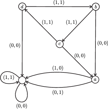
The generators $a,b,c,d$ are defined by one automaton, shown on Figure 3, for different choices of the initial state.

3.3 Non-deterministic automata

Let us generalize the notion of a Mealy automaton by allowing more general Moore diagrams.

Definition 3.5.

A (non-deterministic) synchronous automaton $\mathfrak{A}$ over an alphabet $X$ is an oriented graph whose arrows are labeled by pairs of letters $(x,y)\in X^{2}$ . Such automaton is called $\omega$ -deterministic if for every infinite word $x_{1}x_{2}\ldots\in X^{\omega}$ and for every vertex (i.e., state) $q$ of $\mathfrak{A}$ there exists at most one directed path starting in $q$ which is labeled by $(x_{1},y_{1}),(x_{2},y_{2}),\ldots$ for some $y_{i}\in X$ .

Note that in the above definition for a vertex state $q$ of $\mathfrak{A}$ and a letter $x\in X$ there maybe several or no edges starting at $q$ and labeled by $(x,y)$ for $y\in X$ . It means that the automaton $\mathfrak{A}$ may be non-deterministic on finite words and partial, i.e., that a state $q$ transforms a finite word $v\in X^{*}$ into several different words, and may not accept some of the words on input.

If an automaton $\mathfrak{A}$ is $\omega$ -deterministic, then every its state $q$ defines a map between closed subsets of $X^{\omega}$ , mapping $x_{1}x_{2}\ldots$ to $y_{1}y_{2}\ldots$ , if there exists a directed path starting in $q$ and labeled by $(x_{1},y_{1}),(x_{2},y_{2}),\ldots$ .

Example 3.6.

Let $X=\{0,1\}$ . The states $T_{0}$ and $T_{1}$ of the automaton shown on Figure 4 define the transformations $x_{1}x_{2}\ldots\mapsto 0x_{1}x_{2}\ldots$ and $x_{1}x_{2}\ldots\mapsto 1x_{1}x_{2}\ldots$ , respectively. The states $T_{0}^{\prime}$ and $T_{1}^{\prime}$ define the inverse transformations $0x_{1}x_{2}\ldots\mapsto x_{1}x_{2}\ldots$ and $1x_{1}x_{2}\ldots\mapsto x_{1}x_{2}\ldots$ .

Note that the first automaton (defining the transformations $T_{0}$ and $T_{1}$ ) is deterministic. For example, the state $T_{0}$ acts on the finite words by transformations $x_{1}x_{2}\ldots x_{n}\mapsto 0x_{1}x_{2}\ldots x_{n-1}$ . The second automaton is partial and non-deterministic on finite words. For example, there are two arrows starting at $T_{0}^{\prime}$ labeled by $(0,1)$ and $(0,0)$ , but no arrows labeled by $(1,y)$ .

An asynchronous automaton is defined in the same way, but the labels are pairs of arbitrary words $(u,v)\in(X^{*})^{2}$ .

Definition 3.7.

A homeomorphism $\phi:X^{\omega}\longrightarrow X^{\omega}$ is synchronously (resp. asynchronously) automatic if it is defined by a finite $\omega$ -deterministic synchronous (resp. asynchronous) automaton.

A criterion for a homeomorphism to be synchronously automatic is given in Proposition 4.23.

Asynchronously automatic homeomorphisms of $X^{\omega}$ are studied in [GNS00, GN00]. It is shown there that the set of synchronously automatic homeomorphisms of $X^{\omega}$ is a group, and that it does not depend on $X$ (if $|X|>1$ ). More precisely, it is proved that for any two finite alphabets $X,Y$ (such that $|X|,|Y|>1$ ) there exists a homeomorphism $X^{\omega}\longrightarrow Y^{\omega}$ conjugating the corresponding groups of asynchronously automatic automorphisms. Very little is known about this group, which is called in [GNS00] the group of rational homeomorphisms of the Cantor set.

4 Automatic matrices

4.1 Automatic sequences

Here we review the basic definitions and facts about automatic sequences. More can be found in the monograph [AS03, vH03].

Let $A$ be a finite alphabet, and let $A^{\omega}$ be the space of the right-infinite sequence of elements of $A$ with the direct product topology.

Fix an integer $d\geq 2$ , and consider the transformation $\Xi_{d}:A^{\omega}\longrightarrow(A^{\omega})^{d}$ , which we called the stencil map, defined by the rule

\Xi_{d}(a_{0}a_{1}a_{2}\ldots)=(a_{0}a_{d}a_{2d}\ldots,a_{1}a_{d+1}a_{2d+1}\ldots,\ldots,a_{d-1}a_{2d-1}a_{3d-1}\ldots).

It is easy to see that $\Xi_{d}$ is a homeomorphism. We denote the coordinates of $\Xi_{d}(w)$ by $\Xi_{d}(w)_{i}$ , so that

\Xi_{d}(w)=(\Xi_{d}(w)_{0},\Xi_{d}(w)_{1},\ldots,\Xi_{d}(w)_{d-1}),

and call them $d$ -decimations of the sequence $w$ . Repeated $d$ -decimations of $w$ are all sequences that can be obtained from $w$ by iterative application of the decimation procedure, i.e., all sequences of the form

\Xi_{d}(\Xi_{d}(\ldots\Xi_{d}(w)_{i_{n}}\ldots)_{i_{2}})_{i_{1}}.

Definition 4.1.

A sequence $w\in A^{\omega}$ is $d$ -automatic if the set of all repeated $d$ -decimations of $w$ (called the kernel of $w$ in [AS03, Section 6.6]) is finite.

We say that a subset $Q\subset A^{\omega}$ is $d$ -decimation-closed if for every $w\in Q$ all $d$ -decimations of $w$ belong to $Q$ . The following is obvious.

Lemma 4.2.

A sequence is $d$ -automatic if it belongs to a finite $d$ -decimation-closed subset of $A^{\omega}$ .

Classically, a sequence $w=a_{0}a_{1}\ldots$ is called $d$ -automatic if there exists a Moore automaton $\mathfrak{A}$ with input alphabet $\{0,1,\ldots,d-1\}$ and output alphabet $A$ such that if $n=i_{0}+i_{1}d+\cdots+i_{m}d^{m}$ is a base $d$ expansion of $n$ , then the output of $\mathfrak{A}$ after reading the word $i_{0}i_{1}\ldots i_{m}$ is $a_{n}$ . An equivalent variant of the definition requires that $a_{n}$ is the output of the automaton after reading $i_{m}i_{m-1}\ldots i_{1}i_{0}$ . One also may allow, or not $i_{m}$ to be equal to zero, and the numeration of the letters of the sequence $w$ to start from 1. All these different definitions of automaticity of sequences are equivalent to each other, see [AS03, Section 5.2]. They are also equivalent to Definition 4.1, see [AS03, Theorem 6.6.2].

Example 4.3.

The Thue-Morse sequence is the sequence $t_{0}t_{1}\ldots\in\{0,1\}^{\omega}$ , where $t_{n}$ is the sum modulo 2 of the digits of $n$ in the binary numeration system. The beginning of length $2^{n}$ of this sequence can be obtained from $0$ by applying the substitution

0\mapsto 01,\qquad 1\mapsto 10

$n$ times:

0\mapsto 01\mapsto 0110\mapsto 01101001\mapsto 0110100110010110\mapsto\ldots

It is easy to see that this sequence is generated by the automaton shown on Figure 5. Here we label the vertices (the states) of the automaton by the corresponding values of the output function. The initial state is marked by a double circle. For more on properties of the Thue-Morse sequence, see [AS03, 5.1].

The last example can be naturally generalized to include all automatic sequences. Namely, a $k$ -uniform morphism $\phi:X^{*}\longrightarrow Y^{*}$ is a morphism of monoids such that $|\phi(x)|=k$ for every $x\in X$ . By a theorem of Combham (see [AS03, Theorem 6.3.2]) a sequence is $k$ -automatic if and only if it is an image, under a coding (i.e., a 1-uniform morphism), of a fixed point of a $k$ -uniform endomorphism $\phi:X^{*}\longrightarrow X^{*}$ .

Example 4.4.

Consider the alphabet $X=\{a,b,c\}$ , and the morphism $\phi:X^{*}\longrightarrow X^{*}$ given by

\phi(a)=aca,\quad\phi(b)=d,\quad\phi(c)=b,\quad\phi(d)=c.

This substitution appears in the presentation [Lys85] of the Grigorchuk group.

The fixed point of $\phi$ is obtained as the limit of $\phi^{n}(a)$ , and starts with $acabacadacabaca\ldots$ . The morphism $\phi$ is not uniform, but it is easy to see that the fixed point belongs to $\{ab,ac,ad\}^{\infty}$ , and on the words $B=ab,C=ac,D=ad$ it acts on $\{B,C,D\}^{\infty}$ as a 2-uniform endomorphism:

\phi(B)=acad=CD,\quad\phi(C)=acab=CB,\quad\phi(D)=acac=CC.

It follows from Combham’s theorem that the fixed point of $\phi$ is 2-automatic.

Let us show how to construct an automaton producing a sequence satisfying the conditions of Definition 4.1.

Suppose that $w_{0}\in A^{\omega}$ is automatic, and let $Q$ be a finite $d$ -decimation-closed subset of $A^{\omega}$ that contains $w_{0}$ (for example, we can take $Q$ to be equal to the set of all repeated $d$ -decimations of $w_{0}$ ).

Consider a Moore automaton with the set of states $Q$ , initial state $w_{0}$ , input alphabet $\{0,1,\ldots,d-1\}$ , output alphabet $A$ , transition function

\pi(w,i)=\Xi_{d}(w)_{i},

output function

\tau(x_{0}x_{1}\ldots)=x_{0}.

We call the constructed Moore automaton

\mathfrak{A}=(Q,\{0,1,\ldots,d-1\},A,\pi,\tau,w_{0})

the automaton of $w_{0}$ .

Proposition 4.5.

Let $w_{0}=a_{0}a_{1}\ldots\in A^{\omega}$ be an automatic sequence, and let $\mathfrak{A}$ be its automaton. Let $n$ be a non-negative integer, and let $i_{0},i_{1},\ldots,i_{m}$ be a sequence of elements of the set $\{0,1,\ldots,d-1\}$ such that $n=i_{0}+i_{1}d+i_{2}d^{2}+\cdots+i_{m}d^{m}$ . Then $\tau(w_{0},i_{0}i_{1}\ldots i_{m})=a_{n}$ , i.e., the output of $\mathfrak{A}$ after reading $i_{0}i_{1}\ldots i_{m}$ is $a_{n}$ .

Proof.

It follows from the definition of the automaton $\mathfrak{A}$ that

\pi(w,i_{0}\ldots i_{m})=\Xi_{d}(\ldots\Xi_{d}(\Xi_{d}(x_{0}x_{1}\ldots)_{i_{0}})_{i_{1}}\ldots)_{i_{m}}

(10)

for all $w=x_{0}x_{1}\ldots\in Q$ .

It also follows from the definition of the stencil map that the sequence (10) is equal to

x_{n}x_{n+d^{m+1}}x_{n+2d^{m+1}}x_{n+3d^{m+1}}\ldots,

where $n=i_{0}+i_{1}d+i_{2}d^{2}+\cdots+i_{m}d^{m}$ . It follows that $\tau(w_{0},i_{0}i_{1}\ldots i_{m})=x_{n}$ . ∎

4.2 Automatic infinite matrices

The notion of automaticity of sequences can be generalized to matrices in a straightforward way (see [AS03, Chapter 14], where they are called two-dimensional sequences).

Let $A$ be a finite alphabet, and let $A^{\omega\times\omega}$ be the space of all infinite to right and down two-dimensional matrices of elements of $A$ , i.e., arrays of the form

a=\left(\begin{array}[]{ccc}a_{11}&a_{12}&\ldots\\ a_{21}&a_{22}&\ldots\\ \vdots&\vdots&\ddots\end{array}\right).

(11)

Fix an integer $d\geq 2$ , and consider the map:

\Xi_{d}:A^{\omega\times\omega}\longrightarrow(A^{\omega\times\omega})^{d\times d}

from the set of infinite matrices to the set of $d\times d$ matrices whose entries are elements of $A^{\omega\times\omega}$ . It maps the matrix $a$ to the matrix

\Xi(a)=\left(\begin{array}[]{cccc}\Xi_{d}(a)_{00}&\Xi_{d}(a)_{01}&\ldots&\Xi_{d}(a)_{0,d-1}\\ \Xi_{d}(a)_{10}&\Xi_{d}(a)_{11}&\ldots&\Xi_{d}(a)_{1,d-1}\\ \vdots&\vdots&\ddots&\vdots\\ \Xi_{d}(a)_{d-1,0}&\Xi_{d}(a)_{d-1,1}&\ldots&\Xi_{d}(a)_{d-1,d-1}\end{array}\right),

where

\Xi_{d}(a)_{ij}=\left(\begin{array}[]{cccc}a_{i,j}&a_{i,j+d}&a_{i,j+2d}&\ldots\\ a_{i+d,j}&a_{i+d,j+d}&a_{i+d,j+2d}&\ldots\\ a_{i+2d,j}&a_{i+2d,j+d}&a_{i+2d,j+2d}&\ldots\\ \vdots&\vdots&\vdots&\ddots\end{array}\right).

The entries of $\Xi_{d}(a)$ are called $d$ -decimations of $a$ . We call $\Xi_{d}$ the stencil map, since entries of the matrix $\Xi_{d}(A)$ are obtained from the matrix $A$ by selecting entries using a “stencil” consisting of a square grid of holes, see Figure 6 .

The definition of automaticity for matrices is then the same as for sequences.

Definition 4.6.

A matrix $a\in A^{\omega\times\omega}$ is $d$ -automatic ( $[d,d]$ -automatic in terminology of [AS03]) if the set of matrices that can be obtained from $a$ by repeated $d$ -decimations is finite.

One can also use stencils with a rectangular grid of holes, i.e., selecting the entries of a decimation with one step horizontally, and with a different step vertically. This will lead us to the notion of a $[d_{1},d_{2}]$ -automatic matrix, as in [AS03], but we do not use this notion in our paper.

An interpretation of automaticity of matrices via automata theory is also very similar to the interpretation for sequences. The only difference is that the input alphabet of the automaton is the direct product $\{0,1,\ldots,d-1\}\times\{0,1,\ldots,d-1\}$ . If we want to find an entry $a_{n_{1},n_{2}}$ of an automatic matrix defined by a Moore automaton $\mathfrak{A}$ , then we represent the indices $n_{1}$ and $n_{2}$ in base $d$ :

n_{1}=i_{0}+i_{1}d+\cdots+i_{m}d^{m},\qquad n_{2}=j_{0}+j_{1}d+\cdots+j_{m}d^{m}

for $0\leq i_{s},j_{t}\leq d-1$ , and then feed the sequence $(i_{0},j_{0})(i_{1},j_{1})\ldots(i_{m},j_{m})$ to the automaton $\mathfrak{A}$ . Its final output will be $a_{n_{1},n_{2}}$ .

We say that a matrix $a=(a_{ij})_{i\geq 0,j\geq 0}$ over a field $\Bbbk$ is column-finite if the number of non-zero entries in each column of $a$ is finite. The set $\mathsf{M}_{\infty}(\Bbbk)$ of all column-finite matrices is an algebra isomorphic to the algebra of endomorphisms of the infinite-dimensional vector space $\Bbbk^{\infty}=\bigoplus_{\mathbb{N}}\Bbbk$ . We denote by $\mathsf{M}_{k}(\Bbbk)$ the algebra of $k\times k$ -matrices over $\Bbbk$ .

Lemma 4.7.

The stencil map $\Xi_{d}:\mathsf{M}_{\infty}(\Bbbk)\longrightarrow\mathsf{M}_{d}(\mathsf{M}_{\infty}(\Bbbk))$ is an isomorphism of $\Bbbk$ -algebras.

Proof.

A direct corollary of the multiplication rule for matrices. ∎

Denote by $\mathcal{A}_{d}(\Bbbk)\subset\mathsf{M}_{\infty}(\Bbbk)$ the set of all column-finite $d$ -automatic matrices over $\Bbbk$ .

Proposition 4.8.

Let $\Bbbk$ be a finite field. Then $\mathcal{A}_{d}(\Bbbk)$ is an algebra. The stencil map

\Xi_{d}:\mathcal{A}_{d}(\Bbbk)\longrightarrow\mathsf{M}_{d}(\mathcal{A}_{d}(\Bbbk))

is an isomorphism of $\Bbbk$ -algebras.

Proof.

Let $A$ and $B$ be $d$ -automatic column-finite matrices. Let $\mathfrak{A}$ and $\mathfrak{B}$ be finite decimation-closed sets containing $A$ and $B$ , respectively. Then the set $\{a_{1}A_{1}+b_{1}B_{1}\;:\;A_{1}\in\mathfrak{A},B_{1}\in\mathfrak{B},a_{1},b_{1}\in\Bbbk\}$ is decimation-closed, and it contains any linear combination of $A$ and $B$ . The set is finite, which shows that any linear combination of $A$ and $B$ is automatic.

Let $\mathfrak{C}$ be the linear span of all products $A_{1}B_{1}$ for $A_{1}\in\mathfrak{A}$ , $B_{1}\in\mathfrak{B}$ . Since the stencil map $\Xi_{d}:\mathsf{M}_{\infty}(\Bbbk)\longrightarrow\mathsf{M}_{d}\left(\mathsf{M}_{\infty}(\Bbbk)\right)$ is an isomorphism of $\Bbbk$ -algebras, the set $\mathfrak{C}$ is decimation-closed. It contains $AB$ , hence $AB$ is automatic.

The map $\Xi_{d}:\mathcal{A}_{d}(\Bbbk)\longrightarrow\mathsf{M}_{d}\left(\mathcal{A}_{d}(\Bbbk)\right)$ is obviously a bijection. It is a homomorphism of $\Bbbk$ -algebras, because it is a homomorphism on $\mathsf{M}_{\infty}(\Bbbk)$ . ∎

If we have a finite $d$ -decimation-closed set of matrices $\mathfrak{A}$ , then its elements are uniquely determined by the corresponding matrix recursion $\Xi_{d}:\mathfrak{A}\longrightarrow\mathsf{M}_{d}\left(\mathfrak{A}\right)$ and by the top left entries $a_{00}$ of each matrix $A\in\mathfrak{A}$ . Namely, suppose that we want to find an entry $a_{m,n}$ of a matrix $A\in\mathfrak{A}$ . Let $0\leq i<d$ and $0\leq j<d$ be the remainders of division of $n$ and $m$ by $d$ . Then $a_{m,n}$ is equal to the entry $b_{\frac{m-i}{d},\frac{n-j}{d}}$ of the matrix $B=\Xi_{d}(A)_{i,j}$ . Repeating this procedure several times, we eventually will find a matrix $C=(c_{i,j})_{i,j=0}^{\infty}\in\mathfrak{A}$ such that $a_{m,n}=c_{0,0}$ .

Example 4.9.

A particular case of automatic matrices are triangular matrices of the form

\left(\begin{array}[]{cccc}a_{00}&a_{01}&a_{02}&\ldots\\ 0&a_{11}&a_{12}&\ldots\\ 0&0&a_{22}&\ldots\\ \vdots&\vdots&\vdots&\ddots\end{array}\right),

where the diagonals $a_{0,i},a_{1,i+1},a_{2,i+2},\ldots$ are eventually periodic, and only a finite number of them are non-zero. Note that the set of such uni-triangular matrices is a group.

The following subgroup of this group (of matrices over the field $\mathbb{F}_{2}$ ) was considered in [OS00]. Let $B_{1}=\left(\begin{array}[]{ccc}1&1&1\\ 1&0&0\\ 1&1&1\end{array}\right)$ , $C_{1}=\left(\begin{array}[]{ccc}1&0&0\\ 0&0&0\\ 1&0&0\end{array}\right)$ , $B_{2}=\left(\begin{array}[]{ccc}1&1&0\\ 0&1&0\\ 1&1&0\end{array}\right)$ , $C_{2}=\left(\begin{array}[]{ccc}1&0&0\\ 1&0&0\\ 1&0&0\end{array}\right)$ . It is shown in [OS00] that the infinite matrices

F_{1}=\left(\begin{array}[]{cccccc}I&B_{1}&C_{1}&O&O&\ldots\\ O&I&B_{1}&C_{1}&O&\ldots\\ O&O&I&B_{1}&C_{1}&\ldots\\ \vdots&\vdots&\vdots&\vdots&\vdots&\ddots\end{array}\right),\quad F_{2}=\left(\begin{array}[]{cccccc}I&B_{2}&C_{2}&O&O&\ldots\\ O&I&B_{2}&C_{2}&O&\ldots\\ O&O&I&B_{2}&C_{2}&\ldots\\ \vdots&\vdots&\vdots&\vdots&\vdots&\ddots\end{array}\right)

generate a free group of rank 2. Here $I$ and $O$ are the identity and zero matrices of size $3\times 3$ , respectively.

In Section 5 we will show that any residually finite $p$ -group can be represented in triangular form. Groups generated by finite automata will be represented by automatic uni-triangular matrices. The next subsection is the first step in this direction.

4.3 Representation of automata groups by automatic matrices

Let $\mathsf{B}$ be a basis of $\Bbbk^{X}$ such that $\mathbf{1}\in\mathsf{B}$ . Order the elements of $\mathsf{B}$ into a sequence $y_{0}<y_{1}<\ldots<y_{d-1}$ , where $y_{0}=u$ . Recall that the inductive limit $\mathsf{B}_{\infty}$ of the bases $\mathsf{B}^{\otimes n}$ of $\Bbbk^{X^{n}}$ with respect to the embeddings $f\mapsto f\otimes u$ is a basis of $C(X^{\omega},\Bbbk)$ , whose elements are infinite tensor products $y_{i_{0}}\otimes y_{i_{1}}\otimes\cdots$ , where all but a finite number of factors $y_{i_{k}}$ are equal to $y_{0}=u$ . In other words, $\mathsf{B}_{\infty}$ consists of functions of the form

f(x_{0}x_{1}\ldots)=y_{i_{0}}(x_{0})y_{i_{1}}(x_{1})\cdots,

where all but a finite number of factors on the right-hand side are equal to the constant one function.

We can order such products using the inverse lexicographic order, namely $y_{i_{0}}\otimes y_{i_{1}}\otimes\cdots<y_{j_{0}}\otimes y_{j_{1}}\otimes\cdots$ if and only if $y_{i_{k}}<y_{j_{k}}$ , where $k$ is the largest index such that $y_{i_{k}}\neq y_{j_{k}}$ .

It is easy to see that the ordinal type of $\mathsf{B}_{\infty}$ is $\omega$ . Let $e_{0}<e_{1}<e_{2}<\ldots$ be all elements of $\mathsf{B}_{\infty}$ taken in the defined order. It is checked directly that if $e_{n}=y_{i_{0}}\otimes y_{i_{1}}\otimes\cdots$ , then $n=i_{0}+i_{1}\cdot d+i_{2}\cdot d^{2}+\cdots$ , i.e., $\overline{\ldots i_{2}i_{1}i_{0}}$ is the base- $d$ expansion of $n$ (only a finite number of coefficients $i_{j}$ are different from zero).

Definition 4.10.

An ordered basis $\mathsf{B}$ of $\Bbbk^{X}$ is called marked if its minimal element is $\mathbf{1}$ .

The self-similar basis $\mathsf{B}_{\infty}$ of $C(X^{\omega},\Bbbk)$ associated with $\mathsf{B}$ is the inverse lexicographically ordered set of functions of the form $e_{1}\otimes e_{2}\otimes\ldots$ , where $e_{i}\in\mathsf{B}$ and all but a finite set of elements $e_{i}$ are equal to $\mathbf{1}$ , as it is described above.

Let $\mathsf{B}=\{b_{0},b_{1},\ldots,b_{d-1}\}$ be an arbitrary (non necessarily marked) basis of the space $\Bbbk^{X}$ . We define the associated matrix recursion for linear operators on $C(X^{\omega},\Bbbk)$ in the usual way: given an operator $a$ , define its image $\Xi_{\mathsf{B}}(a)=(A_{i,j})_{i,j=0}^{d-1}$ in $\mathsf{M}_{d}(C(X^{\omega},\Bbbk)$ by the rule

a(b_{j}\otimes f)=\sum_{i=0}^{d-1}b_{i}\otimes A_{i,j}(f),\qquad f\in C(X^{\omega},\Bbbk),0\leq j\leq d-1.

If $\mathsf{B}$ is the basis $\{\delta_{x}\}_{x\in X}$ , then the matrix recursion $\Xi_{\mathsf{B}}$ restricted to a self-similar group $G\leq\mathop{\mathrm{Aut}}(X^{*})$ coincides with the matrix recursion (5) coming directly from the wreath recursion.

Lemma 4.11.

Let $\mathsf{B}$ be a marked basis of $\Bbbk^{X}$ . Then the matrix recursion $\Xi_{\mathsf{B}}$ coincides with the stencil map for the matrices of linear operators in the associated basis $\mathsf{B}_{\infty}$ .

Proof.

Let $A_{ij}$ , $0\leq i,j\leq d-1$ , be the entries of $\Xi_{\mathsf{B}}(a)$ . Let $n=i_{0}+i_{1}\cdot d+i_{2}\cdot d^{2}+\cdots$ be a non-negative integer written in base $d$ . Then

a(b_{j+dn})=a(b_{j}\otimes b_{n})=\sum_{i=0}^{d-1}b_{i}\otimes A_{i,j}(b_{n}).

(12)

Let $a_{m,n}$ , $0\leq m,n<\infty$ , be the entries of the matrix of $a$ in the basis $\mathsf{B}_{\infty}$ . Then

a(b_{j+dn})=\sum_{k=0}^{\infty}a_{k,j+dn}b_{k}=\sum_{i=0}^{d-1}\sum_{r=0}^{\infty}a_{i+dr,j+dn}b_{i}\otimes b_{r}=\sum_{i=0}^{d-1}b_{i}\otimes\left(\sum_{r=0}^{\infty}a_{i+dr,j+dn}b_{r}\right),

which together with (12) implies that $c_{r,n}=a_{i+dr,j+dn}$ are the entries of $A_{i,j}$ in the basis $\mathsf{B}_{\infty}$ , i.e., that $A_{i,j}=\Xi_{d}(a)_{i,j}$ . ∎

Definition 4.12.

Let $\Bbbk$ be a finite field. We say that a linear operator $a$ on $C(X^{\omega},\Bbbk)$ is automatic if there exists a finite set $\mathfrak{A}$ of operators such that $a\in\mathfrak{A}$ , and for every $a^{\prime}\in\mathfrak{A}$ all entries of the matrix $\Xi_{\mathsf{B}}(a^{\prime})$ belong to $\mathfrak{A}$ .

Proposition 4.13.

Let $\mathsf{B}_{1},\mathsf{B}_{2}$ be two bases of $\Bbbk^{X}$ . An linear operator on $C(X^{\omega},\Bbbk)$ is automatic with respect to $\mathsf{B}_{1}$ if and only if it is automatic with respect to $\mathsf{B}_{2}$ .

Proof.

Let $a_{1}$ be an operator which is automatic with respect to $\mathsf{B}_{1}$ . Let $\mathfrak{A}$ be the corresponding finite set of operators, closed with respect to taking entries of the matrix recursion. Let $\mathfrak{A}^{\prime}$ be the set of all linear combinations of elements of $\mathfrak{A}$ , which is finite, since we assume that $\Bbbk$ is finite. If $T$ is the transition matrix from $\mathfrak{B}_{1}$ to $\mathfrak{B}_{2}$ , then

\Xi_{\mathfrak{B}_{2}}(a)=T^{-1}\Xi_{\mathfrak{B}_{1}}(a)T

for every linear operator $a$ . It follows that $\mathfrak{A}^{\prime}$ is closed with respect to taking entries of $\Xi_{\mathfrak{B}_{2}}$ . The set $\mathfrak{A}^{\prime}$ is finite, $a_{1}\in\mathfrak{A}^{\prime}$ , hence $a_{1}$ is also automatic with respect to $\mathsf{B}_{2}$ . ∎

As a direct corollary of Proposition 4.13 we get the following relation between finite-state automorphisms of the rooted tree $X^{*}$ and automatic matrices.

Theorem 4.14.

Suppose that $\Bbbk$ is finite. Let $\mathsf{B}$ be a marked basis of $\Bbbk^{X}$ . Then the matrix of $\pi_{\infty}(g)$ in the associated basis $\mathsf{B}_{\infty}$ , where $g\in\mathop{\mathrm{Aut}}(X^{*})$ , is $d$ -automatic if and only if $g$ is finite-state.

We get, therefore, a subgroup of the group of units of $\mathcal{A}_{d}(\Bbbk)$ isomorphic to the group $\mathop{\mathrm{FAut}}(X^{*})$ of finite-state automorphisms of the tree $X^{*}$ .

Matrix recursions (i.e., homomorphisms from an algebra $A$ to the algebra of matrices over $A$ ) associated with groups acting on rooted trees, and in more general cases were studied in many papers, for instance in [Sid97, BG00b, Bar06, Sid09, Bac08, Nek04, Nek09]. Note that the algebra generated by the natural representation on $C(X^{\omega},\Bbbk)$ of a group $G$ acting on the rooted tree $X^{*}$ is different from the group ring. This algebra (and its analogs) were studied in [Sid97, Bar06, Nek04].

4.4 Creation and annihilation operators

For $h\in\Bbbk^{X}$ , denote by $T_{h}$ the operator on $C(X^{\omega},\Bbbk)$ acting by the rule

T_{h}(f)=h\otimes f.

It is easy to see that $T_{h}$ is linear, and that we have $T_{a_{1}h_{1}+a_{2}h_{2}}=a_{1}T_{h_{1}}+a_{2}T_{h_{2}}$ for all $h_{1},h_{2}\in\Bbbk^{X}$ and $a_{1},a_{2}\in\Bbbk$ .

Consider the dual vector space $(\Bbbk^{X})^{\prime}$ to the space $\Bbbk^{X}$ of functions. We will denote the value of a functional $v$ on a function $f\in\Bbbk^{X}$ by $\langle v|f\rangle$ . Then for every $v\in(\Bbbk^{X})^{\prime}$ we have an operator $T_{v}$ on $C(X^{\omega},\Bbbk)$ defined by

T_{v}(f)(x_{1},x_{2},\ldots)=\langle v|f(x,x_{1},x_{2},\ldots)\rangle,

where $f(x,x_{1},x_{2},\ldots)$ on the right-hand side of the equation is seen for every choice of the variables $x_{1},x_{2},\ldots$ as a function of one variable $x$ , i.e., an element of $\Bbbk^{X}$ .

Let $\mathsf{B}=\{e_{i}\}_{i=0}^{d-1}$ be a basis of $\Bbbk^{X}$ . Let $\mathsf{B}^{\prime}=\{e_{i}^{\prime}\}_{i=0}^{d-1}$ be the basis of the dual space defined by $\langle e_{i}^{\prime}|e_{j}\rangle=\delta_{i,j}$ . (Here and in the sequel, $\delta_{i,j}$ is the Kronecker’s symbol equal to 1 when $i=j$ , and to 0 otherwise.) We will denote $T_{e_{i}^{\prime}}=T_{e_{i}}^{\prime}$ .

Then $T_{e_{i}}$ is an isomorphism between the space $C(X^{\omega},\Bbbk)$ and its subspace $e_{i}\otimes C(X^{\omega},\Bbbk)$ . It is easy to see that $T_{e_{i}}^{\prime}$ restricted onto $e_{i}\otimes C(X^{\omega},\Bbbk)$ is the inverse of this isomorphism, and that $T_{e_{i}}^{\prime}$ restricted onto $e_{j}\otimes C(X^{\omega},\Bbbk)$ is equal to zero for $j\neq i$ .

The operators $T_{e_{i}}$ and $T_{e_{j}}^{\prime}$ satisfy the relations:

T_{e_{i}}^{\prime}T_{e_{j}}=\delta_{e_{i},e_{j}},\qquad\sum_{e_{i}\in\mathsf{B}}T_{e_{i}}T_{e_{i}}^{\prime}=1.

(13)

The products $T_{e_{i}}T_{e_{i}}^{\prime}$ are projections onto the summands $e_{i}\otimes C(X^{\omega},\Bbbk)$ of the direct sum decomposition

C(X^{\omega},\Bbbk)=\bigoplus_{e_{i}\in\mathsf{B}}e_{i}\otimes C(X^{\omega},\Bbbk).

Let $\mathsf{B}$ be a marked basis of $\Bbbk^{X}$ , and let $\mathbf{1}=e_{0}<e_{1}<\ldots<e_{d-1}$ be its elements. Let $\mathsf{B}_{\infty}$ be the associated ordered basis of $C(X^{\omega},\Bbbk)$ .

If $A$ is (not necessarily square) finite matrix, then we denote by $A^{\oplus\infty}$ the infinite matrix

\left(\begin{array}[]{cccc}A&O&O&\ldots\\ O&A&O&\ldots\\ O&O&A&\ldots\\ \vdots&\vdots&\vdots&\ddots\end{array}\right),

where $O$ is the zero matrix of the same size as $A$ .

The following is a direct corollary of the definitions.

Proposition 4.15.

The matrices of $T_{e_{0}}$ , $T_{e_{1}}$ , …, $T_{e_{d-1}}$ in the basis $\mathsf{B}$ are equal to

E_{0}=\left(\begin{array}[]{c}1\\ 0\\ \vdots\\ 0\end{array}\right)^{\oplus\infty},E_{1}=\left(\begin{array}[]{c}0\\ 1\\ \vdots\\ 0\end{array}\right)^{\oplus\infty},\ldots,E_{d-1}=\left(\begin{array}[]{cccc}0\\ 0\\ \vdots\\ 1\end{array}\right)^{\oplus\infty},

respectively. The matrix of $T_{e_{i}}^{\prime}$ is the transpose $E_{i}^{\top}$ of the matrix $E_{i}$ .

The matrices $E_{i}$ and $E_{i}^{\prime}$ have a natural relation to decimation of matrices. The proof of the next proposition is a straightforward computation of matrix products.

Proposition 4.16.

Let $A=(a_{i,j})_{i,j=0}^{\infty}$ be an infinite matrix, and let

\Xi_{d}(A)=\left(\begin{array}[]{cccc}A_{0,0}&A_{0,1}&\ldots&A_{0,d-1}\\ A_{1,0}&A_{1,1}&\ldots&A_{1,d-1}\\ \vdots&\vdots&\ddots&\vdots\\ A_{d-1,0}&A_{d-1,1}&\ldots&A_{d-1,d-1}\end{array}\right)

be the matrix of its $d$ -decimations. Then

A_{i,j}=E_{i}^{\prime}AE_{j}

and

A=\sum_{i,j=0}^{d-1}E_{i}A_{i,j}E_{j}^{\prime}.

Corollary 4.17.

Let $A$ be an operator on $C(X^{\omega},\Bbbk)$ , and let $\mathsf{B}=\{e_{i}\}$ be a basis of $\Bbbk^{X}$ . Then the entries of the associated matrix recursion for $A$ are equal to $T_{e_{i}}^{\prime}AT_{e_{j}}$ .

The next proposition is a direct corollary of Proposition 4.15.

Proposition 4.18.

If $h=a_{0}e_{0}+a_{1}e_{1}+\cdots+a_{d-1}e_{d-1}$ , then the matrix of $T_{h}$ is equal to $\left(\begin{array}[]{c}a_{0}\\ a_{1}\\ \vdots\\ a_{d-1}\end{array}\right)^{\oplus\infty}.$

Corollary 4.19.

Let $\mathsf{B}$ be a marked basis of $\Bbbk^{X}$ . Order the letters of the alphabet $X$ in a sequence $x_{0},x_{1},\ldots,x_{d-1}$ . Let $T_{i}=T_{\delta_{x_{i}}}$ and $T_{i}^{\prime}=T_{\delta_{x_{i}}}^{\prime}$ be the corresponding operators, defined using the basis $\{\delta_{x_{i}}\}$ .

Let $S=(a_{ij})_{i,j=0}^{d-1}$ be the transition matrix from the basis $\delta_{x_{0}}<\delta_{x_{1}}<\cdots<\delta_{x_{d-1}}$ to $\mathsf{B}$ . Let $S^{-1}=(b_{ij})_{i,j=0}^{d-1}$ be the inverse matrix.

Then the matrix of $T_{i}$ is

\left(\begin{array}[]{c}b_{0,i}\\ b_{1,i}\\ \ldots\\ b_{d-1,i}\end{array}\right)^{\oplus\infty},

and the matrix of $T_{i}^{\prime}$ is

\left(\begin{array}[]{cccc}a_{i,0}&a_{i,1}&\ldots&a_{i,d-1}\end{array}\right)^{\oplus\infty}.

Let us consider now the case of the basis $\mathsf{D}=\{\delta_{x}\}_{x\in X}$ . For simplicity, let us denote $T_{x}=T_{\delta_{x}}$ and $T_{x}^{\prime}=T_{\delta_{x}}^{\prime}$ . Then the operators $T_{x}$ and $T_{x}^{\prime}$ act on $C(X^{\omega},\Bbbk)$ by the rule

T_{x}(f)(x_{1},x_{2},\ldots)=\left\{\begin{array}[]{ll}f(x_{2},x_{3},\ldots)&\text{if $x=x_{1}$,}\\ 0&\text{otherwise.}\end{array}\right.

(14)

and

T_{x}^{\prime}(f)(x_{1},x_{2},\ldots)=f(x,x_{1},x_{2},\ldots).

(15)

In other words, the operator $T_{x}$ is induced by the natural homeomorphism $X^{\omega}\longrightarrow xX^{\omega}:w\mapsto xw$ , and $T_{x}^{\prime}$ is induced by its inverse map $xX^{\omega}\longrightarrow X^{\omega}:xw\mapsto w$ .

Proposition 4.20.

Let $\mathsf{B}_{\infty}$ be a self-similar basis of $C(X^{\omega},\Bbbk)$ associated with a marked basis $\mathsf{B}$ (see Definition 4.10). Then the matrices of the operators $T_{x}$ and $T_{x}^{\prime}$ , for $x\in X$ , in the ordered basis $\mathsf{B}_{\infty}$ are $|X|$ -automatic.

Note that we do not require in this proposition the field $\Bbbk$ to be finite.

Proof.

Let $\delta_{x}=\sum_{i=0}^{d-1}\alpha_{x,i}e_{i}$ for $x\in X$ , $\mathsf{B}=\{e_{i}\}_{i=0}^{d-1}$ and $\alpha_{x,i}\in\Bbbk$ . It follows from Proposition 4.16 that the entries of the matrix $\Xi_{2}(T_{x})$ with respect to the basis $\mathsf{B}$ are equal to $\sum_{k=0}^{d-1}\alpha_{x,k}T_{e_{i}}^{\prime}T_{e_{k}}T_{e_{j}}$ . Every product of the form $T_{e_{i}}^{\prime}T_{e_{k}}T_{e_{j}}$ is equal, by relations (13), either to zero, or to $T_{e_{j}}$ . It follows that decimations of $T_{x}$ are either zeros or of the form $\alpha_{x,i}T_{e_{j}}$ . It follows that the set of repeated decimations of the matrix of $T_{x}$ is contained in $\{\alpha_{x,0},\alpha_{x,1},\cdots,\alpha_{x,d-1}\}\cdot\{T_{e_{0}},T_{e_{1}},\ldots,T_{e_{d-1}}\}\cup\{0\}$ . ∎

Example 4.21.

Let us consider the case $X=\{0,1\}$ and $\mathsf{B}=\{y_{0},y_{1}\}$ , where $y_{0}=\delta_{0}+\delta_{1}$ and $y_{1}=\delta_{1}$ . Then the transition matrix from $\{\delta_{0},\delta_{1}\}$ to $\{y_{0},y_{1}\}$ is $\left(\begin{array}[]{cc}1&0\\ 1&1\end{array}\right)$ , whose inverse is $\left(\begin{array}[]{cc}1&0\\ -1&1\end{array}\right)$ .

It follows then from Corollary 4.19 that the matrices of $T_{0}$ , $T_{1}$ , $T_{0}^{\prime}$ , and $T_{1}^{\prime}$ in the basis $\mathsf{B}_{\infty}$ are

T_{0}=\left(\begin{array}[]{r}1\\ -1\end{array}\right)^{\oplus\infty},\quad T_{1}=\left(\begin{array}[]{c}0\\ 1\end{array}\right)^{\oplus\infty},

and

T_{0}^{\prime}=\left(\begin{array}[]{cc}1&0\end{array}\right)^{\oplus\infty},\quad T_{1}^{\prime}=\left(\begin{array}[]{cc}1&1\end{array}\right)^{\oplus\infty}.

Example 4.22.

In the case $\Bbbk=\mathbb{C}$ , it is natural to consider the operators

S_{x}=\frac{1}{\sqrt{|X|}}T_{x}.

Then $S_{x}$ are isometries of the Hilbert space $L^{2}(X^{\omega})$ , and their conjugates $S_{x}^{*}$ are equal to $\sqrt{|X|}T_{x}^{\prime}$ .

The $C^{*}$ -algebra of operators on $L^{2}(X^{\omega})$ generated by the operators $S_{x}$ is called the Cuntz algebra [Cun77], and is usually denoted $\mathcal{O}_{|X|}$ . Any isometries satisfying the relations

S_{x}^{*}S_{x}=1,\qquad\sum_{x\in X}S_{x}S_{x}^{*}=1

generate a $C^{*}$ -algebra isomorphic to $\mathcal{O}_{|X|}$ . In particular, the $C^{*}$ -algebra generated by the matrices $E_{i}$ is the Cuntz algebra. Representation of the Cuntz algebra by matrices $E_{i}$ is an example of a permutational representation of $\mathcal{O}_{d}$ . More on such and similar representations, see [BJ99].

Recall that, for $X=\{0,1\}$ , the Walsh basis of $L^{2}(X^{\omega})$ is the basis $\mathsf{W}_{\infty}$ constructed starting from the basis $\mathsf{W}=\{y_{0},y_{1}\}$ , where $y_{0}=\delta_{0}+\delta_{1}$ and $y_{1}=\delta_{0}-\delta_{1}$ . Then direct computation with of the transition matrices show that the matrices of $S_{0}$ and $S_{1}$ are

S_{0}=\left(\begin{array}[]{c}\frac{1}{\sqrt{2}}\\ \frac{1}{\sqrt{2}}\end{array}\right)^{\oplus\infty},\qquad S_{1}=\left(\begin{array}[]{r}\frac{1}{\sqrt{2}}\\ -\frac{1}{\sqrt{2}}\end{array}\right)^{\oplus\infty}.

4.5 Cuntz algebras and Higman-Thompson groups

If $\psi:X^{\omega}\longrightarrow X^{\omega}$ is a homeomorphism, then it induces a linear operator $L_{\psi}$ on $C(X^{\omega},\Bbbk)$ given by

L_{\psi}(f)(w)=f(\psi^{-1}(w))

for $f\in C(X^{\omega},\Bbbk)$ and $w\in X^{\omega}$ .

Fixing any ordered basis of $C(X^{\omega},\Bbbk)$ , we get thus a natural faithful representation of the homeomorphism group of $X^{\omega}$ in the group of units of the algebra $\mathsf{M}_{\infty}(\Bbbk)$ of column-finite matrices over $\Bbbk$ .

Proposition 4.23.

Let $\psi$ be a homeomorphism of $X^{\omega}$ . Let $u,v\in X^{n}$ , and denote by $\psi_{u,v}$ the partially defined map given by the formula

\psi_{u,v}(w)=\left\{\begin{array}[]{ll}w^{\prime}&\text{if $\psi(vw)=uw^{\prime}$,}\\ \text{not defined}&\text{otherwise.}\end{array}\right.

The following conditions are equivalent.

1.

The homeomorphism $\psi$ is synchronously automatic.
2.

The set of partial maps $\{\psi_{u,v}\;:\;u,v\in X^{*},|u|=|v|\}$ is finite.
3.

For every finite field $\Bbbk$ , the operator $L_{\psi}:C(X^{\omega},\Bbbk)\longrightarrow C(X^{\omega},\Bbbk)$ is automatic.
4.

For some finite field $\Bbbk$ , the operator $L_{\psi}:C(X^{\omega},\Bbbk)\longrightarrow C(X^{\omega},\Bbbk)$ is automatic.

Synchronously automatic homeomorphisms are defined in Definition 3.7.

Proof.

Equivalence of conditions (2), (3), and (5) follow directly from Proposition 4.16.

Suppose that $\psi$ is synchronously automatic. Let $\mathfrak{A}$ be an initial automaton defining $\psi$ . For every pair $u=a_{1}a_{2}\ldots a_{n},v=b_{1}b_{2}\ldots b_{n}\in X^{*}$ of words of equal length, let $Q_{u,v}$ be the set of states $q$ of $\mathfrak{A}$ such that there exists a directed path starting in the initial state $q_{0}$ of $\mathfrak{A}$ and labeled by $(a_{1},b_{1}),(a_{2},b_{2}),\ldots,(a_{n},b_{n})$ . Then the set $Q_{u,v}$ defines the map $\psi_{u,v}$ in the following sense. We have $\psi_{u,v}(x_{1}x_{2}\ldots)=y_{1}y_{2}\ldots$ if and only if there exists a path starting in an element of $Q_{u,v}$ and labeled by $(x_{1},y_{1}),(x_{2},y_{2}),\ldots$ . It follows that the number of possible maps of the form $\psi_{u,v}$ is not larger than the number of subsets of the set of states of $\mathfrak{A}$ . This shows that every synchronously automatic homeomorphism satisfies condition (2).

Suppose now that a homeomorphism $\psi$ satisfies condition (2), and let us show that it is synchronously automatic. Construct an automaton $\mathfrak{A}$ with the set of states $Q$ equal to the set of non-empty maps of the form $\psi_{u,v}$ . For every $(x,y)\in X^{2}$ and $\psi_{u,v}\in Q$ we have an arrow from $\psi_{u,v}$ to $\psi_{ux,vy}$ , labeled by $(x,y)$ , provided the map $\psi_{ux,vy}$ is not empty. The initial state of the automaton is the map $\psi=\psi_{\emptyset,\emptyset}$ . Let us show that this automaton defines the homeomorphism $\psi$ . It is clear that if $\psi(x_{1}x_{2}\ldots)=y_{1}y_{2}\ldots$ , then there exists a path starting at the initial state of $\mathfrak{A}$ and labeled by $(x_{1},y_{1}),(x_{2},y_{2}),\ldots$ . On the other hand, if such a path exists for a pair of infinite words $x_{1}x_{2}\ldots,y_{1}y_{2}\ldots$ , then the maps $\psi_{x_{1}x_{2}\ldots x_{n},y_{1}y_{2}\ldots y_{n}}$ are non-empty for every $n$ . In other words, for every $n$ the set $W_{n}$ of infinite sequences $w\in x_{1}x_{2}\ldots x_{n}X^{\omega}$ such that $\psi(w)\in y_{1}y_{2}\ldots y_{n}X^{\omega}$ is non-empty. It is clear that the sets $W_{n}$ are closed and $W_{n+1}\subset W_{n}$ for every $n$ . By compactness of $X^{\omega}$ it implies that $\bigcap_{n\geq 1}W_{n}$ is non-empty. It follows that $\psi(x_{1}x_{2}\ldots)=y_{1}y_{2}\ldots$ . ∎

The next corollary follows directly from condition (2) of Proposition 4.23.

Corollary 4.24.

The set of all automatic homeomorphisms of $X^{\omega}$ is a group.

We have already seen in Theorem 4.14 that a homeomorphisms $g$ of $X^{\omega}$ defined by an automorphisms of $X^{*}$ is automatic if and only if it is finite state. Note that in this case $g_{u,v}$ is either empty (if $g(v)\neq u$ ) or is equal to $g|_{v}$ .

Another example of a group of finitely automatic homeomorphisms of $X^{\omega}$ is the Higman-Thompson group $\mathcal{V}_{|X|}$ . It is the set of all homeomorphisms that can be defined in the following way. We say that a subset $A\subset X^{*}$ is a cross-section if the sets $uX^{\omega}$ for $u\in A$ are disjoint and their union is $X^{\omega}$ . Let $A=\{v_{1},v_{2},\ldots,v_{n}\}$ and $B=\{u_{1},u_{2},\ldots,u_{n}\}$ be cross-sections of equal cardinality together with a bijection $v_{i}\mapsto u_{i}$ . Define a homeomorphism $\psi:X^{\omega}\longrightarrow X^{\omega}$ by the rule

\psi(v_{i}w)=u_{i}w.

(16)

The set of all homeomorphisms that can be defined in this way is the Higman-Thompson group $\mathcal{V}_{|X|}$ , see [Tho80, CFP96].

Let $\psi$ be the homeomorphism defined by (16). It follows directly from (14) and (15) that the operator $L_{\psi}$ induced by $\psi$ is equal to

L_{\psi}=\sum_{i=1}^{n}T_{u_{i}}T_{v_{i}}^{\prime},

where we use notation

T_{x_{1}x_{2}\ldots x_{m}}=T_{x_{1}}T_{x_{2}}\cdots T_{x_{n}},\qquad T_{x_{1}x_{2}\ldots x_{m}}^{\prime}=T_{x_{m}}^{\prime}T_{x_{m-1}}^{\prime}\cdots T_{x_{1}}^{\prime}.

The next proposition follows then from Proposition 4.20.

Proposition 4.25.

The Higman-Thompson group $\mathcal{V}_{|X|}$ is a subgroup of the group of synchronously automatic homeomorphisms of $X^{\omega}$ .

The group generated by $\mathcal{V}_{2}$ and the Grigorchuk group was studied by K. Roever in [Röv99]. He proved that it is a finitely presented simple group isomorphic to the abstract commensurizer of the Grigorchuk group. Generalizations of this group (for arbitrary self-similar group) was studied in [Nek04].

5 Representations by uni-triangular matrices

5.1 Sylow $p$ -subgroup of $\mathop{\mathrm{Aut}}(X^{*})$

Let $|X|=p$ be prime. We assume that $X=\{0,1,\ldots,p-1\}$ is equal to the field $\mathbb{F}_{p}$ of $p$ elements. From now on, we will write vertices of the tree $X^{*}$ as tuples $(x_{1},x_{2},\ldots,x_{n})$ in order not to confuse them with products of elements of $\mathbb{F}_{p}$ .

Denote by $\mathcal{K}_{p}$ the subgroup of $\mathop{\mathrm{Aut}}(X^{*})$ consisting of automorphisms $g$ whose labels $\alpha_{g,v}$ of the vertices of the portrait consist only of powers of the cyclic permutation $\sigma=(0,1,\ldots,p-1)$ . It follows from (2) and (3) that $\mathcal{K}_{p}$ is a group. The study of the group $\mathcal{K}_{p}$ (and its finite analogs were initiated by L. Kaloujnine [Kal48, Kal47, Kal51]).

Suppose that an element $g\in\mathcal{K}_{p}$ is represented by a tableau

[a_{0},a_{1}(x_{1}),a_{2}(x_{1},x_{2}),\ldots],

as in Subsection 2.1. Then $a_{n}(x_{1},x_{2},\ldots,x_{n})$ are maps from $X^{n}$ to the group generated by the cyclic permutation $\sigma$ . The elements of this group act on $X=\mathbb{F}_{p}$ by maps $\sigma^{a}:x\mapsto x+a$ . It follows that we can identify functions $a_{n}$ with maps $X^{n}\longrightarrow\mathbb{F}_{p}$ , so that an element $g\in\mathcal{K}_{p}$ represented by a tableau

[a_{0},a_{1}(x_{1}),a_{2}(x_{1},x_{2}),\ldots]

acts on sequences $v=(x_{0},x_{1},\ldots)\in X^{\omega}$ by the rule

g(v)=(x_{0}+a_{0},x_{1}+a_{1}(x_{0}),x_{2}+a_{2}(x_{1},x_{2}),x_{3}+a_{3}(x_{1},x_{2},x_{3}),\ldots).

It follows that if $g_{1},g_{2}\in\mathcal{K}_{p}$ are represented by the tableaux $[a_{n}]_{n=0}^{\infty}$ and $[b_{n}]_{n=0}^{\infty}$ , then their product $g_{1}g_{2}$ is represented by the tableau

[b_{0}+a_{0},\quad b_{1}(x_{0})+a_{1}(x_{0}+b_{0}),\\ b_{2}(x_{0},x_{1})+a_{2}(x_{0}+b_{0},x_{1}+b_{1}(x_{0})),\\ b_{3}(x_{0},x_{1},x_{2})+a_{3}(x_{0}+b_{0},x_{1}+b_{1}(x_{0}),x_{2}+b_{2}(x_{0},x_{1})),\quad\ldots].

(17)

Denote by $\mathcal{K}_{p,n}$ the quotient of $\mathcal{K}_{p}$ by the pointwise stabilizer of the $n$ th level of the tree $X^{*}$ . We can consider $\mathcal{K}_{p,n}$ as a subgroup of the automorphism group of the finite subtree $X^{[n]}=\bigcup_{k=0}^{n}X^{k}\subset X^{*}$ .

Proposition 5.1.

The group $\mathcal{K}_{p,n}$ is a Sylow subgroup of the symmetric group $\mathop{\mathrm{Symm}}(X^{n})$ and of the automorphism group of the tree $X^{[n]}$ .

Proof.

The order of $\mathop{\mathrm{Symm}}(X^{n})$ is $p^{n}!$ , and the maximal power of $p$ dividing it is

\frac{p^{n}}{p}+\frac{p^{n}}{p^{2}}+\cdots+\frac{p^{n}}{p^{n}}=\frac{p^{n}-1}{p-1}.

It follows that the order of the Sylow $p$ -subgroup of $\mathop{\mathrm{Symm}}(X^{n})$ is $p^{\frac{p^{n}-1}{p-1}}$ . The order of $\mathcal{K}_{p,n}$ is equal to the number of possible tableaux

[a_{0},a_{1}(x_{1}),a_{2}(x_{1},x_{2}),\ldots a_{n-1}(x_{1},\ldots,x_{n-1})],

where $a_{i}$ is an arbitrary map from $X^{i}$ to the cyclic group $\langle\sigma\rangle$ of order $p$ . The number of possibly maps $a_{i}$ is hence $p^{p^{i}}$ . Consequently, the number of possible tableaux is $p^{1+p+p^{2}+\cdots+p^{n-1}}=p^{\frac{p^{n}-1}{p-1}}$ . Since the group of all automorphisms of the tree $X^{[n]}$ is contained in $\mathop{\mathrm{Symm}}(X^{n})$ and contains $\mathcal{K}_{p,n}$ , the subgroup $\mathcal{K}_{p,n}$ is its Sylow $p$ -subgroup too. ∎

Proposition 5.2.

Let $g\in\mathcal{K}_{p}$ be represented by a tableau $[a_{0},a_{1}(x_{1}),a_{2}(x_{1},x_{2}),\ldots]$ . Consider the map $\alpha:\mathcal{K}_{p}\longrightarrow\mathbb{F}_{p}^{\omega}$ , where $\mathbb{F}_{p}^{\omega}$ is the infinite Cartesian product of additive groups of $\mathbb{F}_{p}$ , given by

\alpha(g)=\left(a_{0},\sum_{x_{1}\in\mathbb{F}_{p}}a_{1}(x_{1}),\sum_{(x_{1},x_{2})\in\mathbb{F}_{p}^{2}}a_{2}(x_{1},x_{2}),\ldots\right).

(18)

In other words, we just sum up modulo $p$ all the decorations of the portrait of $g$ on each level. Then $\alpha$ is the abelianization epimorphism $\mathcal{K}_{p}\longrightarrow\mathcal{K}_{p}/[\mathcal{K}_{p},\mathcal{K}_{p}]\cong\mathbb{F}_{p}^{\omega}$ .

Proof.

It is easy to check that $\alpha$ is a homomorphism. It remains to show that its kernel is the derived subgroup of $\mathcal{K}_{p}$ . This is a folklore fact, and we show here how it follows from a more general result of Kaloujnine.

Let $g\in\mathcal{K}_{p}$ be represented by a tableau

[a_{0},a_{1}(x_{1}),a_{2}(x_{1},x_{2}),\ldots].

Each function $a_{n}(x_{1},x_{2},\ldots,x_{n})$ can be written as a polynomial

\sum_{0\leq k_{i}\leq p-1}c_{k_{1},k_{2},\ldots,k_{n}}x_{1}^{k_{1}}x_{2}^{k_{2}}\cdots x_{n}^{k_{n}}

for some coefficients $c_{k_{1},k_{2},\ldots,k_{n}}\in\mathbb{F}_{p}$ .

It is proved in [Kal48, Theorem 6] (see also Equation (5,4) in [Kal51]) that the derived subgroup $[\mathcal{K}_{p},\mathcal{K}_{p}]$ of $\mathcal{K}_{p}$ is the set of elements defined by tableaux in which $a_{0}$ and the coefficient $c_{p-1,p-1,\ldots,p-1}$ at the eldest term $x_{1}^{p-1}x_{2}^{p-1}\ldots x_{n}^{p-1}$ are equal to zero for every $n$ .

Note that $\sum_{x\in\mathbb{F}_{p}}x^{k}$ is equal to zero for $k=0,1,\ldots,p-2$ and is equal to $-1$ for $k=p-1$ . Therefore,

\sum_{(x_{1},x_{2},\ldots,x_{n})\in\mathbb{F}_{p}^{n}}x_{1}^{k_{1}}x_{2}^{k_{2}}\cdots x_{n}^{k_{n}}=\prod_{i=1}^{n}\sum_{x\in\mathbb{F}_{p}}x^{k_{i}}

is equal to zero for all $n$ -tuples $(k_{1},k_{2},\ldots,k_{n})\in\{0,1,\ldots,p-1\}^{n}$ except for $(p-1,p-1,\ldots,p-1)$ , when it is equal to $(-1)^{n}$ . It follows that the coefficient at the eldest term of $a_{n}(x_{1},x_{2},\ldots,x_{n})$ is equal to zero if and only if $\sum_{(x_{1},x_{2},\ldots,x_{n})\in\mathbb{F}_{p}^{n}}a_{n}(x_{1},x_{2},\ldots,x_{n})=0$ . ∎

5.2 Polynomial bases of $C(X^{\omega},\mathbb{F}_{p})$

Proposition 5.3.

Suppose that an ordered basis $\mathsf{B}$ of $\Bbbk^{X}$ is such that the matrices of $\pi_{1}(g)$ for $g\in G\leq\mathop{\mathrm{Aut}}(X^{*})$ are all upper uni-triangular, and the minimal element of $\mathsf{B}$ is the constant one function. Then the matrices of $\pi_{n}(g)$ in the basis $\mathsf{B}^{\otimes n}$ and of $\pi_{\infty}(g)$ in the associated basis $\mathsf{B}_{\infty}$ are upper uni-triangular for all $g\in G$ .

See Subsection 2.4 for definition of the representations $\pi_{n}$ . We say that a matrix is upper uni-triangular if all its elements below the main diagonal are equal to zero, and all elements on the diagonal are equal to one. From now on, unless the contrary is specifically mentioned, “uni-triangular” will mean “upper uni-triangular”.

Proof.

Let $b_{0}<b_{1}<\ldots<b_{d-1}$ be the ordered basis $\mathsf{B}$ . Let $\mathsf{Y}=\{y_{0},y_{1},\ldots,y_{d-1}\}$ be the corresponding basis of the right module $\Phi_{G}$ . Namely, we take for every $\sum_{x\in X}a_{x}\delta_{x}\in\mathsf{B}$ the corresponding element $\sum_{x\in X}a_{x}x\in\Phi=\Bbbk[X\cdot G]$ , see Subsection 2.3. Then $\mathsf{B}=\mathsf{Y}\otimes\varepsilon$ , where $[\varepsilon]$ is the left $G$ -module of the trivial representation of $G$ , see 2.4.

If the matrices of $\pi_{1}(g)$ are uni-triangular, then

\pi_{1}(g)(b_{i})=b_{i}+a_{i-1,i}b_{i-1}+a_{i-2,i}b_{i-2}+\cdots+a_{0,i}b_{0}

for some $a_{k,i}\in\Bbbk$ and all $i$ . It follows that, in the bimodule $\Phi$ , we have relations

g\cdot y_{i}=y_{i}\cdot g_{i,i}+a_{i-1,i}y_{i-1}\cdot g_{i-1,i}+a_{i-2,i}y_{i-2}\cdot g_{i-2,i}+\cdots+a_{0,i}y_{0}\cdot g_{0,i}

(19)

for some $g_{j,i}\in\Bbbk[G]$ such that $g_{j,i}\cdot\epsilon=\epsilon$ . (Recall that the last equality just means that the sum of coefficients of $g_{j,i}\in\Bbbk[G]$ , i.e., the value of the augmentation map, is equal to one.) Consequently, relation (19) together with the condition $g_{j,i}\cdot\varepsilon=\varepsilon$ hold for all $g\in\Bbbk[G]$ such that $g\cdot\varepsilon=\varepsilon$ .

It follows that every element $g\cdot y_{i_{1}}\otimes y_{i_{2}}\otimes\cdots\otimes y_{i_{n}}\in\Phi^{\otimes n}$ is equal to $y_{i_{1}}\otimes y_{i_{2}}\otimes\cdots\otimes y_{i_{n}}\cdot h$ plus a sum of elements of the form $y_{j_{1}}\otimes y_{j_{2}}\otimes\cdots y_{j_{n}}\cdot a_{j_{1},j_{2},\ldots,j_{n}}$ , where $h\in\Bbbk[G]$ is such that $h\cdot\varepsilon=\varepsilon$ , $a_{j_{1},j_{2},\ldots,j_{n}}\in\Bbbk[G]$ , and $j_{k}\leq i_{k}$ for all $k=1,2,\ldots,n$ , and $(j_{1},j_{2},\ldots,j_{n})\neq(i_{1},i_{2},\ldots,i_{n})$ . Taking tensor product with $\varepsilon$ and applying Proposition 2.10, we conclude that for every function $b_{i_{1}}\otimes b_{i_{2}}\otimes\cdots\otimes b_{i_{n}}\in\Bbbk^{X^{n}}$ the function $\pi_{\infty}(g)(b_{i_{1}}\otimes b_{i_{2}}\otimes\cdots\otimes b_{i_{n}})$ is equal to $b_{i_{1}}\otimes b_{i_{2}}\otimes\cdots\otimes b_{i_{n}}$ plus a linear combination of functions $b_{j_{1}}\otimes b_{j_{2}}\otimes\cdots\otimes b_{j_{n}}$ such that $j_{k}\leq i_{k}$ for all $k=1,2,\ldots,n$ , and $(j_{1},j_{2},\ldots,j_{n})\neq(i_{1},i_{2},\ldots,i_{n})$ . But any such function $b_{j_{1}}\otimes b_{j_{2}}\otimes\cdots\otimes b_{j_{n}}$ is an element of $\mathsf{B}_{\infty}$ , which is smaller than $b_{i_{1}}\otimes b_{i_{2}}\otimes\cdots\otimes b_{i_{n}}$ in the inverse lexicographic order. This proves that the matrix of $\pi_{\infty}(g)$ in the basis $\mathsf{B}_{\infty}$ is uni-triangular. ∎

Throughout the rest of our paper we assume that $|X|=p$ is prime, $\Bbbk$ is the field $\mathbb{F}_{p}$ of $p$ elements, $G$ is a subgroup of $\mathcal{K}_{p}$ , and we identify $X$ with $\mathbb{F}_{p}$ . We will be able then to use Proposition 5.3 to construct bases of $C(X^{\omega},\mathbb{F}_{p})$ in which the representation $\pi_{\infty}$ of $\mathcal{K}_{p}$ (and hence of $G$ ) are uni-triangular.

Every function $f\in\mathbb{F}_{p}^{X}$ can be represented as a polynomial $f(x)\in\mathbb{F}_{p}[x]$ , using the formula

\delta_{t}(x)=\frac{x(x-1)(x-2)\cdots(x-p+1)}{(x-t)},

where $(x-t)$ in the numerator and the denominator cancel each other. (Recall that $(p-1)!=-1\pmod{p}$ , by Wilson’s theorem.)

Since $x^{p}=x$ as a function on $\mathbb{F}_{p}$ (by Fermat’s little theorem), representations that differ by an element of the ideal generated by $x^{p}-x$ represent the same function. Note that the ring $\mathbb{F}_{p}[x]/(x^{p}-x)$ has cardinality $p^{p}$ , hence we get a natural bijection between $\mathbb{F}_{p}[x]/(x^{p}-x)$ and $\mathbb{F}_{p}^{X}$ , mapping a polynomial to the function it defines on $\mathbb{F}_{p}$ . From now on, we will thus identify the space of functions $\mathbb{F}_{p}^{X}$ with the $\mathbb{F}_{p}$ -algebra $\mathbb{F}_{p}[x]/(x^{p}-x)$ .

Following Kaloujnine, we will call the elements of $\mathbb{F}_{p}[x]/(x^{p}-x)$ reduced polynomials. We write them as usual polynomials $a_{0}+a_{1}x+\cdots+a_{p-1}x^{p-1}$ (but keeping in mind reduction, when performing multiplication).

Suppose that $g\in G$ is such that $g(x)=x+1$ for all $x\in X$ . Then $\pi_{1}(g)$ acts on the functions $f\in V_{1}=\mathbb{F}_{p}^{X}$ by the rule

\pi_{1}(g)(f)(x)=f(x-1).

In particular, if we represent $f$ as a polynomial, then $\pi_{1}(g)$ does not change its degree and the coefficient of the leading term. It follows that the matrix of the operator $\pi_{1}(g)$ in the basis $e_{0}(x)=\mathbf{1},e_{1}(x)=x,e_{2}(x)=x^{2},\ldots,e_{p-1}(x)=x^{p-1}$ is uni-triangular. Let us denote this marked basis by $\mathsf{E}$ .

Definition 5.4.

The basis $\mathsf{E}_{\infty}$ of $C(X^{\omega},\mathbb{F}_{p})$ corresponding to $\mathsf{E}$ and consisting of all monomial functions $x_{1}^{k_{1}}x_{2}^{k_{2}}\cdots$ on $X^{\omega}$ ordered inverse lexicographically, so that

e_{0}=1,e_{1}=x_{1},e_{2}=x_{1}^{2},\ldots,e_{p-1}=x_{1}^{p-1},e_{p}=x_{2},e_{p+1}=x_{1}x_{2},\ldots

is called the Kaloujnine basis of monomials.

It is easy to see that $e_{n}\in\mathsf{E}_{\infty}$ is equal to the monomial function

e_{n}(x_{1}x_{2}\ldots)=x_{1}^{k_{1}}x_{2}^{k_{2}}\cdots,

(20)

where $k_{1},k_{2},\ldots$ are the digits of the base $p$ expansion of $n$ , i.e., such that $k_{i}\in\{0,1,\ldots,p-1\}$ and

n=k_{1}+k_{2}\cdot p+k_{3}\cdot p^{2}+\cdots.

Coordinates of a function $f\in C(X^{\omega},\mathbb{F}_{p})$ in the basis $\mathsf{E}_{\infty}$ are the coefficients of the representation of the function $f$ as a polynomial in the variables $x_{1},x_{2},\ldots$ . Since we are dealing with functions, we assume that these polynomials are reduced, i.e., are elements of the ring $\mathbb{F}_{p}[x_{1},x_{2},\ldots]/(x_{1}^{p}-x_{1},x_{2}^{p}-x_{2},\ldots)$ .

As an immediate corollary of Proposition 5.3 we get the following.

Theorem 5.5.

The representation $\pi_{\infty}$ of $\mathcal{K}_{p}$ in the Kaloujnine basis $\mathsf{E}_{\infty}$ is uni-triangular. In particular, the representations $\pi_{\infty}$ of all its subgroups $G\leq\mathcal{K}_{p}$ are uni-triangular in $\mathsf{E}_{\infty}$ .

We can change the ordered basis $\mathsf{E}=\{e_{0}=\mathbf{1},e_{1}=x,\ldots,e_{p-1}(x)=x^{p-1}\}$ to any ordered basis $\mathsf{F}=(f_{0},f_{1},\ldots,f_{p-1})$ consisting of polynomials of degrees $0,1,2,\ldots,p-1$ , respectively, since then the transition matrix from $\mathsf{E}$ to $\mathsf{F}$ will be triangular, hence the representation of $G$ in the basis $\mathsf{F}$ will be also uni-triangular.

For example, a natural choice is the basis $\mathsf{B}$ in which the matrix of the cyclic permutation $x\mapsto x+1:X\longrightarrow X$ is the Jordan cell

\left(\begin{array}[]{cccc}1&1&0&\ldots\\ 0&1&1&\ldots\\ 0&0&1&\ldots\\ \vdots&\vdots&\vdots&\ddots\end{array}\right).

To get such a basis, define the functions $b_{0},b_{1},\ldots,b_{p-1}\in V_{1}$ by the formula

b_{k}=(\pi_{1}(g)-1)^{p-1-k}(\delta_{0})

for $k=0,1,\ldots,p-2$ and $b_{p-1}=\delta_{0}$ . Then $(\pi_{1}(g)-1)(b_{k})=(\pi_{1}(g)-1)^{p-k}(\delta_{0})=b_{k-1}$ , for all $k=1,2,\ldots,p-1$ , i.e.,

b_{k-1}(x)=b_{k}(x-1)-b_{k}(x).

Note that

b_{0}=(\pi_{1}(g)-1)^{p-1}(\delta_{0})=(\pi_{1}(g)^{p-1}+\pi_{1}(g)^{p-2}+\cdots+1)(\delta_{0})=\sum_{k=0}^{p-1}\delta_{k}=\mathbf{1},

i.e., the basis $b_{0}<b_{1}<\ldots<b_{p-1}$ is marked.

Proposition 5.6.

For every $k\in\{1,\ldots,p-1\}$ and $x\in X=\mathbb{F}_{p}$ we have

b_{k}(x)=(-1)^{k}\binom{x+k}{k}=(-1)^{k}\frac{(x+1)(x+2)\cdots(x+k)}{k!}.

Note that $k!\neq 0$ in $\mathbb{F}_{p}$ for every $k=1,2,\ldots,p-1$ .

Proof.

We have $(p-1)!=1$ and $(-1)^{p-1}=1$ in $\mathbb{F}_{p}$ . We also have $(x+1)(x+2)\cdots(x+p-1)=0$ for all $x\in\mathbb{F}_{p}\setminus\{0\}$ . It follows that $(-1)^{p-1}\binom{x+p-1}{p-1}=\delta_{0}=f_{p-1}$ .

It is enough now to check that the functions $(-1)^{k}\binom{x+k}{k}$ satisfy the recurrent relation $b_{k-1}(x)=b_{k}(x-1)-b_{k}(x)$ . But we have

(-1)^{k}\binom{x-1+k}{k}-(-1)^{k}\binom{x+k}{k}=\\ (-1)^{k-1}\left(\binom{x+k}{k}-\binom{x+k-1}{k}\right)=(-1)^{k-1}\binom{x+k-1}{k-1}

by the well known identity

\binom{a}{b}=\binom{a-1}{b}+\binom{a-1}{b-1}.

∎

Proposition 5.7.

The transition matrix from the basis $(\delta_{0},\delta_{1},\ldots,\delta_{p-1})$ to the basis $\mathsf{B}=(b_{0},b_{1},\ldots,b_{p-1})$ is

T=\left(\begin{array}[]{cccccc}\binom{p-1}{0}&\binom{p-1}{1}&\binom{p-1}{2}&\binom{p-1}{3}&\ldots&\binom{p-1}{p-1}\\ \binom{p-2}{0}&\binom{p-2}{1}&\binom{p-2}{2}&\binom{p-2}{3}&\ldots&0\\ \vdots&\vdots&\vdots&\vdots&\ddots&\vdots\\ 1&3&3&1&\ldots&0\\ 1&2&1&0&\ldots&0\\ 1&1&0&0&\ldots&0\\ 1&0&0&0&\ldots&0\end{array}\right)

Its inverse is obtained by transposing $T$ with respect to the secondary diagonal:

T^{-1}=\left(\begin{array}[]{cccccc}0&0&0&0&\ldots&\binom{p-1}{p-1}\\ 0&0&0&0&\ldots&\binom{p-1}{p-2}\\ \vdots&\vdots&\vdots&\vdots&\ddots&\vdots\\ 0&0&0&1&\ldots&\binom{p-1}{3}\\ 0&0&1&3&\ldots&\binom{p-1}{2}\\ 0&1&2&3&\ldots&\binom{p-1}{1}\\ 1&1&1&1&\ldots&\binom{p-1}{0}\end{array}\right).

Proof.

It follows from Proposition 5.6 that the entry $t_{ij}$ of the transition matrix, where $i=0,1,\ldots,p-1$ and $j=0,1,\ldots,p-1$ is equal to

t_{ij}=(-1)^{j}\binom{i+j}{j}=(-1)^{j}\frac{(i+j)(i+j-1)\cdots(i+j-j+1)}{j!}=\\ \frac{(-i-j)(-i-j+1)\cdots(-i-1)}{j!}=\\ \frac{(p-i-j)(p-i-j+1)\cdots(p-i-1)}{j!}=\binom{p-1-i}{j},

which proves the first claim of the proposition.

In order to prove the second claim, we have to show that the product

\left(\binom{p-1-i}{j}\right)_{i,j=0}^{p-1}\cdot\left(\binom{j}{p-1-i}\right)_{i,j=0}^{p-1}

is equal to the identity matrix. The general entry of the product is equal to

a_{ij}=\sum_{k=0}^{p-1}\binom{p-1-i}{k}\cdot\binom{j}{p-1-k}=\binom{p-1-i+j}{p-1}.

But $\binom{x+p-1}{p-1}=\frac{(x+p-1)(x+p-2)\cdots(x+1)}{(p-1)!}$ is equal to one for $x=0$ and is equal to zero for $x\neq 0$ , which shows that the product is equal to the identity matrix. ∎

Example 5.8.

In the case $p=2$ , the transition matrix is $T=\left(\begin{array}[]{cc}1&1\\ 1&0\end{array}\right)$ , and its inverse is $T^{-1}=\left(\begin{array}[]{cc}0&1\\ 1&1\end{array}\right)$ . Let us use this to find the matrix recursions for some self-similar groups acting on the binary tree in the new basis $\mathsf{B}=\{b_{0},b_{1}\}$ .

For the adding machine (see Examples 2.3, 2.5, 2.6), we have

\Xi_{2}(a)=\left(\begin{array}[]{cc}0&1\\ 1&1\end{array}\right)\cdot\left(\begin{array}[]{cc}0&a\\ 1&0\end{array}\right)\cdot\left(\begin{array}[]{cc}1&1\\ 1&0\end{array}\right)=\left(\begin{array}[]{cc}1&1\\ 1+a&1\end{array}\right).

Proposition 5.9.

The matrix of the binary adding machine $\pi_{\infty}(a)$ in the basis $\mathsf{B}_{\infty}$ is the infinite Jordan cell

\left(\begin{array}[]{ccccc}1&1&0&0&\ldots\\ 0&1&1&0&\ldots\\ 0&0&1&1&\ldots\\ 0&0&0&1&\ldots\\ \vdots&\vdots&\vdots&\vdots&\ddots\end{array}\right).

Proof.

Let us prove the statement by induction, using the matrix recursion from Example 5.8. The matrix of $a$ on $V_{0}$ is $(1)$ . The four 2-decimations $\Xi_{2}(J)_{ij}$ of the Jordan cell are

\Xi_{2}(J)_{00}:\left(\begin{array}[]{ccccc}\raisebox{0.5pt}{\textcircled{\raisebox{-.9pt} {1}}}&1&\raisebox{0.5pt}{\textcircled{\raisebox{-.9pt} {0}}}&0&\ldots\\ 0&1&1&0&\ldots\\ \raisebox{0.5pt}{\textcircled{\raisebox{-.9pt} {0}}}&0&\raisebox{0.5pt}{\textcircled{\raisebox{-.9pt} {1}}}&1&\ldots\\ 0&0&0&1&\ldots\\ \vdots&\vdots&\vdots&\vdots&\ddots\end{array}\right)\mapsto\left(\begin{array}[]{cccc}1&0&0&\ldots\\ 0&1&0&\ldots\\ 0&0&1&\ldots\\ \vdots&\vdots&\vdots&\ddots\end{array}\right),

\Xi_{2}(J)_{01}:\left(\begin{array}[]{ccccc}1&\raisebox{0.5pt}{\textcircled{\raisebox{-.9pt} {1}}}&0&\raisebox{0.5pt}{\textcircled{\raisebox{-.9pt} {0}}}&\ldots\\ 0&1&1&0&\ldots\\ 0&\raisebox{0.5pt}{\textcircled{\raisebox{-.9pt} {0}}}&1&\raisebox{0.5pt}{\textcircled{\raisebox{-.9pt} {1}}}&\ldots\\ 0&0&0&1&\ldots\\ \vdots&\vdots&\vdots&\vdots&\ddots\end{array}\right)\mapsto\left(\begin{array}[]{cccc}1&0&0&\ldots\\ 0&1&0&\ldots\\ 0&0&1&\ldots\\ \vdots&\vdots&\vdots&\ddots\end{array}\right),

\Xi_{2}(J)_{10}:\left(\begin{array}[]{ccccc}1&1&0&0&\ldots\\ \raisebox{0.5pt}{\textcircled{\raisebox{-.9pt} {0}}}&1&\raisebox{0.5pt}{\textcircled{\raisebox{-.9pt} {1}}}&0&\ldots\\ 0&0&1&1&\ldots\\ \raisebox{0.5pt}{\textcircled{\raisebox{-.9pt} {0}}}&0&\raisebox{0.5pt}{\textcircled{\raisebox{-.9pt} {0}}}&1&\ldots\\ \vdots&\vdots&\vdots&\vdots&\ddots\end{array}\right)\mapsto\left(\begin{array}[]{cccc}0&1&0&\ldots\\ 0&0&1&\ldots\\ 0&0&0&\ldots\\ \vdots&\vdots&\vdots&\ddots\end{array}\right),

\Xi_{2}(J)_{11}:\left(\begin{array}[]{ccccc}1&1&0&0&\ldots\\ 0&\raisebox{0.5pt}{\textcircled{\raisebox{-.9pt} {1}}}&1&\raisebox{0.5pt}{\textcircled{\raisebox{-.9pt} {0}}}&\ldots\\ 0&0&1&1&\ldots\\ 0&\raisebox{0.5pt}{\textcircled{\raisebox{-.9pt} {0}}}&0&\raisebox{0.5pt}{\textcircled{\raisebox{-.9pt} {1}}}&\ldots\\ \vdots&\vdots&\vdots&\vdots&\ddots\end{array}\right)\mapsto\left(\begin{array}[]{cccc}1&0&0&\ldots\\ 0&1&0&\ldots\\ 0&0&1&\ldots\\ \vdots&\vdots&\vdots&\ddots\end{array}\right),

which agrees with the recursion $\Xi_{2}(a)=\left(\begin{array}[]{cc}1&1\\ 1+a&1\end{array}\right)$ . ∎

Lemma 5.10.

If $g\in\mathop{\mathrm{Aut}}(X^{*})$ satisfies the wreath recursion $g=(g_{0},g_{1})$ , then its matrix recursion in the basis $\mathsf{B}_{\infty}$ (over the field $\mathbb{F}_{p}$ for $p=2$ ) is

\Xi_{2}(g)=\left(\begin{array}[]{cc}g_{1}&0\\ g_{0}+g_{1}&g_{0}\end{array}\right).

If it satisfies $g=\sigma(g_{0},g_{1})$ , then

\Xi_{2}(g)=\left(\begin{array}[]{cc}g_{0}&g_{0}\\ g_{0}+g_{1}&g_{0}\end{array}\right).

Proof.

We have, in the first case,

\Xi_{2}(g)=\left(\begin{array}[]{cc}0&1\\ 1&1\end{array}\right)\left(\begin{array}[]{cc}g_{0}&0\\ 0&g_{1}\end{array}\right)\left(\begin{array}[]{cc}1&1\\ 1&0\end{array}\right)=\left(\begin{array}[]{cc}g_{1}&0\\ g_{0}+g_{1}&g_{0}\end{array}\right).

In the second case:

\Xi_{2}(g)=\left(\begin{array}[]{cc}0&1\\ 1&1\end{array}\right)\left(\begin{array}[]{cc}0&g_{1}\\ g_{0}&0\end{array}\right)\left(\begin{array}[]{cc}1&1\\ 1&0\end{array}\right)=\left(\begin{array}[]{cc}g_{0}&g_{0}\\ g_{0}+g_{1}&g_{0}\end{array}\right).

∎

Example 5.11.

It follows from Lemma 5.10 that the matrix recursion for the generators of the Grigorchuk group (see Example 2.4) in the basis $\mathsf{B}$ is

\Xi_{2}(a)=\left(\begin{array}[]{cc}1&1\\ 0&1\end{array}\right),\quad\Xi_{2}(b)=\left(\begin{array}[]{cc}c&0\\ a+c&a\end{array}\right),

\Xi_{2}(c)=\left(\begin{array}[]{cc}d&0\\ a+d&a\end{array}\right),\quad\Xi_{2}(d)=\left(\begin{array}[]{cc}b&0\\ 1+b&1\end{array}\right).

See a visualization of the matrices $b,c,d$ on Figure 7, where black pixels correspond to ones, and white pixels to zeros.

Denote $U_{n}=\langle b_{0},b_{1},\ldots,b_{n}\rangle=\langle e_{0},e_{1},\ldots,e_{n}\rangle<C(X^{\omega},\mathbb{F}_{p})$ .

Proposition 5.12.

Each space $U_{n}$ is $\mathcal{K}_{p}$ -invariant, and the kernel in $\mathcal{K}_{p}$ of the restriction of $\pi_{\infty}$ onto $U_{p^{n-1}}=\langle b_{0},b_{1},\ldots,b_{p^{n-1}}\rangle$ coincides with the kernel of $\pi_{n}$ . In other words, restriction of $\pi_{\infty}$ onto $U_{p^{n-1}}$ defines a faithful representation of $\mathcal{K}_{p,n}$ .

Proof.

The subspace $\langle b_{0},b_{1},\ldots,b_{p^{n-1}}\rangle<C(X^{\omega},\mathbb{F}_{p})$ is equal to the span of the product $V_{n-1}\cdot e_{p^{n-1}}$ , where $e_{p^{n-1}}$ is the function on $X^{\omega}$ given by

e_{p^{n-1}}(x_{1}x_{2}\ldots)=x_{n},

according to (20). In other words, it is the tensor product $V_{n-1}\otimes\langle e_{1}\rangle$ , where $e_{1}(x)=x$ .

Suppose that $g\in G$ belongs to the kernel of the restriction of $\pi_{\infty}$ onto $V_{n-1}\otimes\langle e_{1}\rangle$ . Then for every $v\in X^{n-1}$ we have $\pi_{1}(g)(\delta_{v})=\delta_{v}$ , since $\delta_{v}\in V_{n-1}$ . Then

\pi_{\infty}(g)(\delta_{v}\otimes e_{1})=\delta_{v}\otimes(e_{1}\circ\pi_{1}(g|_{v})^{-1}),

hence $\pi_{1}(g|_{v})$ is identical for every $v\in X^{n-1}$ . It follows that $g$ acts trivially on $X^{n}$ , i.e., that $\pi_{n}(g)$ is trivial. ∎

Thus, we get a faithful representation of $\mathcal{K}_{p,n}=\wr_{k=1}^{n}C_{p}$ by uni-triangular matrices of dimension $p^{n-1}+1$ . Note that this is the smallest possible dimension for a faithful representation, since the nilpotency class of $\mathcal{K}_{p,n}$ is equal to $p^{n-1}$ , while the nilpotency class of the group of uni-triangular matrices of dimension $d$ is equal to $d-1$ .

5.3 The first diagonal

Let $\alpha:\mathcal{K}_{p}\longrightarrow\mathbb{F}_{p}^{\omega}$ be the abelianization homomorphism given by (18). We write

\alpha(g)=(\alpha_{0}(g),\alpha_{1}(g),\ldots).

If $A=(a_{ij})_{i,j=0}^{\infty}$ is an infinite matrix, then its first diagonal is the sequence $(a_{01},a_{12},a_{23},\ldots)$ , i.e., the first diagonal above the main diagonal of $A$ .

Theorem 5.13.

Let $g\in G$ , and let $A_{g}=(a_{ij})_{i,j=0}^{\infty}$ be the matrix of $\pi_{\infty}(g)$ in the basis $\mathsf{B}_{\infty}$ , constructed in the previous section. Let $(s_{1},s_{2},\ldots)=(a_{01},a_{12},\ldots)$ be the first diagonal of $A_{g}$ . Then

s_{n}=\alpha_{k}(g),

where $p^{k}$ is the maximal power of $p$ dividing $n$ .

For example, if $p=2$ , and $\alpha(g)=(a_{0},a_{1},a_{2},\ldots)$ , then the first diagonal of $A_{g}$ is

a_{0},a_{1},a_{0},a_{2},a_{0},a_{1},a_{0},a_{3},a_{0},a_{1},a_{0},a_{2},\ldots

Proof.

The first diagonal of a product of two upper uni-triangular matrices $A$ and $B$ is equal to the sum of the first diagonals of the matrices $A$ and $B$ . It follows that it is enough to prove the theorem for rooted automorphisms of $\mathop{\mathrm{Aut}}(X^{*})$ (i.e., automorphisms $g$ such that $g|_{v}$ is trivial for all non-empty words $v\in X^{*}$ ) and for automorphisms acting trivially on the first level $X$ .

If the automorphism is rooted, then it is a power of the automorphism

a:x_{1}x_{2}\ldots x_{n}\mapsto(x_{1}+1)x_{2}\ldots x_{n}.

It follows from the definition of the basis $\mathsf{B}$ that the matrix of $\pi_{\infty}(a)$ is the block-diagonal matrix consisting of the Jordan cells of size $p$ . Consequently, its first diagonal is the periodic sequence of period $(1,1,\ldots,1,0)$ of length $p$ . Hence, the first diagonal of $a^{s}$ is $(s,s,\ldots,s,0)$ repeated periodically. This proves the statement of the theorem for the automorphisms of the form $a^{s}$ .

Suppose that $g$ acts trivially on the first level of the tree. Then its matrix recursion in the basis $\{\delta_{x}\}_{x\in X}$ is the diagonal matrix with the entries $g|_{x}$ on the diagonal. It follows that the matrix recursion for $g$ in the basis $\{b_{i}\}_{i=0}^{p-1}$ is equal to the product of the matrices

\left(\begin{array}[]{ccccc}0&0&0&\ldots&\binom{p-1}{p-1}\\ 0&0&0&\ldots&\binom{p-1}{p-2}\\ \vdots&\vdots&\vdots&\ddots&\vdots\\ 0&0&1&\ldots&\binom{p-1}{2}\\ 0&1&2&\ldots&\binom{p-1}{1}\\ 1&1&1&\ldots&1\end{array}\right)\cdot\left(\begin{array}[]{ccccc}g|_{0}&0&0&\ldots&0\\ 0&g|_{1}&0&\ldots&0\\ 0&0&g|_{2}&\ldots&0\\ \vdots&\vdots&\vdots&\ddots&\vdots\\ 0&0&0&\ldots&g|_{p-1}\end{array}\right)\cdot\\ \left(\begin{array}[]{ccccc}1&\binom{p-1}{1}&\binom{p-1}{2}&\ldots&\binom{p-1}{p-1}\\ 1&\binom{p-2}{1}&\binom{p-2}{2}&\ldots&0\\ \vdots&\vdots&\vdots&\ddots&\vdots\\ 1&2&1&\ldots&0\\ 1&1&0&\ldots&0\\ 1&0&0&\ldots&0\end{array}\right).

It is easy to see that the entries on the first diagonal above the main diagonal of the product are equal to zero, and that the entry in the left bottom corner is equal to $g|_{0}+g|_{1}+\cdots+g|_{p-1}$ .

If we apply the stencil map

\Xi_{p}(s_{1},s_{2},\ldots)=((s_{1},s_{1+p},\ldots),(s_{2},s_{2+p},\ldots),\ldots,(s_{p},s_{2p},\ldots))=(w_{1},w_{2},\ldots,w_{p})

to the first diagonal of $A_{g}$ , then $w_{1},w_{2},\ldots,w_{p-1}$ are the main diagonals of the $p$ -decimations $B_{1},B_{2},\ldots,B_{p-1}$ of $A_{g}$ , where $(B_{1},B_{2},\ldots,B_{p-1})$ is the first diagonal above the main diagonal of $\Xi_{p}(A_{g})$ . The sequence $w_{p}$ is the first diagonal of the entry in the lower left corner of $\Xi_{p}(A_{g})$ . It follows that $(s_{1},s_{2},\ldots)$ is of the form $(0,0,\ldots,s_{1}^{\prime},0,0,\ldots,s_{2}^{\prime},\ldots)$ , where there are $p-1$ zeros at the beginning and between the entries $s_{i}^{\prime}$ , and $(s_{1}^{\prime},s_{2}^{\prime},\ldots)$ is the first diagonal of $\pi_{\infty}(g|_{0}+g|_{1}+\cdots+g|_{p-1})$ in the basis $(b_{0},b_{1},\ldots,b_{p-1})$ . This provides us with an inductive proof of the statement of the theorem. ∎

Example 5.14.

Consider the matrices $a,b,c,d$ generating the Grigorchuk group, as it is described in Example 5.11. It follows directly from the description of the action of the elements $a,b,c,d$ on the rooted tree (see Example 2.4) that

$\displaystyle\alpha(a)$	$\displaystyle=$	$\displaystyle(1,0,0,0,0,0,0,0,0,0,\ldots),$
$\displaystyle\alpha(b)$	$\displaystyle=$	$\displaystyle(0,1,1,0,1,1,0,1,1,0,\ldots),$
$\displaystyle\alpha(c)$	$\displaystyle=$	$\displaystyle(0,1,0,1,1,0,1,1,0,1,\ldots),$
$\displaystyle\alpha(d)$	$\displaystyle=$	$\displaystyle(0,0,1,1,0,1,1,0,1,1,\ldots).$

It follows from Theorem 5.13 that the first diagonal of $a$ is $(1,0,1,0,\ldots)$ . The first diagonal of $b$ is $(s_{1},s_{2},\ldots)$ where

s_{2^{3k}(2m+1)}=0,\quad s_{2^{3k+1}(2m+1)}=1,\quad s_{2^{3k+2}(2m+1)}=1,

where $k,m\geq 0$ are integers.

Sequence $s_{n}$ from the previous example is a Toeplitz sequence, see [Toe28, PU79] and [AS03, Exercise 10.11.42]. If $G$ is a finitely generated finite state self-similar group, then the sequence $\alpha_{k}(g)$ in Theorem 5.13 is eventually periodic for every $g\in G$ , and then the sequence $s_{n}$ is Toeplitz.

5.4 Generating series

Let $w=(a_{0},a_{1},\ldots)\in\Bbbk^{\omega}$ , and consider the corresponding formal power series $a_{0}+a_{1}x+a_{2}x^{2}+\cdots=G_{w}(x)\in\Bbbk[[x]]$ . It is easy to see that if

\Xi_{d}(w)=(w_{0},w_{1},\ldots,w_{d-1}),

then

G_{w}(x)=G_{w_{0}}(x^{d})+xG_{w_{1}}(x^{d})+\cdots+x^{d-1}G_{w_{d-1}}(x^{d}).

Note that if $\Bbbk=\mathbb{F}_{p}$ and $d=p$ , then we get

G_{w}(x)=(G_{w_{0}}(x))^{p}+x(G_{w_{1}}(x))^{p}+\cdots+x^{p-1}(G_{w_{p-1}}(x))^{p}.

We have the following characterization of automatic sequences, due to Christol, see [AS03, Theorem 12.2.5].

Theorem 5.15.

Let $\Bbbk$ be a finite field of characteristic $p$ . Then a sequence $w\in\Bbbk^{\omega}$ is $p$ -automatic if and only if the generating series $G_{w}(x)$ is algebraic over $\Bbbk(x)$ .

Similarly, if $A=(a_{ij})_{i,j=0}^{\infty}$ is a matrix over a field $\Bbbk$ , then we can consider the formal series $G_{A}(x,y)=\sum_{i,j=0}^{\infty}a_{ij}x^{i}y^{j}\in\Bbbk[[x,y]]$ . If

\Xi_{d}(A)=\left(A_{ij}\right)_{i,j=0}^{d-1},

then

G_{A}=\sum_{i,j=0}^{d-1}x^{i}y^{j}G_{A_{ij}}(x^{d},y^{d}).

We also have a complete analog of Christol’s theorem for matrices, see [AS03, Theorem 14.4.2].

Theorem 5.16.

Let $\Bbbk$ be a finite field of characteristic $p$ . Then a matrix $A=(a_{ij})_{i,j=0}^{\infty}$ is $p$ -automatic if and only if the series $G_{A}$ is algebraic over $\Bbbk(x,y)$ .

In the case when $A$ is triangular, it may be natural to use the generating function

T_{A}(t,s)=\sum a_{ij}t^{j-i}s^{i},

so that $T_{A}(t,s)=H_{0}(s)+H_{1}(s)t+H_{2}(s)t^{2}+\cdots,$ where $H_{i}(y)$ are generating functions of the diagonals of $A$ . Note that $T_{A}$ and $G_{A}$ are related by the formula:

T_{A}(t,s)=G_{A}(s/t,t)

Example 5.17.

Consider the generators of the Grigorchuk group $a,b,c,d$ given by the matrices from Example 5.11. Let $A(x,y),B(x,y),C(x,y)$ , and $D(x,y)$ be the corresponding generating series. Note that the generating series of the unit matrix is $I(x,y)=\frac{1}{1+xy}=\frac{1}{1+s}$ .

It follows from the recursions in Example 5.11 that

A=I(x^{2},y^{2})+yI(x^{2},y^{2})+xyI(x^{2},y^{2})=\frac{1+y+xy}{1+x^{2}y^{2}}=\frac{1}{1+s}+\frac{t}{1+s^{2}}.

B=C^{2}+x(A^{2}+C^{2})+xyA^{2}=(1+x)C^{2}+(x+xy)A^{2}

C=(1+x)D^{2}+(x+xy)A^{2}

D=(1+x)B^{2}+(x+xy)I^{2}.

Let us make a substitution $A=y\tilde{A}+\frac{1}{1+xy}$ , $B=y\tilde{B}+\frac{1}{1+xy}$ , $C=y\tilde{C}+\frac{1}{1+xy}$ , and $D=y\tilde{D}+\frac{1}{1+xy}$ . Note that $I=\frac{1}{1+xy}$ , so we set $\tilde{I}=0$ . The series $\tilde{A},\tilde{B},\tilde{C},\tilde{D}$ are the generating series of the matrices obtained from the matrices $a,b,c,d$ by removing the main diagonal, and shifting all columns to the left by one position.

We have then

\tilde{A}=\frac{1}{1+x^{2}y^{2}}=\frac{1}{1+s^{2}}

and

y\tilde{B}+\frac{1}{1+xy}=(1+x)\left(y^{2}{\tilde{C}}^{2}+\frac{1}{1+x^{2}y^{2}}\right)+(x+xy)\left(y^{2}{\tilde{A}}^{2}+\frac{1}{1+x^{2}y^{2}}\right),

hence

y\tilde{B}=(1+x)y^{2}{\tilde{C}}^{2}+(x+xy)y^{2}{\tilde{A}}^{2},

hence

\tilde{B}=(y+xy){\tilde{C}}^{2}+\frac{xy+xy^{2}}{1+x^{4}y^{4}}=(s+t){\tilde{C}}^{2}+\frac{s+ts}{1+s^{4}}.

Similarly,

\tilde{C}=(y+xy){\tilde{D}}^{2}+\frac{xy+xy^{2}}{1+x^{4}y^{4}}=(s+t){\tilde{D}}^{2}+\frac{s+ts}{1+s^{4}},

and

\tilde{D}=(y+xy){\tilde{B}}^{2}=(s+t){\tilde{B}}^{2}.

Let us denote $F=\frac{s+ts}{1+s^{4}}$ . Then $\tilde{B}$ , $\tilde{C}$ , and $\tilde{D}$ are solutions of the equations

(s+t)^{7}{\tilde{B}}^{8}+\tilde{B}+(s+t)F^{2}+F=0

(s+t)^{7}{\tilde{C}}^{8}+\tilde{C}+(s+t)^{3}F^{4}+F=0,

(s+t)^{7}{\tilde{D}}^{8}+\tilde{D}+(s+t)^{3}F^{4}+(s+t)F^{2}=0.

Substituting $t=0$ , we get equations for the generating functions $B_{1}(s),C_{1}(s),D_{1}(s)$ of the first diagonals above the main in the matrices $b,c,d$ :

s^{7}B_{1}^{8}+B_{1}+\frac{s^{3}}{1+s^{8}}+\frac{s}{1+s^{4}}=0,

(21)

s^{7}C_{1}^{8}+C_{0}+\frac{s^{7}}{1+s^{16}}+\frac{s}{1+s^{4}}=0,

(22)

s^{7}D_{1}^{8}+D_{1}+\frac{s^{7}}{1+s^{16}}+\frac{s^{3}}{1+s^{8}}=0.

(23)

Denote

J=\left(\begin{array}[]{ccccc}0&1&0&0&\ldots\\ 0&0&1&0&\ldots\\ 0&0&0&1&\ldots\\ \vdots&\vdots&\vdots&\vdots&\ddots\end{array}\right)

Then every upper uni-triangular matrix $M$ can be written as

I+D_{1}(M)J+D_{2}(M)J^{2}+D_{3}(M)J^{3}+\cdots,

(24)

where $D_{i}(M)$ are diagonal matrices whose main diagonals are equal to the $i$ th diagonals of $M$ .

The generating series $T_{M}(t,s)$ is equal to

\frac{1}{1+s}+M_{1}(s)t+M_{2}(s)t^{2}+M_{3}(s)t^{3}+\cdots,

(25)

where $M_{i}(s)$ is the usual generating series of the main diagonal of $D_{i}(M)$ . Addition and multiplication of diagonal matrices $\mathop{\mathrm{diag}}(a_{0},a_{1},\ldots)$ corresponds to the usual addition and the Hadamard (coefficient-wise) multiplication of the power series $a_{0}+a_{1}s+a_{2}s^{2}+\cdots$ . Note that we have

J\mathop{\mathrm{diag}}(a_{0},a_{1},\ldots)=\mathop{\mathrm{diag}}(a_{1},a_{2},\ldots)J,

which gives an algebraic rule for multiplication of the power series (25) corresponding to multiplication of matrices.

Namely, we can replace the matrix $M$ by the formal power series (25), where the series in the variable $s$ are added and multiplied coordinate-wise, while the series in the variable $t$ are multiplied in the usual (though non-commutative) way subject to the relation

t(a_{0}s^{0}+a_{1}s+a_{2}s^{2}+\cdots)=(a_{1}s^{0}+a_{2}s+a_{3}s^{2}+\cdots)t.

Let $A=\left(a_{ij}\right)_{i,j=0}^{\infty}$ be a matrix, and denote by $\Delta_{i}(M)=(a_{0,i},a_{1,i+1},a_{2,i+2},\ldots)$ the sequence equal to the $i$ th diagonal of $A$ .

Let $d>2$ , $k\in\{0,1,\ldots,d-1\}$ , $n\geq 1$ be integers, and let $k+n=dq+r$ for $q\in\mathbb{Z}$ and $r\in\{0,1,\ldots,d-1\}$ . Then the sequence $\Xi_{d}(\Delta_{n}(M))_{k}=(a_{k,dq+r},a_{k+d,d(q+1)+r},a_{k+2d,d(q+2)+r},\ldots)$ is equal to the $q$ th diagonal of the matrix $(\Xi_{d}{M})_{k,r}$ .

Example 5.18.

Consider, as in the previous examples, the matrices $a,b,c,d$ generating the Grigorchuk group. Denote $A_{n}=\Delta_{n}(a),B_{n}=\Delta_{n}(b),C_{n}=\Delta_{n}(c),D_{n}=\Delta_{n}(d)$ . Note that $A_{0}=(1,1,\ldots)$ , $A_{1}=(1,0,1,0,\ldots)$ , and $A_{n}=0$ for all $n\geq 2$ . We have

\Xi_{2}(B_{2n})=\left(C_{n},A_{n}\right)

\Xi_{2}(B_{2n+1})=\left(0,C_{n+1}+A_{n+1}\right).

Similarly,

\Xi_{2}(C_{2n})=\left(D_{n},A_{n}\right)

\Xi_{2}(C_{2n+1})=\left(0,A_{n+1}+D_{n+1}\right),

and

\Xi_{2}(D_{2n})=\left(B_{n},I_{n}\right),

\Xi_{2}(D_{2n+1})=\left(0,I_{n+1}+B_{n+1}\right).

These stencil recursions give us recursive formulas for the corresponding generating functions, which we will denote $B_{n}(s)$ , $C_{n}(s)$ , $D_{n}(s)$ . Recall that $A_{n}(s)=0$ for $n\geq 2$ , $I_{n}(s)=0$ for $n\geq 1$ , $A_{1}(s)=\frac{1}{1+s^{2}}$ , and $A_{0}(s)=I_{0}(s)=\frac{1}{1+s}$ .

$\displaystyle B_{2n}(s)$	$\displaystyle=$	$\displaystyle C_{n}^{2}+sA_{n}^{2}$
$\displaystyle B_{2n+1}(s)$	$\displaystyle=$	$\displaystyle s(C_{n+1}^{2}+A_{n+1}^{2})$
$\displaystyle C_{2n}(s)$	$\displaystyle=$	$\displaystyle D_{n}^{2}+sA_{n}^{2}$
$\displaystyle C_{2n+1}(s)$	$\displaystyle=$	$\displaystyle s(D_{n+1}^{2}+A_{n+1}^{2})$
$\displaystyle D_{2n}(s)$	$\displaystyle=$	$\displaystyle B_{n}^{2}+sI_{n}^{2}$
$\displaystyle D_{2n+1}(s)$	$\displaystyle=$	$\displaystyle s(I_{n+1}^{2}+B_{n+1}^{2})$

Note that iterations of the map $2n\mapsto n,2n+1\mapsto n+1$ on the set of non-negative integers are attracted to two fixed points $0\mapsto 0$ and $1\mapsto 1$ . Consequently, we get the following

Proposition 5.19.

For every $n\geq 1$ the generating functions $B_{n}(s),C_{n}(s),D_{n}(s)$ are of the form

\frac{p_{0}(s)}{1+s^{2^{k}}}+p_{1}(s)B_{1}(s)^{2^{l}},

where $k,l\geq 0$ are integers, and $p_{0}(s),p_{1}(s)$ are polynomials over $\mathbb{F}_{2}$ .

5.5 Principal columns

Let $g\in\mathcal{K}_{p}$ , let $A_{g}$ be the matrix of $\pi_{\infty}(g)$ in the basis $\mathsf{E}_{\infty}$ of monomials. Recall that we number the columns and rows of the matrix $A_{g}$ starting from zero.

Proposition 5.20.

Every entry $a_{i,j}$ of the matrix $A_{g}$ is a polynomial function (not depending on $g$ ) of the entries of the columns number $p,p^{2},\ldots,p^{\lfloor\log_{p}j\rfloor}$ .

The same statement is true for the matrices of $\pi_{\infty}(g)$ in the basis $\mathsf{B}_{\infty}$ .

Proof.

Let

[a_{0},a_{1}(x_{1}),a_{2}(x_{1},x_{2}),\ldots]

be the tableau of $g$ , as in Subsection 5.1.

Recall that $e_{p^{n}}$ is the monomial $x_{n}$ . Consequently,

\pi_{\infty}(g)(e_{p^{n}})=x_{n}+u_{n}(x_{1},x_{2},\ldots,x_{n-1}).

It follows that the entries of column number $p^{n}$ of the matrix $A_{g}$ above the main diagonal are the coefficients of the representation of $u_{n}$ as a linear combination of monomials $e_{i}$ for $i<p^{n}$ , i.e., are the coefficients of the polynomial $u_{n}$ . (The entries below the diagonal are zeros, and the entry on the diagonal is equal to one, of course.)

If $k$ is a natural number such that $k<p^{n+1}$ , then $e_{k}=x_{1}^{r_{1}}x_{2}^{r_{2}}\cdots x_{n}^{r_{n}}$ , where $r_{n},r_{n-1},\ldots,r_{1}$ are the digits of the representation of $k$ in the base $p$ numeration system, and

\pi_{\infty}(g)(e_{k})=(x_{1}+u_{1})^{r_{1}}(x_{2}+u_{2}(x_{1}))^{r_{2}}\cdots(x_{n}+u_{n}(x_{1},x_{2},\ldots,x_{n-1})^{r_{n}},

which implies the statement of the proposition.

For the basis $\mathsf{B}_{\infty}$ we have $b_{p^{n}}=-\binom{x_{n}+1}{1}=-x_{n}-1$ , and a similar proof works. ∎

Definition 5.21.

Columns number $p^{n}$ , $n=0,1,2,\ldots$ , of the matrix $A_{g}$ are called the principal columns of $A_{g}$ .

Example 5.22.

Let, for $p=2$ , the first four principal columns of the matrix $A_{g}$ , $g\in\mathcal{K}_{p}$ be $(a_{01},1,0,\ldots)^{\top}$ , $(a_{02},a_{12},1,0,\ldots)^{\top}$ , and $(a_{04},a_{14},a_{24},a_{34},1,0,\ldots)^{\top}$ . Then the columns number 3, 5, 6, and 7 (when numeration of the columns starts from zero) are

\left(\begin{array}[]{c}a_{01}a_{02}\\ a_{01}a_{12}+a_{12}+a_{02}\\ a_{01}\\ 1\end{array}\right),\left(\begin{array}[]{c}a_{01}a_{04}\\ a_{01}a_{14}+a_{14}+a_{04}\\ a_{01}a_{24}\\ a_{24}+a_{34}a_{01}+a_{34}\\ a_{01}\\ 1\end{array}\right),

\left(\begin{array}[]{c}a_{02}a_{04}\\ a_{02}a_{14}+a_{12}a_{04}+a_{12}a_{14}\\ a_{04}+a_{24}a_{02}+a_{24}\\ a_{14}+a_{34}+a_{02}a_{34}+a_{12}a_{34}+a_{12}a_{24}\\ a_{02}\\ a_{12}\\ 1\end{array}\right),

and

\left(\begin{array}[]{c}a_{01}a_{02}a_{04}\\ (a_{04}+a_{14}a_{01}+a_{14})(a_{02}+a_{12})+a_{01}a_{12}a_{04}\\ a_{01}a_{04}+a_{01}a_{24}a_{02}+a_{01}a_{24}\\ (a_{02}+a_{12}+1)(a_{24}+a_{34}+a_{01}a_{34})+a_{01}(a_{14}+a_{12}a_{24})+a_{04}+a_{14}\\ a_{01}a_{02}\\ a_{02}+a_{12}+a_{01}a_{12}\\ a_{01}\\ 1\end{array}\right),

respectively.

5.6 Uniseriality

Recall that the basis $\mathsf{E}_{\infty}$ of $C(X^{\omega},\mathbb{F}_{p})$ consists of monomial functions $e_{0},e_{1},\ldots$ , where

e_{k_{0}+k_{1}p+k_{2}p^{2}+\cdots}(x_{1},x_{2},\ldots)=x_{1}^{k_{0}}x_{2}^{k_{1}}x_{3}^{k_{2}}\cdots,

where $k_{i}\in\{0,1,\ldots,p-1\}$ are almost all equal to zero. Let us call, following [Kal48] (though we use a slightly different definition), $n=k_{0}+k_{1}p+k_{2}p^{2}+\cdots$ the height of the monomial $e_{n}=x_{1}^{k_{0}}x_{2}^{k_{1}}x_{3}^{k_{2}}\cdots$ .

Height of a reduced polynomial $f$ is defined as the maximal height of its monomials, and is denoted $\gamma(f)$ . We define $\gamma(0)=-1$ (note that our definition is different from the definition of Kaloujnine, which uses $\gamma(f)+1$ , so that height of $0$ is zero).

Let us describe, following [CSLST05], an algorithm for computing height of a function $f\in\mathbb{F}_{p}^{X^{n}}$ . Let $\mathsf{B}$ be the basis $b_{0}<b_{1}<\ldots<b_{p-1}$ of $\mathbb{F}_{p}^{X}$ , constructed in 5.2.

Let $\{\delta_{0}^{\prime},\delta_{1}^{\prime},\ldots,\delta_{p-1}^{\prime}\}$ and $\{b_{0}^{\prime},b_{1}^{\prime},\ldots,b_{p-1}^{\prime}\}$ be the bases of the space of functionals $\left(\mathbb{F}_{p}^{X}\right)^{\prime}$ dual to the bases $\{\delta_{0},\delta_{1},\ldots,\delta_{p-1}\}$ and $\mathsf{B}$ , respectively, i.e., $\delta_{i}^{\prime}$ and $b_{i}^{\prime}$ are defined by the condition

\langle\delta_{i}^{\prime}|\delta_{j}\rangle=\langle b_{i}^{\prime}|b_{i}\rangle=\delta_{i,j}

for all $0\leq i,j\leq p-1$ .

Then we have

\langle\delta_{x}^{\prime}|f\rangle=f(x),

for all $f\in\mathbb{F}_{p}^{X}$ and $x\in X=\mathbb{F}_{p}$ .

It follows from Proposition 5.7 and elementary linear algebra that the transition matrix from the basis $\{\delta_{0}^{\prime},\delta_{1}^{\prime},\ldots,\delta_{p-1}^{\prime}\}$ to $\{b_{0}^{\prime},b_{1}^{\prime},\ldots,b_{p-1}^{\prime}\}$ is the matrix transposed to the matrix $T^{-1}$ of Proposition 5.7, i.e., the matrix

\left(\begin{array}[]{cccccc}0&\ldots&0&0&0&1\\ 0&\ldots&0&0&1&1\\ 0&\ldots&0&1&2&1\\ 0&\ldots&1&3&3&1\\ \vdots&\ldots&\vdots&\vdots&\vdots&\vdots\\ \binom{p-1}{p-1}&\ldots&\binom{p-1}{3}&\binom{p-1}{2}&\binom{p-1}{1}&\binom{p-1}{0}\end{array}\right).

In other words,

b_{k}^{\prime}=\sum_{l=0}^{p-1}\binom{l}{p-1-k}\delta_{l}^{\prime},

(26)

so that

\langle b_{k}^{\prime}|f\rangle=\sum_{l=0}^{p-1}\binom{l}{p-1-k}f(l).

For instance, $\langle b_{p-1}^{\prime}|f\rangle=\sum_{x\in X}f(x)$ .

Define linear maps $R_{k}:\mathbb{F}_{p}^{X^{n+1}}\longrightarrow\mathbb{F}_{p}^{X^{n}}$ , $k=0,1,\ldots,p-1$ , as the linear extension of the map

b_{i_{1}}\otimes\cdots b_{i_{n}}\otimes b_{i_{n+1}}\mapsto\langle b_{k}^{\prime}|b_{i_{n+1}}\rangle\cdot b_{i_{1}}\otimes\cdots b_{i_{n}}.

In other terms, the map $R_{k}$ is given by

R_{k}(f)(x_{1},x_{2},\ldots,x_{n})=\langle b_{k}^{\prime}|f(x_{1},x_{2},\ldots,x_{n},x)\rangle,

where $f(x_{1},x_{2},\ldots,x_{n},x)\in\mathbb{F}_{p}^{X^{n+1}}$ on the right-hand side of the equality is treated as a function of $x$ for every choice of $(x_{1},x_{2},\ldots,x_{n})\in\mathbb{F}_{p}^{X^{n}}$ .

Using (26), we see that $R_{k}$ can be computed using the formula

R_{k}(f)(x_{1},x_{2},\ldots,x_{n})=\sum_{x=0}^{p-1}\binom{x}{p-1-k}f(x_{1},x_{2},\ldots,x_{n},x).

Proposition 5.23.

Let $f\in\mathbb{F}_{p}^{X^{n}}$ . Define $j_{n}$ as the maximal value of $j=0,1,\ldots,p-1$ such that $R_{j}(f)\neq 0$ , and then define inductively $j_{k}$ for $1\leq k<n$ as the maximal value of $j$ such that $R_{j}\circ R_{j_{k+1}}\circ\cdots\circ R_{j_{n}}(f)\neq 0$ . Then

\gamma(f)=j_{1}+j_{2}p+j_{3}p^{2}+\cdots+j_{n}p^{n-1}.

Proof.

For any monomial $b_{i_{1}}\otimes b_{i_{2}}\otimes\cdots\otimes b_{i_{m}}$ and any $0\leq j\leq p-1$ , we have

\langle b_{j}^{\prime}|b_{i_{m}}\rangle\cdot b_{i_{1}}\otimes b_{i_{2}}\otimes\cdots\otimes b_{i_{m-1}}=\left\{\begin{array}[]{ll}0&\text{if $j\neq i_{m}$,}\\ b_{i_{1}}\otimes b_{i_{2}}\otimes\cdots\otimes b_{i_{m-1}}&\text{otherwise.}\end{array}\right.

The proof of the proposition is now straightforward. ∎

In [CSLST05] a different basis of the dual space was used (formal dot products with $b_{k}$ ), but the transition matrix from their basis to $\{b_{i}^{\prime}\}$ is triangular, so a statement similar to Proposition 5.23 holds.

One can find the height of a function $f\in\mathbb{F}_{p}^{X^{n}}$ “from the other end” by applying the maps $T_{b_{k}^{\prime}}$ , defined in 4.4. Recall, that these maps act by the rule

T_{b_{k}^{\prime}}(f)(x_{1},x_{2},\ldots,x_{n-1})=\langle b_{k}^{\prime}|f(x,x_{1},x_{2},\ldots,x_{n-1})\rangle,

i.e., they are linear extensions of the maps

T_{b_{k}^{\prime}}(b_{i_{1}}\otimes b_{i_{2}}\otimes\cdots\otimes b_{i_{n}})=\langle b_{k}^{\prime}|b_{i_{1}}\rangle b_{i_{2}}\otimes\cdots\otimes b_{i_{n}},

(27)

and are computed by the rule

T_{b_{k}^{\prime}}(f)(x_{1},x_{2},\ldots,x_{n-1})=\sum_{x=0}^{p-1}\binom{x}{p-1-k}f(x,x_{1},x_{2},\ldots,x_{n-1}).

Equation (27) imply then the following algorithm for computing height of a function.

Proposition 5.24.

Let $f\in\mathbb{F}_{p}^{X^{n}}$ , and let $h_{k}=T_{b_{k}^{\prime}}(f)$ for $0\leq k\leq p-1$ . Let $h_{k_{1}},h_{k_{2}},\ldots,h_{k_{s}}$ be the functions of the maximal height among the functions $h_{k}$ , and let $j_{1}=\max(k_{i})$ . Then

\gamma(f)=j_{1}+d\cdot\gamma(h_{j_{1}}).

Proposition 5.24 seems to be less efficient than Proposition 5.23 in general, but it is convenient in the case $p=2$ . Let $f\in\mathbb{F}_{2}^{X^{n}}$ . Denote $f_{0}=T_{\delta_{0}^{\prime}}(f)$ , $f_{1}=T_{\delta_{1}^{\prime}}(f)$ , i.e.,

	$\displaystyle f_{0}(x_{1},x_{2},\ldots,x_{n-1})$	$\displaystyle=$	$\displaystyle f(0,x_{1},x_{2},\ldots,x_{n-1}),$
	$\displaystyle f_{1}(x_{1},x_{2},\ldots,x_{n-1})$	$\displaystyle=$	$\displaystyle f(1,x_{1},x_{2},\ldots,x_{n-1}).$

Proposition 5.25.

For every $f\in\mathbb{F}_{2}^{X^{n}}$ we have

\gamma(f)=\left\{\begin{array}[]{ll}2\max(\gamma(f_{0}),\gamma(f_{1}))+1&\text{if $\gamma(f_{0})\neq\gamma(f_{1})$,}\\ 2\gamma(f_{0})&\text{if $\gamma(f_{0})=\gamma(f_{1})$.}\end{array}\right.

Proof.

We have $h_{0}=f_{1}$ , $h_{1}=f_{0}+f_{1}$ .

If $\gamma(f_{0})<\gamma(f_{1})$ , then $\gamma(h_{1})=\gamma(f_{0}+f_{1})=\gamma(f_{1})$ , hence $\gamma(f)=2\gamma(h_{1})+1=2\gamma(f_{1})+1$ .

If $\gamma(f_{0})>\gamma(f_{1})$ , then $\gamma(h_{1})=\gamma(f_{0}+f_{1})=\gamma(f_{0})>\gamma(f_{1})=\gamma(h_{0})$ , hence $\gamma(f)=2\gamma(h_{1})+1=2\gamma(f_{0})+1$ .

If $\gamma(f_{0})=\gamma(f_{1})$ , then $\gamma(h_{1})=\gamma(f_{0}+f_{1})<\gamma(f_{1})=\gamma(f_{0})$ , hence $\gamma(f)=2\gamma(h_{0})$ . ∎

For more on height of functions on trees, and its generalizations, see [CSLST05].

Denote, as before, $U_{n}=\langle e_{0},e_{1},\ldots,e_{n}\rangle$ . Then $U_{n}$ consists of reduced polynomials of height not bigger than $n$ .

Since the representation of $G$ is uni-triangular in the basis $\mathsf{E}_{\infty}$ , the spaces $U_{n}$ are $G$ -invariant, i.e., are sub-modules of the $G$ -module $C(X^{\omega},\mathbb{F}_{p})$ . Note also that $U_{n-1}$ has co-dimension 1 in $U_{n}$ .

Proposition 5.26.

Let $g\in\mathcal{K}_{p}$ be the adding machine. Then $U_{n}=(g-1)U_{n+1}$ for every $n$ .

Proof.

We know that the matrix of $g$ in the basis $\mathsf{B}_{\infty}$ is the infinite Jordan cell. Consequently, $(g-1)(b_{0})=0$ , and $(g-1)(b_{n+1})=b_{n}$ for all $n\geq 0$ . It follows that

(g-1)(U_{n+1})=(g-1)(\langle b_{0},b_{1},\ldots,b_{n+1}\rangle)=\langle b_{0},b_{1},\ldots,b_{n}\rangle=U_{n}.

∎

Theorem 5.27.

If $V$ is a sub-module of the $\mathcal{K}_{p}$ -module $C(X^{\omega},\mathbb{F}_{p})$ , then either $V=\{0\}$ , or $V=C(X^{\omega},\mathbb{F}_{p})$ , or $V=U_{n}$ for some $n$ .

Proof.

Let $v\in V$ and $n\geq 0$ be such that $v\in U_{n}\setminus U_{n-1}$ . Let $g\in\mathcal{K}_{p}$ be the adding machine defined as the automorphism of the tree $X^{*}$ acting by the rule

g(x_{1},x_{2},\ldots,x_{n})=\left\{\begin{array}[]{ll}(x_{1}+1,x_{2},\ldots,x_{n})&0\leq x_{1}\leq p-2,\\ (0,g(x_{2},\ldots,x_{n}))&x_{1}=p-1.\end{array}\right.

Then $(g-1)^{k}(v)\in U_{n-k}\setminus U_{n-k-1}$ for all $1\leq k\leq n$ . (We assume that $U_{-1}=\{0\}$ .) It follows that $\langle v,(g-1)(v),(g-1)^{2}(v),\ldots,(g-1)^{n}(v)\rangle_{\mathbb{F}_{p}}=U_{n}\subset V$ .

Let $n$ be the maximal height of an element of $V$ . If $n$ is finite, then by the proven above, $V=U_{n}$ . If $n$ is infinite, then, by the proven above, $V$ contains $\bigcup_{n=0}^{\infty}U_{n}=C(X^{\omega},\mathbb{F}_{p})$ . ∎

We adopt therefore, the following definition.

Definition 5.28.

Let $G\leq\mathcal{K}_{p}$ . We say that the action of $G$ on $C(X^{\omega},\mathbb{F}_{p})$ is uniserial if for every $n\geq 0$ the set $\bigcup_{g\in G}(g-1)U_{n+1}$ generates $U_{n}$ .

A module $M$ is said to be uniserial if its lattice of sub-modules is a chain. It is easy to see that the same arguments as in the proof of Theorem 5.27 show that if the action of $G$ on $C(X^{\omega},\mathbb{F}_{p})$ is uniserial, then $U_{n}$ are the only proper sub-modules of the $G$ -module $C(X^{\omega},\mathbb{F}_{p})$ . Consequently, the $G$ -module $C(X^{\omega},\mathbb{F}_{p})$ is uniserial.

In group theory (see [DdSMS99, LGM02]) an action of a group $G$ on a finite $p$ -group $U$ is said to be uni-serial, if $|N:[N,G]|=p$ for every non-trivial $G$ -invariant subgroup $N\leq U$ . Here $[N,G]$ is the subgroup of $N$ generated by the elements $h^{g}h^{-1}$ for $h\in H$ and $g\in G$ , where $h^{g}$ denotes the action of $g\in G$ on $h\in H$ .

Let $g\in\mathcal{K}_{p}$ , and let

[f_{0},f_{1}(x_{1}),f_{2}(x_{1},x_{2}),\ldots]

be the tableau of $g$ . We have seen in Subsection 5.5 (see the proof of Proposition 5.20) that the entries of the principal columns $(a_{0,p^{n}},a_{1,p^{n}},\ldots,a_{p^{n}-1,p^{n}})^{\top}$ of the matrix $(a_{i,j})_{i,j=0}^{\infty}$ of $\pi_{\infty}(g)$ in the basis $\mathsf{E}_{\infty}$ are precisely the coefficients of the polynomials $f_{n}$ :

f_{n}(x_{1},x_{2},\ldots,x_{n-1})=\sum_{k=0}^{p^{n}-1}a_{k,p^{n}}e_{k},

where $e_{k}$ is the monomial of height $k$ .

It follows that the height of $f_{n}$ is equal to the largest index of a non-zero non-diagonal entry of the column number $p^{n}$ of the matrix of $\pi_{\infty}(g)$ in the basis $\mathsf{E}_{\infty}$ . Note that the same is true for the matrix of $\pi_{\infty}(g)$ in the basis $\mathsf{B}_{\infty}$ .

Proposition 5.29.

Let $G\leq\mathcal{K}_{p}$ , and let $\alpha:\mathcal{K}_{p}\longrightarrow\mathbb{F}_{p}^{\omega}:g\mapsto(\alpha_{0}(g),\alpha_{1}(g),\ldots)$ be the abelianization homomorphism given by (18). The action of the group $G$ on $C(X^{\omega},\mathbb{F}_{p})$ is uniserial if and only if every homomorphism $\alpha_{k}:G\longrightarrow\mathbb{F}_{p}$ is non-zero.

Proof.

It follows from Theorem 5.13 that all homomorphisms $\alpha_{k}$ are non-zero if and only if for every $k=1,2,\ldots$ there exists $g_{k}\in G$ such that the entry number $k$ on the first diagonal of $\pi_{\infty}(g_{k})$ is non-zero.

Then for every monomial $e_{k}$ the height of $(1-g_{k})(e_{k})$ is equal to $k-1$ , which shows that $\bigcup_{i=1}^{k}(1-g_{k})(U_{k})$ generates $U_{k-1}$ , hence the action of $G$ is uniserial. ∎

Corollary 5.30.

Let $S$ be a generating set of $G\leq\mathcal{K}_{p}$ . Then the action of $G$ on $C(X^{\omega},\mathbb{F}_{p})$ is uniserial if and only if for every $k=0,1,\ldots$ there exists $g_{k}\in S$ such that $\alpha_{k}(g_{k})\neq 0$ .

Note that it also follows from Theorem 5.13 and from the fact that the entries in the principal columns are the coefficients of the polynomials in the tableau, that $\alpha_{n}(g)\neq 0$ if and only if height of the polynomial $f_{n}$ of the tableau $[f_{0},f_{1}(x_{1}),f_{2}(x_{1},x_{2}),\ldots]$ representing $g$ is equal to $p^{n}-1$ , i.e., has the maximal possible value.

Example 5.31.

The cyclic group generated by an element $g\in\mathcal{K}_{p}$ is transitive on the levels $X^{n}$ if and only if $\alpha_{n}(g)\neq 0$ for all $n$ . It follows that if $G$ contains a level-transitive element, then its action is uniserial. But there exist torsion groups with uniserial action on $C(X^{\omega},\mathbb{F}_{p})$ , as the following example shows.

Example 5.32.

It is easy to check that for the generators $a,b,c,d$ of the Grigorchuk group, we have $\alpha(a)=(1,0,0,0,\ldots)$ , and

$\displaystyle\alpha(b)$	$\displaystyle=$	$\displaystyle(0,1,1,0,1,1,0,1,1,0,\ldots)$
$\displaystyle\alpha(c)$	$\displaystyle=$	$\displaystyle(0,1,0,1,1,0,1,1,0,1,\ldots)$
$\displaystyle\alpha(d)$	$\displaystyle=$	$\displaystyle(0,0,1,1,0,1,1,0,1,1,\ldots).$

(In the last three equalities, each sequence have a pre-period of length 1 and a period of length 3.) It follows that the action of the Grigorchuk group is uniserial.

Example 5.33.

Gupta-Sidki group [GS83] is generated by two elements $a,b$ acting on $\{0,1,2\}^{*}$ , where $a$ is the cyclic permutation $\sigma=(012)$ on the first level of the tree (i.e., changing only the first letter of a word), and $b$ is defined by the wreath recursion

b=(a,a^{-1},b).

Then $\alpha(a)=(1,0,0,\ldots)$ , and $\alpha(b)=(0,0,0,\ldots)$ , hence the group $\langle a,b\rangle$ does not act uniserially on $\{0,1,2\}^{\omega}$ .

References

[Ale72] S. V. Aleshin, Finite automata and the Burnside problem for periodic groups, Mat. Zametki 11 (1972), 319–328, (in Russian).
[AS03] Jean-Paul Allouche and Jeffrey Shallit, Automatic sequences. theory, applications, generalizations, Cambridge University Press, Cambridge, 2003.
[Bac08] Roland Bacher, Determinants related to Dirichlet characters modulo 2, 4 and 8 of binomial coefficients and the algebra of recurrence matrices, Internat. J. Algebra Comput. 18 (2008), no. 3, 535–566. MR 2422072 (2009c:15006)
[Bar06] Laurent Bartholdi, Branch rings, thinned rings, tree enveloping rings, Isr. J. Math. 154 (2006), 93–139.
[BG00a] Laurent Bartholdi and Rostislav I. Grigorchuk, Lie methods in growth of groups and groups of finite width, Computational and Geometric Aspects of Modern Algebra (Michael Atkinson et al., ed.), London Math. Soc. Lect. Note Ser., vol. 275, Cambridge Univ. Press, Cambridge, 2000, pp. 1–27.
[BG00b] , On the spectrum of Hecke type operators related to some fractal groups, Proceedings of the Steklov Institute of Mathematics 231 (2000), 5–45.
[BGN03] Laurent Bartholdi, Rostislav Grigorchuk, and Volodymyr Nekrashevych, From fractal groups to fractal sets, Fractals in Graz 2001. Analysis – Dynamics – Geometry – Stochastics (Peter Grabner and Wolfgang Woess, eds.), Birkhäuser Verlag, Basel, Boston, Berlin, 2003, pp. 25–118.
[BGŠ03] Laurent Bartholdi, Rostislav I. Grigorchuk, and Zoran Šuniḱ, Branch groups, Handbook of Algebra, Vol. 3, North-Holland, Amsterdam, 2003, pp. 989–1112.
[BJ99] Ola Bratteli and Palle E. T. Jorgensen, Iterated function systems and permutation representations of the Cuntz algebra, Mem. Amer. Math. Soc. 139 (1999), no. 663, x+89.
[BN06] Laurent Bartholdi and Volodymyr V. Nekrashevych, Thurston equivalence of topological polynomials, Acta Math. 197 (2006), no. 1, 1–51.
[BV05] Laurent Bartholdi and Bálint Virág, Amenability via random walks, Duke Math. J. 130 (2005), no. 1, 39–56.
[CFP96] John W. Cannon, William I. Floyd, and Walter R. Parry, Introductory notes on Richard Thompson groups, L’Enseignement Mathematique 42 (1996), no. 2, 215–256.
[CSLST05] Tullio G. Ceccherini-Silberstein, Yurij G. Leonov, Fabio Scarabotti, and Filippo Tolli, Generalized Kaloujnine groups, uniseriality and height of automorphisms, Internat. J. Algebra Comput. 15 (2005), no. 3, 503–527.
[Cun77] Joachim Cuntz, Simple $C^{*}$ -algebras generated by isometries, Comm. Math. Phys. 57 (1977), 173–185.
[DdSMS99] J. D. Dixon, M. P. F. du Sautoy, A. Mann, and D. Segal, Analytic pro- $p$ groups, second ed., Cambridge Studies in Advanced Mathematics, vol. 61, Cambridge University Press, Cambridge, 1999. MR 1720368 (2000m:20039)
[GLSŻ00] Rostislav I. Grigorchuk, Peter Linnell, Thomas Schick, and Andrzej Żuk, On a question of Atiyah, C. R. Acad. Sci. Paris Sér. I Math. 331 (2000), no. 9, 663–668.
[Glu61] V. M. Glushkov, Abstract theory of automata, Uspehi Mat. Nauk 16 (1961), no. 5, 3–62.
[GN00] R.I. Grigorchuk and V.V. Nekrashevich, The group of asynchronous automata and rational homeomorphisms of the Cantor set., Math. Notes 67 (2000), no. 5, 577–581.
[GNS00] Rostislav I. Grigorchuk, Volodymyr V. Nekrashevich, and Vitaliĭ I. Sushchanskii, Automata, dynamical systems and groups, Proceedings of the Steklov Institute of Mathematics 231 (2000), 128–203.
[Gol64] E. S. Golod, On nil-algebras and finitely approximable $p$ -groups, Izv. Akad. Nauk SSSR Ser. Mat. 28 (1964), 273–276. MR 0161878 (28 #5082)
[Gri80] Rostislav I. Grigorchuk, On Burnside’s problem on periodic groups, Functional Anal. Appl. 14 (1980), no. 1, 41–43.
[Gri98] , An example of a finitely presented amenable group that does not belong to the class EG, Mat. Sb. 189 (1998), no. 1, 79–100.
[Gri00] , Just infinite branch groups, New Horizons in pro- $p$ Groups (Aner Shalev, Marcus P. F. du Sautoy, and Dan Segal, eds.), Progress in Mathematics, vol. 184, Birkhäuser Verlag, Basel, 2000, pp. 121–179.
[GS83] Narain D. Gupta and Said N. Sidki, On the Burnside problem for periodic groups, Math. Z. 182 (1983), 385–388.
[Hoř63] Jiří Hořejš, Transformations defined by finite automata, Problemy kibernetiki 9 (1963), 23–26, (in Russian).
[Kal47] Léo Kaloujnine, Sur le groupe $\mathcal{P}_{\infty}$ des tableaux infinis, C. R. Acad. Sci. Paris 224 (1947), 1097–1099.
[Kal48] L. Kaloujnine, La structure des $p$ -groupes de Sylow des groupes symètriques finis, Ann. Sci. Ecole Norm. Sup. (3) 65 (1948), 239–276.
[Kal51] L. Kaloujnine, Über eine Verallgemeinerung der $p$ -Sylow-gruppen symmetrischer Gruppen, Acta Math. Acad. Sci. Hungar. 2 (1951), 197–221.
[Leo12] Yu. G. Leonov, On the representation of groups approximated by finite $p$ -groups, Ukrainian Math. J. 63 (2012), no. 11, 1706–1718. MR 3109682
[LGM02] C. R. Leedham-Green and S. McKay, The structure of groups of prime power order, London Mathematical Society Monographs. New Series, vol. 27, Oxford University Press, Oxford, 2002, Oxford Science Publications.
[LNS05] Yuri Leonov, Volodymyr Nekrashevych, and Vitaly Sushchanky, Representations of wreath products by unitriangular matrices, Dopov. Nats. Akad. Nauk Ukr., Mat. Pryr. Tekh. Nauky (2005), no. 4, 29–33, (in Ukrainian).
[Lys85] Igor G. Lysionok, A system of defining relations for the Grigorchuk group, Mat. Zametki 38 (1985), 503–511.
[Nek03] Volodymyr Nekrashevych, Iterated monodromy groups, Dopov. Nats. Akad. Nauk Ukr., Mat. Pryr. Tekh. Nauky (2003), no. 4, 18–20, (in Ukrainian).
[Nek04] , Cuntz-Pimsner algebras of group actions, Journal of Operator Theory 52 (2004), no. 2, 223–249.
[Nek05] , Self-similar groups, Mathematical Surveys and Monographs, vol. 117, Amer. Math. Soc., Providence, RI, 2005.
[Nek08] , Symbolic dynamics and self-similar groups, Holomorphic dynamics and renormalization. A volume in honour of John Milnor’s 75th birthday (Mikhail Lyubich and Michael Yampolsky, eds.), Fields Institute Communications, vol. 53, A.M.S., 2008, pp. 25–73.
[Nek09] , $C^{*}$ -algebras and self-similar groups, Journal für die reine und angewandte Mathematik 630 (2009), 59–123.
[OS00] A. S. Oliĭnyk and V. I. Sushchanskiĭ, A free group of infinite unitriangular matrices, Mat. Zametki 67 (2000), no. 3, 382–386.
[PU79] Helmut Prodinger and Friedrich J. Urbanek, Infinite $0-1$ sequences without long adjacent identical blocks, Discrete Math. 28 (1979), no. 3, 277–289. MR 548627 (81a:05032)
[Röv99] Claas E. Röver, Constructing finitely presented simple groups that contain Grigorchuk groups, J. Algebra 220 (1999), 284–313.
[Ser80] Jean-Pierre Serre, Trees, New York: Springer-Verlag, 1980.
[Sid97] Said N. Sidki, A primitive ring associated to a Burnside 3-group, J. London Math. Soc. (2) 55 (1997), 55–64.
[Sid09] Said N. Sidki, Functionally recursive rings of matrices—two examples, J. Algebra 322 (2009), no. 12, 4408–4429.
[Sus79] Vitaliĭ I. Sushchansky, Periodic permutation $p$ -groups and the unrestricted Burnside problem, DAN SSSR. 247 (1979), no. 3, 557–562, (in Russian).
[Sus99] Vitaliĭ I. Sushchansky, Groups of finitely automatic permutations, Dop. NAN Ukrainy (1999), no. 2, 29–32, (in Ukrainian).
[Syl67] J. J. Sylvester, Thoughts on inverse orthogonal matrices, simultaneous sign successions, and tessellated pavements in two or more colours, with applications to Newton’s rule, ornamental tile-work, and the theory of numbers, Philosophical Magazine 34 (1867), 461–475.
[Tho80] Richard J. Thompson, Embeddings into finitely generated simple groups which preserve the word problem, Word Problems II (S. I. Adian, W. W. Boone, and G. Higman, eds.), Studies in Logic and Foundations of Math., 95, North-Holand Publishing Company, 1980, pp. 401–441.
[Tit72] Jacques Tits, Free subgroups in linear groups, J. Algebra 20 (1972), 250–270.
[Toe28] O. Toeplitz, Ein Beispiel zur Theorie der fastperiodischen Funktionen, Math. Ann. 98 (1928), no. 1, 281–295. MR 1512405
[vH03] Friedrich von Haeseler, Automatic sequences, de Gruyter Expositions in Mathematics, vol. 36, Walter de Gruyter & Co., Berlin, 2003. MR 1958215 (2004b:11027)
[Wal23] J. L. Walsh, A Closed Set of Normal Orthogonal Functions, Amer. J. Math. 45 (1923), no. 1, 5–24. MR 1506485

Self-similar groups, automatic sequences, and unitriangular representations

1 Introduction

Acknowledgments

2 Groups acting on rooted trees

2.1 Rooted trees and their automorphisms

2.2 Self-similarity of Aut(X∗)\mathop{\mathrm{Aut}}(X^{*})

Definition 2.1.

Definition 2.2.

Example 2.3.

Example 2.4.

2.3 Self-similarity bimodule

Example 2.5.

Example 2.6.

Example 2.7.

Proposition 2.8.

Proof.

Example 2.9.

2.4 Inductive limit of 𝕜Xn\Bbbk^{X^{n}}

Proposition 2.10.

Proposition 2.11.

Proposition 2.12.

Proof.

Example 2.13.

Example 2.14.

Example 2.15.

3 Automata

3.1 Mealy and Moore automata

Definition 3.1.

Definition 3.2.

Example 3.3.

3.2 Diagrams of automata

Example 3.4.

3.3 Non-deterministic automata

Definition 3.5.

Example 3.6.

Definition 3.7.

4 Automatic matrices

4.1 Automatic sequences

Definition 4.1.

Lemma 4.2.

Example 4.3.

Example 4.4.

Proposition 4.5.

Proof.

4.2 Automatic infinite matrices

Definition 4.6.

Lemma 4.7.

Proof.

Proposition 4.8.

Proof.

Example 4.9.

4.3 Representation of automata groups by automatic matrices

Definition 4.10.

Lemma 4.11.

Proof.

Definition 4.12.

Proposition 4.13.

Proof.

Theorem 4.14.

4.4 Creation and annihilation operators

Proposition 4.15.

Proposition 4.16.

Corollary 4.17.

Proposition 4.18.

Corollary 4.19.

Proposition 4.20.

Proof.

Example 4.21.

Example 4.22.

4.5 Cuntz algebras and Higman-Thompson groups

Proposition 4.23.

Proof.

Corollary 4.24.

Proposition 4.25.

5 Representations by uni-triangular matrices

5.1 Sylow pp-subgroup of Aut(X∗)\mathop{\mathrm{Aut}}(X^{*})

Proposition 5.1.

Proof.

Proposition 5.2.

Proof.

2.2 Self-similarity of $\mathop{\mathrm{Aut}}(X^{*})$

2.4 Inductive limit of $\Bbbk^{X^{n}}$

5.1 Sylow $p$ -subgroup of $\mathop{\mathrm{Aut}}(X^{*})$

5.2 Polynomial bases of $C(X^{\omega},\mathbb{F}_{p})$