Symmetric Tensor Decomposition by an Iterative Eigendecomposition Algorithm

We will adopt the following notational conventions. A $d$th-order or $d$-way tensor, assumed real throughout this article, is a multi-dimensional array $\mathcal{A}\in\mathbb{R}^{n_{1}\times n_{2}\times\ldots\times n_{d}}$ with elements $\mathcal{A}_{i_{1}i_{2}\ldots i_{d}}$ that can be seen as an extension of the matrix format to its general $d$th-order counterpart. Although the wordings ‘order’ and ‘dimension’ seem to be interchangeable in the tensor community, we prefer to call the number of indices $i_{k}\,(k=1,\ldots,d)$ the order of the tensor, while the maximal value $n_{k}\,(k=1,\ldots,d)$ associated with each index the dimension. A cubical tensor is a tensor for which $n_{1}=n_{2}=\ldots=n_{d}=n$. The inner product between two tensors $\mathcal{A},\mathcal{B}\in\mathbb{R}^{n_{1}\times\ldots\times n_{d}}$ is defined as

$$\langle\mathcal{A},\mathcal{B}\rangle\;=\;\sum_{i_{1},i_{2},\ldots,i_{d}}\,\mathcal{A}_{i_{1}i_{2}\ldots i_{d}}\,\mathcal{B}_{i_{1}i_{2}\ldots i_{d}}.$$

The norm of a tensor is often taken to be the Frobenius norm $||\mathcal{A}||_{F}=\langle\mathcal{A},\mathcal{A}\rangle^{1/2}$. A $3$rd-order rank-1 tensor $\mathcal{A}$ can always be written as the outer product [15]

$$\mathcal{A}=\lambda\,a\circ b\circ c\quad\textrm{with components }\quad\mathcal{A}_{i_{1}i_{2}i_{3}}\;=\;\lambda\,a_{i_{1}}\,b_{i_{2}}\,c_{i_{3}}$$

with $\lambda\in\mathbb{R}$ whereas $a$, $b$ and $c$ are vectors of arbitrary lengths as demonstrated in Figure 1. Similarly, any $d$-way tensor of rank 1 can be written as an outer product of $d$ vectors.

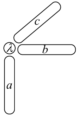
We will only consider symmetric tensors in this article. A tensor $\mathcal{A}$ is symmetric if $\mathcal{A}_{i_{1}\ldots i_{d}}=\mathcal{A}_{\pi(i_{1}\ldots i_{d})}$, where $\pi(i_{1}\ldots i_{d})$ is any permutation of the indices $i_{1}\ldots i_{d}$. A rank-1 symmetric $d$-way tensor $\mathcal{A}$ is then given by the $d$-times repeated outer product $\mathcal{A}=\lambda\,a\circ a\circ\ldots\circ a\triangleq\lambda a^{d}$. The vectorization of a tensor $\mathcal{A}$, denoted $\operatorname{vec}{(\mathcal{A})}\in\mathbb{R}^{n_{1}\cdots n_{d}}$, is the vector obtained from taking all indices together into one mode. This implies that for a symmetrical rank-1 tensor $\mathcal{A}$, its vectorization is

$$\operatorname{vec}{(\mathcal{A})}\;=\;\lambda\,a\otimes a\otimes\ldots\otimes a\;=\;\lambda\,a\textsuperscript{\textcircled{$d$}},$$

where we have introduced the shorthand notation $a\textsuperscript{\textcircled{$d$}}$ for the $d$-times repeated Kronecker product $\otimes$. Using the vectorization operation we can write (1) as

$$\operatorname{vec}{(\mathcal{A})}\;=\;\lambda_{1}\,x_{1}\textsuperscript{\textcircled{$d$}}+\ldots+\lambda_{R}\,x_{R}\textsuperscript{\textcircled{$d$}},$$

(2)

or equivalently as

$$\operatorname{vec}{(\mathcal{A})}\;=\;X\;l,$$

where $X$ is the matrix that is formed by the concatenation of all the $x_{1}\textsuperscript{\textcircled{$d$}},\ldots,x_{R}\textsuperscript{\textcircled{$d$}}$ vectors and $l\in\mathbb{R}^{R}$. In other words, the vectorization of a symmetric tensor $\mathcal{A}$ lives in the range of $X$, which is spanned by vectors $x_{i}\textsuperscript{\textcircled{$d$}}$. This requirement puts the known constraint [5] on the rank of $X$

$$\textrm{rank}(X)\leq R_{\textrm{max}}\triangleq{d+n-1\choose n-1},$$

for which we give a short proof in Lemma 1. The inverse vectorization operation $\operatorname{unvec}$ reshapes a vectorized tensor back into a tensor $\mathcal{A}=\operatorname{unvec}{(\operatorname{vec}{(\mathcal{A})})}$.

We now demonstrate the STEROID algorithm that decomposes a symmetric tensor into a real finite sum of symmetric rank-one outer factors by means of a 4-way tensor. Later on, we then show that STEROID is applicable to any tensor order via an innovative tensor embedding technique. The first step in the STEROID algorithm is to reshape the (4-way) symmetric $\mathcal{A}\in\mathbb{R}^{n\times n\times n\times n}$ into a 2-way symmetric matrix $A^{(n^{2}\times n^{2})}$, where the bracketed superscript indicates the dimensions. The symmetry of the reshaped $A$ follows trivially from the symmetry of $\mathcal{A}$. Now the eigendecomposition of $A$ can be computed, which allows us to write

$$A\;=\;\sum_{i=1}^{n^{2}}\,\lambda_{i}\,v_{i}\circ v_{i}\;=\;\sum_{i=1}^{n^{2}}\,\lambda_{i}\,v_{i}\,v_{i}^{T}.$$

(3)

The symmetry of $A$ implies that the eigenvalues $\lambda_{i}$ are real and the eigenvectors $v_{i}$ will be orthonormal. Both eigenvalues and eigenvectors can be computed by for example the symmetric QR algorithm or the divide-and-conquer method [11]. Each of these eigenvectors $v_{i}$ can now be reshaped into another 2-way symmetric matrix $\bar{v}_{i}^{(n\times n)}$. It is readily shown that the $\bar{v}_{i}$ vectors are also symmetric. Specifically, the symmetry of $A$ implies that we can write

$$A\,P\;=\;A,$$

(4)

where $P$ is any permutation matrix that permutes the indices $i_{\frac{d}{2}+1}\ldots i_{d}$. Using the eigendecomposition of $A$, we can rewrite (4) as

$$(\lambda_{1}\,v_{1}v_{1}^{T}+\ldots+\lambda_{n^{2}}\,v_{n^{2}}v_{n^{2}}^{T})\,P\;=\;(\lambda_{1}\,v_{1}v_{1}^{T}+\ldots+\lambda_{n^{2}}\,v_{n^{2}}v_{n^{2}}^{T}).$$

(5)

Left-multiplying (5) with the eigenvector $v_{i}^{T}\,(i=1,\ldots,n^{2})$ of the $i$th term, assuming $\lambda_{i}\neq 0$, we obtain

	$\displaystyle v_{i}^{T}\,(\lambda_{1}\,v_{1}v_{1}^{T}+\ldots+\lambda_{n^{2}}\,v_{n^{2}}v_{n^{2}}^{T})\,P$	$\displaystyle=v_{i}^{T}\,(\lambda_{1}\,v_{1}v_{1}^{T}+\ldots+\lambda_{n^{2}}\,v_{n^{2}}v_{n^{2}}^{T}),$
	$\displaystyle\Leftrightarrow\lambda_{i}v_{i}^{T}P$	$\displaystyle=\lambda_{i}v_{i}^{T},$
	$\displaystyle\Leftrightarrow v_{i}^{T}P$	$\displaystyle=v_{i}^{T},$

which implies that any of the eigenvectors $v_{i}\,(i=1,\ldots,n^{2})$ and consequently their reshaped $\bar{v}_{i}$ inhibit the same symmetry as $A$. The eigendecomposition of each of the symmetric $\bar{v}_{i}$’s can now also be computed. For example, $\bar{v}_{1}$ can then be written as

$$\bar{v}_{1}\;=\;\sum_{i=1}^{n}\,\lambda_{1i}\,v_{1i}\circ v_{1i},$$

where the $v_{1i}$’s are again orthogonal due to the symmetry of $\bar{v}_{1}$. The whole procedure of repeated eigendecompositions of the reshaped eigenvectors for a $d=4,n=2$ example is depicted in Figure 2.

Referring to Figure 2, we now take the $k$th term of (3) and vectorize it to obtain

$$\operatorname{vec}{(\lambda_{k}v_{k}v_{k}^{T})}=\lambda_{k}v_{k}\textsuperscript{\textcircled{2}}.$$

Substitution of $v_{k}$ by its eigendecomposition allows us to write

	$\displaystyle\lambda_{k}v_{k}\textsuperscript{\textcircled{2}}=$	$\displaystyle\lambda_{k}\left(\lambda_{k1}v_{k1}\textsuperscript{\textcircled{2}}+\lambda_{k2}v_{k2}\textsuperscript{\textcircled{2}}\right)\otimes\left(\lambda_{k1}v_{k1}\textsuperscript{\textcircled{2}}+\lambda_{k2}v_{k2}\textsuperscript{\textcircled{2}}\right)$
	$\displaystyle=$	$\displaystyle\underbrace{\lambda_{k}\lambda_{k1}^{2}v_{k1}\textsuperscript{\textcircled{4}}+\lambda_{k}\lambda_{k2}^{2}v_{k2}\textsuperscript{\textcircled{4}}}_{h_{k}}+\underbrace{\lambda_{k}\lambda_{k1}\lambda_{k2}\left(v_{k1}\textsuperscript{\textcircled{2}}\otimes v_{k2}\textsuperscript{\textcircled{2}}+v_{k2}\textsuperscript{\textcircled{2}}\otimes v_{k1}\textsuperscript{\textcircled{2}}\right)}_{t_{k}}$		(6)

where $h_{k}$ denotes the “head” part containing the pure powers $v_{k1}\textsuperscript{\textcircled{4}},v_{k2}\textsuperscript{\textcircled{4}}$ of $v_{k1}$ and $v_{k2}$, respectively, whereas $t_{k}$ denotes the “tail” holding the sum of cross terms. Defining the head tensor $\mathcal{H}=\operatorname{unvec}{(\sum_{k}h_{k})}$ and the tail tensor $\mathcal{T}=\operatorname{unvec}{(\sum_{k}t_{k})}$, it can be deduced that $\mathcal{T}=\mathcal{A}-\mathcal{H}$ must also be 4-way symmetric since $\mathcal{A}$ and $\mathcal{H}$ are so. As we will explain further on, the symmetry of the tail tensor $\mathcal{T}$ is crucial, since it is possible that repeated eigendecompositions of the reshapings of $\mathcal{T}$ are also necessary in order to compute additional pure power vectors of the STEROID. The objective now is to write $\textrm{vec}(\mathcal{A})$ as a linear combination

$$\operatorname{vec}{(\mathcal{A})}\;=\;l_{1}x_{1}\textsuperscript{\textcircled{4}}+\ldots+l_{R}x_{R}\textsuperscript{\textcircled{4}}.$$

Good candidates for the $x_{i}\textsuperscript{\textcircled{4}}$ vectors are the pure powers that span the head part in (6). No pure power vectors should be considered that come from an eigenvector with corresponding zero eigenvalue $\lambda_{k}$. Since each of the $x_{i}$’s is an eigenvector of a symmetric matrix, it also follows that $||x_{i}\textsuperscript{\textcircled{4}}||_{F}=1$. Checking whether a decomposition as in (2) exists is done by computing the residual of the following least-squares problem

$$\hat{l}\;=\;\underset{l}{\operatorname{argmin}}\;||\operatorname{vec}{(\mathcal{A})}-X\,l\,||_{F},$$

(7)

where $X$ is the matrix obtained from the concatenation of all the obtained pure power vectors $x_{i}\textsuperscript{\textcircled{4}}$. It is possible at this step to solve (7) with additional constraints. For example, if only positive $l_{i}$’s are required then one could use a reflective Newton method as described in [4]. A sparse solution $\hat{l}$ with as few nonzero $l_{i}$’s as possible can be computed using L1-regularization [28]. The particular repeated Kronecker product structure for each column of $X$ results in the following upper bound on its rank.

Lemma 1 tells us that vec($\mathcal{A}$) of a symmetric tensor $\mathcal{A}$ lives in a $R_{\textrm{max}}$-dimensional vector space. Therefore, instead of computing the STEROID, one could randomly generate $R_{\textrm{max}}$ linearly independent vectors, construct their corresponding $X$ matrix and decompose vec($\mathcal{A}$) along this basis. However, a random basis will most likely result in a decomposition with $R_{\textrm{max}}$ nonzero terms, while the STEROID results in a more compact decomposition, as is illustrated in the following example.

From Lemma 1 we learn two things. First, it is possible that not enough pure power vectors are computed to solve the least-squares problem (7). In this case the residual $||\operatorname{vec}{(\mathcal{A})}-X\,\hat{l}||_{F}$ will not be satisfactory and the same procedure of reshapings and eigendecompositions should be applied to the tail tensor $\mathcal{T}$. This will produce additional pure powers that can be used to extend $X$, upon which one can solve the least-squares problem (7) again. Further iterations on the resulting tail tensor can be applied until a satisfactory residual is obtained. The second thing we learn is that it is also possible that $X$ becomes singular as soon as it has more than ${d+n-1\choose n-1}$ columns. In this case it is recommended to regularize the least-squares problem such that the obtained solution is not sensitive to perturbations of the tensor $\mathcal{A}$. This can be done by for example computing the minimum norm solution of (7). The whole STEROID algorithm for tensors with $d=2^{k}\,(k\in\mathbb{N})$ is summarized in pseudo-code in Algorithm 2.1. Matlab/Octave implementations can be freely downloaded from https://github.com/kbatseli/STEROID.

Algorithm 2.1.

STEROID algorithm
Input: symmetric $d$-way tensor $\mathcal{A}$ with $d=2^{k},k\in\mathbb{N}$, tolerance $\tau$
Output: pure power vectors $x_{i}$, $\hat{l}$  $\bar{\mathcal{A}}\leftarrow$ reshape $\mathcal{A}$ into a $n^{d/2}\times n^{d/2}$ matrix  $V_{1},D_{1}\leftarrow$ eig($\bar{\mathcal{A}}$)  for all eigenvectors $V_{1}(:,i)$ with $\lambda_{i}\neq 0$ do   recursively reshape $V_{1}(:,i)$ and compute its eigendecomposition  end for  compute head tensor $\mathcal{H}$ from recursive eigendecompositions of $\mathcal{A}$  $\mathcal{T}\leftarrow\mathcal{A}$  collect all pure powers into $X$  solve least-squares problem $\hat{l}=\underset{l}{\operatorname{argmin}}\;||\operatorname{vec}{(\mathcal{A})}-X\,l||_{F}$  while $||\operatorname{vec}{(\mathcal{A})}-X\,\hat{l}||_{2}>\tau$ AND $\textrm{rank}\,(X)<R_{\textrm{max}}$ do   $\mathcal{T}\leftarrow\mathcal{T}-\mathcal{H}$   add additional pure powers to $X$ by recursive eigendecompositions of $\mathcal{T}$   compute new head tensor $\mathcal{H}$ from recursive eigendecompositions of $\mathcal{T}$   extend $X$ with additional pure powers   solve least-squares problem $\hat{l}=\underset{l}{\operatorname{argmin}}\;||\operatorname{vec}{(\mathcal{A})}-X\,l||_{F}$  end while

Every matrix from which an eigendecomposition is computed in Algorithm 2.1 is symmetric. This implies that the computed eigenvalues are up to a sign equal to the singular values. Hence the same kind of tolerance as for the singular values can be used to determine whether any of the $\lambda_{i}$’s are numerically zero [11]. Note that a user-defined tolerance $\tau$ is required to check whether additional iterations on the tail tensor $\mathcal{T}$ are required.

The computational complexity of the method is dominated by the very first eigendecomposition of the $n^{d/2}\times n^{d/2}$ matrix $A$ and by solving the least-squares problem (7). The first eigendecomposition requires a tridiagonalization of $A$, which requires $8/3\,n^{3d/2}$ flops and dominates the cost. For the actual diagonalization, QR iterations or the divide-and-conquer method can be used. The matrix $X$ in the least-squares problem also determines the computational cost. Its number of rows is $n^{d}$ and we can assume its number of columns to be $R_{\textrm{max}}$. Solving the least-squares problem with the SVD of $X$ then sets the maximal computational complexity to $2R_{\textrm{max}}^{2}(n^{d}-R_{\textrm{max}}/3)$. In Section 3 we discuss two ways in which the size of the least-squares problem can be significantly reduced by exploiting the symmetry of $\mathcal{A}$ and the structure of $X$.

It is clear that the STEROID algorithm presented in Algorithm 2.1 only works for symmetric tensors for which the order is a power of 2. Indeed, this is a necessary requirement such that the recursive reshapings in the algorithm always lead to a square symmetric matrix. Fortunately, by employing an embedding procedure one can compute the STEROID of a symmetric tensor $\mathcal{A}$ of any order. We now discuss this embedding procedure in the next section.

The embedding procedure presented in this section allows us to compute the STEROID for a symmetric tensor of an arbitrary order. Algorithm 2.1 relies on the reshaping of the tensor into a square matrix and therefore the order of the tensor should be divisible by two. If the order $d$ is odd, then one can embed the tensor into a symmetric tensor of order $d+1$, reshape it again into a square matrix and continue Algorithm 2.1. We now illustrate the embedding procedure with a 3-way symmetric tensor $\mathcal{A}$ of dimension 2 into a symmetric tensor $\mathcal{B}$ of order 4. Since $\mathcal{A}$ is symmetric, it only has 4 distinct entries, viz. $\mathcal{A}_{111},\mathcal{A}_{211}(=\mathcal{A}_{121}=\mathcal{A}_{112}),\mathcal{A}_{221}(=\mathcal{A}_{212}=\mathcal{A}_{122}),\mathcal{A}_{222}$. The idea now is to consider $\mathcal{A}$ as the frontal “slice” of $\mathcal{B}$ in the following straightforward manner

	$\displaystyle\mathcal{A}_{111}$	$\displaystyle\Rightarrow\mathcal{B}_{1111},$
	$\displaystyle\mathcal{A}_{211}$	$\displaystyle\Rightarrow\mathcal{B}_{2111},$
	$\displaystyle\mathcal{A}_{221}$	$\displaystyle\Rightarrow\mathcal{B}_{2211},$
	$\displaystyle\mathcal{A}_{222}$	$\displaystyle\Rightarrow\mathcal{B}_{2221}.$

In order to make sure that $\mathcal{B}$ is symmetric, one needs to enforce the following equalities

	$\displaystyle\mathcal{B}_{2111}$	$\displaystyle=\mathcal{B}_{1211}=\mathcal{B}_{1121}=\mathcal{B}_{1112},$
	$\displaystyle\mathcal{B}_{2211}$	$\displaystyle=\mathcal{B}_{2121}=\mathcal{B}_{2112}=\mathcal{B}_{1221}=\mathcal{B}_{1212}=\mathcal{B}_{1122},$
	$\displaystyle\mathcal{B}_{2221}$	$\displaystyle=\mathcal{B}_{2212}=\mathcal{B}_{2122}=\mathcal{B}_{1222}.$

All other entries of $\mathcal{B}$, in this example $\mathcal{B}_{2222}$, can be set to zero. We now have a symmetric $\mathcal{B}$ with $\mathcal{B}_{i_{1}i_{2}i_{3}1}=\mathcal{A}_{i_{1}i_{2}i_{3}}$. The general embedding algorithm is presented in pseudo-code in Algorithm 2.2.

Algorithm 2.2.

symmetric tensor embedding algorithm
Input: symmetric $d$-way cubical tensor $\mathcal{A}$ with $d$ an odd number
Output: symmetric $d+1$-way cubical tensor $\mathcal{B}$ with $\mathcal{B}_{i_{1}\ldots i_{d}1}=\mathcal{A}_{i_{1}\ldots i_{d}}$.  initialize $\mathcal{B}$ with zeros  for all nonzero $\mathcal{A}_{i_{1}\ldots i_{d}}$ do   for all permutations $\pi(i_{1}\ldots i_{d}1)$ do    $\mathcal{B}_{\pi(i_{1}\ldots i_{d}1)}\leftarrow\mathcal{A}_{i_{1}\ldots i_{d}}$   end for  end for


Using Algorithm 2.2, it now becomes possible to adjust the STEROID algorithm such that it works for a symmetric tensor of any order. Indeed, if the order $d$ is odd, then application of Algorithm 2.2 guarantees that the new symmetric tensor can be reshaped into a square matrix. Similarly, the obtained eigenvectors can be embedded if necessary. The following example illustrates the STEROID algorithm with embedding.

The symmetry of $\mathcal{A}$ implies that many rows of $X$ will be identical. In fact, only ${d+n-1\choose n-1}$ rows are unique due to Lemma 1. If $S$ is the row selection matrix that selects the ${d+n-1\choose n-1}$ unique rows from $X$ then (7) can be rewritten as the mathematically equivalent problem

$$\hat{l}\;=\;\underset{l}{\operatorname{argmin}}\;||S\,\operatorname{vec}{(\mathcal{A})}-S\,X\,l||_{F}.$$

(8)

The number of rows of $X$ are then reduced with a factor of

$$\gamma\triangleq\frac{n^{d}}{{d+n-1\choose n-1}}\;=\;\frac{n^{d}\,(n-1)!}{(d+n-1)\cdots(d+1)},$$

which grows exponential in $d$. Figure 3 demonstrates the reduction factor $\gamma$ as a function of $n$ for different orders $d$. It can be seen that the reduction in number of rows first increases exponentially for small $n$ and then quickly ‘saturates’ to an almost constant factor.

Although massive savings can be achieved by exploiting the symmetry of $\mathcal{A}$, $S\,X$ still has ${d+n-1\choose n-1}=d^{n-1}/(n-1)!+O(d^{n-2})$ rows, which grows exponential in $n$. This implies that even for moderate $d$, (7) will quickly become infeasible for increasing $n$. In the next section we discuss how the size of the least-squares problem can be further reduced by exploiting the particular structure of $X$. This will come, however, at the cost of a squared condition number when solving (7).

The matrix $X$ is typically very thin, with much more rows than columns. We assume in this section that $X$ is of full column rank. One straightforward way then to reduce the size of the matrix is to left-multiply with $X^{T}$ to obtain

$$X^{T}\,X\,l\;=\;X^{T}\,\textrm{vec}(\mathcal{A}).$$

Since $X$ is of full column rank, $l$ will be unique and $X^{T}\,X$ will be symmetric and positive definite. This means that in addition to getting rid of the $n^{d}$ rows, only half of the entries of $X^{T}\,X$ need to be stored. This comes at the cost of a squared condition number $\kappa(X^{T}\,X)=\kappa(X)^{2}$, where $\kappa(X)$ denotes the condition number of the matrix $X$.

The matrix $X^{T}\,X$ can also be constructed without explicitly constructing $X$, what is to be avoided in the first place. Indeed, each column of $X$ is a repeated Kronecker product of a pure power vector $x_{i}\textsuperscript{\textcircled{$d$}}$. Each element of $X^{T}\,X$ is therefore an inner product $x_{i}\textsuperscript{\textcircled{$d$}}\,x_{j}\textsuperscript{\textcircled{$d$}}$, which can be rewritten as

$$x_{i}^{T}x_{j}\otimes x_{i}^{T}x_{j}\otimes\ldots\otimes x_{i}^{T}x_{j}\;=\;(x_{i}^{T}x_{j})^{d}.$$

This allows us to construct $X^{T}\,X$ without the explicit construction of $X$ as described in the following lemma.

We first demonstrate the STEROID on a simple symmetric 3rd-order tensor

$$\mathcal{A}_{111}=24,\mathcal{A}_{211}=18,\mathcal{A}_{221}=12,\mathcal{A}_{222}=6,$$

which we first need to extend to a 4th-order symmetrical cubical tensor $\mathcal{B}$ using Algorithm 2.2. The next step of the STEROID algorithm is to reshape $\mathcal{B}$ into the following $4\times 4$ symmetric matrix

$$B\;=\;\begin{pmatrix}24&18&18&12\\ 18&12&12&6\\ 18&12&12&6\\ 12&6&6&0\end{pmatrix}$$

and compute its eigendecomposition

$$B\;=\;V\begin{pmatrix}-5.3939&0&0&0\\ 0&-6.29\times 10^{-15}&0&0\\ 0&0&2.64\times 10^{-15}&0\\ 0&0&0&53.3939\\ \end{pmatrix}\,V^{T}.$$

Since $B$ has 2 eigenvalues that are numerically zero, we only need to proceed with the eigenvectors $V(:,1)$ and $V(:,4)$, where we used MATLAB notation to denote the first and fourth columns of $V$. Reshaping both $V(:,1)$ and $V(:,4)$ into a symmetric $2\times 2$ matrix and computing their eigendecomposition results in the following 4 pure power vectors

$$x_{1}=\begin{pmatrix}-0.9939\\ 0.1103\end{pmatrix},x_{2}=\begin{pmatrix}-0.1103\\ -0.9939\end{pmatrix},x_{3}=\begin{pmatrix}-0.8396\\ -0.5431\end{pmatrix},x_{4}=\begin{pmatrix}0.5431\\ -0.8396\end{pmatrix}.$$

Solving the least-squares problem

$$\hat{l}\;=\;\underset{l}{\operatorname{argmin}}\;||\operatorname{vec}{(\mathcal{A})}-\begin{pmatrix}x_{1}\textsuperscript{\textcircled{3}}&x_{2}\textsuperscript{\textcircled{3}}&x_{3}\textsuperscript{\textcircled{3}}&x_{4}\textsuperscript{\textcircled{3}}\end{pmatrix}\,l||_{F},$$

results in

$$\hat{l}\;=\;\begin{pmatrix}3.9934\\ 0.6922\\ -46.79\\ 1.3916\end{pmatrix},$$

with a residual of $1.8546\times 10^{-14}$. Observe that the total number of terms in the computed decomposition equals the upper bound ${3+2-1\choose 2-1}=4$. The total run time to compute the decomposition was $7.5\times 10^{-4}$ seconds.

Another interesting example, that can be found in [5], is the symmetric tensor defined by

$$\mathcal{A}_{111}=-1,\mathcal{A}_{221}=1.$$

The STEROID algorithm computes the following decomposition

$$\mathcal{A}\;=\;-2\begin{pmatrix}1\\ 0\end{pmatrix}^{\textsuperscript{\textcircled{3}}}-1.4142\begin{pmatrix}-0.7071\\ 0.7071\end{pmatrix}^{\textsuperscript{\textcircled{3}}}+1.4142\begin{pmatrix}0.7071\\ 0.7071\end{pmatrix}^{\textsuperscript{\textcircled{3}}}$$

in $0.0012$ seconds. This is the same decomposition as given in [5].

Consider a random symmetric tensor $\mathcal{A}\in\mathbb{R}^{7\times 7\times 7\times 7}$ with integer entries between 24 and 100. The STEROID algorithm returns 196 pure power vectors. The rank of $X$ is upper bounded by ${4+7-1\choose 7-1}=210$ and not surprisingly we have a residual of $70.2320$, which indicates that additional pure power vectors are required. Running Algorithm 2.1 on the tail tensor $\mathcal{T}$ returns an additional 189 pure power vectors. Solving the least-squares problem (7) with all 385 pure power vectors results in a residual of $1.49\times 10^{-11}$ and 167 nonzero entries in $l$. The upper bound of 210 on the rank of $X$, together with the set of 385 pure power vectors implies that there is distinct non-uniqueness in the decomposition.

For this numerical experiment six random symmetric tensors with dimension $n=5$ and orders $d=3$ up to $d=8$ were generated. Columns two and three of Table 1 list the total number of computed eigendecompositions and the total number of required embeddings for each value of $d$ in the STEROID computation. Columns four and five list the total run times in seconds for computing all eigendecompositions and doing the tensor embeddings. The rightmost column lists the total time required to compute the pure power $x_{i}$ vectors of the STEROID and is the sum of the entries in the fourth and fifth column. From Table 1 it can be seen that, unless the order is a power of two, the main contribution in the total time required to compute the pure power vectors comes from the embedding procedure. The 35 embeddings for $d=6$ take about half the amount of time as the 31 embedding for $d=5$. This is explained by the fact that $d=5$ requires 1 embedding from order 5 to 6 and 30 embeddings from order 3 to 4, while for $d=6$ there are 35 embeddings from order 3 to 4. Embedding a symmetric tensor from order 5 to order 6 is a much more time-consuming process than from order 3 to 4. The largest run time is observed for $d=7$, which requires only 1 embedding from order 7 to order 8.

Once all $x_{i}$ vectors are computed, we solve the least-squares problem (7) in three different ways: original (no reduction of the $X$ matrix), symmetry (exploiting the symmetry of $\mathcal{A}$), $X^{T}X$ (computes $X^{T}X$ using Lemma 2). Table 2 lists the residuals $||\mathcal{A}-X\hat{l}||_{F}$ and total run times in seconds for each of the three methods. The residuals for the $X^{T}X$ method are only slightly worse than the other two methods due to the squared condition number. This implies that the condition numbers of $X$ were relatively small. The difference in run time is more pronounced for higher orders. Most apparent is the saving with a factor of 6942 in run time between the original and symmetry exploiting methods when $d=8$. Exploiting the symmetry reduces the total number of rows of $X$ from $5^{8}=390625$ down to ${8+5-1\choose 5-1}=495$. This reduces $X$ to a $495\times 5550$ matrix of rank 495. Using the $X^{T}\,X$ method when $d=8$ reduces the run time with a factor 1174 but is clearly not as good as exploiting the symmetry. The reason for this difference lies in the fact that 5550 pure power vectors are computed and therefore $X^{T}\,X$ is a $5550\times 5550$ matrix, compared to the $495\times 5550$ matrix when symmetry is exploited.

In this numerical experiment, we apply the Jacobi [12], Regalia’s iterative symmetric tensor approximation algorithm [22] and the CANDECOMP-algorithm of the Tensorlab toolbox [27] to the symmetric tensors of Experiment 3. The Matlab implementation of the Jacobi algorithm was provided by Dr. Mariya Ishteva. This Jacobi method implementation only works for 3rd-order tensors. We implemented Regalia’s iterative algorithm and confirmed its results with the numerical experiments described in [22]. The Tensorlab toolbox is freely available. For a given multilinear rank $r$, the Jacobi and Regalia’s method return an orthogonal $n\times r$ matrix U and symmetric tensor core $\mathcal{S}\in\mathbb{R}^{n\times\ldots\times n}$ that minimize $||\mathcal{A}-\mathcal{S}\times_{1}U\times_{2}\cdots\times_{d}U||_{F}$. The maximal number of columns of $U$ is therefore limited to $n$. This implies that for a fully dense 3rd-order core tensor $\mathcal{S}$ one will have $1,4,10,20,35$ respective number of terms in the decomposition for $r=1,2,3,4,5$. Table 3 lists the total number of required iterations, the residual and total run time for the Jacobi method applied for all possible values of $r$. The initial orthogonal matrices to start the iterations were obtained from applying a QR orthogonalization on a random $n\times r$ matrix. The full Tucker decomposition is obtained for $r=5$ and consists of 32 nonsymmetric and 3 symmetric terms. In contrast, the STEROID consists of 50 symmetric terms and is obtained more than 3 times faster when symmetry is exploited.

Regalia’s iterative method is not limited to 3rd-order tensors and is therefore applied to all symmetric tensors of Experiment 3. Since we are interested in a full decomposition we set $r=5$ and therefore obtain ${3+5-1\choose 5-1},\ldots,{8+5-1\choose 5-1}$ terms for every respective decomposition. The initial orthogonal matrices to start the iterations were obtained from applying a QR orthogonalization on a random $n\times 5$ matrix. Table 4 lists the total number of required iterations, the residual and total run time for each symmetric tensor from Experiment 3. Iterations were stopped when the difference in consecutive orthogonal vectors over 2 iterations was smaller than $1\text{\times}{10}^{-10}$. An additional parameter $\gamma$ to ensure monotonic convergence was set to $20$. For $d=8$, the algorithm failed to finish due to a lack of sufficient memory. Compared to the symmetry exploiting STEROID algorithm, the total run time of Regalia’s iterative method is up to 35 times slower.

Finally, the CANDECOMP-algorithm from Tensorlab is applied to all symmetric tensors of Experiment 3. This algorithm allows each rank-1 term to be symmetric as well. In Table 5 the total number of computed terms, the residual and total run time in seconds are listed. As with Regalia’s iterative method, for $d=8$ the algorithm also fails due to the intermediate result being too large. Since we are interested in a full decomposition we set the total number of desired rank-1 terms equal to the number of terms obtained from the STEROID. This does surprisingly not result in small residuals for the CANDECOMP-algorithm. The total run time is highly variable over the different orders and for the $d=6$ case 4 times slower compared to the symmetry exploiting STEROID algorithm.

References

- [1] K. Batselier, H. Liu, and N. Wong, A constructive algorithm for decomposing a tensor into a finite sum of orthonormal rank-1 terms, ArXiv e-prints, (2014).
- [2] J. Brachat, P. Comon, B. Mourrain, and E. P. Tsigaridas, Symmetric tensor decomposition, Linear Algebra Appl., 433 (2010), pp. 1851–1872.
- [3] J.D. Carroll and J.-J. Chang, Analysis of individual differences in multidimensional scaling via an n-way generalization of “Eckart-Young” decomposition, Psychometrika, 35 (1970), pp. 283–319.
- [4] T. Coleman and Y. Li, A reflective newton method for minimizing a quadratic function subject to bounds on some of the variables, SIAM J. Optimiz., 6 (1996), pp. 1040–1058.
- [5] P. Comon, G. Golub, L.-H. Lim, and B. Mourrain, Symmetric tensors and symmetric tensor rank., SIAM J. Matrix Anal. Appl., 30 (2008), pp. 1254 – 1279.
- [6] P. Comon and M. Rajih, Blind identification of under-determined mixtures based on the characteristic function, Signal Processing, 86 (2006), pp. 2271 – 2281. Special Section: Signal Processing in {UWB} Communications.
- [7] L. De Lathauwer, J. Castaing, and J. Cardoso, Fourth-order cumulant-based blind identification of underdetermined mixtures, IEEE T. Signal Proces., 55 (2007), pp. 2965–2973.
- [8] P. Dreesen, M. Ishteva, and J. Schoukens, Decoupling multivariate polynomials using first-order information and tensor decompositions, SIAM J. Matrix Anal. Appl., (2015). Accepted for publication (preprint arXiv:1410.4060 [math.NA]).
- [9] A. Ferreol, L. Albera, and P. Chevalier, Fourth-order blind identification of underdetermined mixtures of sources (FOBIUM), IEEE T. Signal Proces., 53 (2005), pp. 1640–1653.
- [10] F. Giri and E.-W. Bai, Block-oriented nonlinear system identification, vol. 1, Springer, 2010.
- [11] G. H. Golub and C. F. Van Loan, Matrix Computations, The Johns Hopkins University Press, 3rd ed., Oct. 1996.
- [12] M. Ishteva, P.-A. Absil, and P. Van Dooren, Jacobi algorithm for the best low multilinear rank approximation of symmetric tensors, SIAM J. Matrix Anal. Appl., 34 (2013), pp. 651–672.
- [13] E. Kofidis and P. A. Regalia, On the best rank-1 approximation of higher-order supersymmetric tensors, SIAM J. Matrix Anal. Appl., 23 (2002), pp. 863–884.
- [14] T.G. Kolda, Orthogonal tensor decompositions, SIAM J. Matrix Anal. Appl., 23 (2001), pp. 243–255.
- [15] T.G. Kolda and B.W. Bader, Tensor decompositions and applications, SIAM Rev., 51 (2009), pp. 455–500.
- [16] T. G. Kolda and J. R. Mayo, Shifted power method for computing tensor eigenpairs, SIAM J. Matrix Anal. Appl., 32 (2011), pp. 1095–1124.
- [17] , An adaptive shifted power method for computing generalized tensor eigenpairs, SIAM J. Matrix Anal. Appl., 35 (2014), pp. 1563–1581.
- [18] JM Landsberg, Tensors: geometry and applications, vol. 128, American Mathematical Society, 2012.
- [19] I. Oseledets, Tensor-train decomposition, SIAM J. Sci. Comput., 33 (2011), pp. 2295–2317.
- [20] Johan Paduart, Lieve Lauwers, Jan Swevers, Kris Smolders, Johan Schoukens, and Rik Pintelon, Identification of nonlinear systems using polynomial nonlinear state space models, Automatica, 46 (2010), pp. 647–656.
- [21] MATLAB R2012a, The Mathworks Inc., 2012. Natick, Massachusetts.
- [22] P.A Regalia, Monotonically convergent algorithms for symmetric tensor approximation, Linear Algebra Appl., 438 (2013), pp. 875 – 890.
- [23] P.A. Regalia and E. Kofidis, The higher-order power method revisited: convergence proofs and effective initialization, in Acoustics, Speech, and Signal Processing, 2000. ICASSP ’00. Proceedings. 2000 IEEE International Conference on, vol. 5, 2000, pp. 2709–2712 vol.5.
- [24] J. Salmi, A. Richter, and V. Koivunen, Sequential unfolding svd for low rank orthogonal tensor approximation, in Signals, Systems and Computers, 2008 42nd Asilomar Conference on, Oct 2008, pp. 1713–1717.
- [25] B. Savas and L.-H. Lim, Quasi-newton methods on grassmannians and multilinear approximations of tensors, SIAM J. Sci. Comput., 32 (2010), pp. 3352–3393.
- [26] M. Schoukens and Y. Rolain, Cross-term elimination in parallel wiener systems using a linear input transformation, IEEE T. Instrum. Meas., 61 (2012), pp. 845–847.
- [27] L. Sorber, M. Van Barel, and L. de Lathauwer, Tensorlab Version 2.0. Available online, January 2014.
- [28] R. Tibshirani, Regression shrinkage and selection via the lasso, J. Roy. Stat. Soc. B, 58 (1994), pp. 267–288.
- [29] K. Tiels and J. Schoukens, From coupled to decoupled polynomial representations in parallel wiener-hammerstein models, in Decision and Control (CDC), 2013 IEEE 52nd Annual Conference on, IEEE, 2013, pp. 4937–4942.
- [30] K. Usevich, Decomposing multivariate polynomials with structured low-rank matrix completion, in Proc. 21st MTNS, July 2014, pp. 1826–1833.
- [31] A. Van Mulders, J. Schoukens, and L. Vanbeylen, Identification of systems with localised nonlinearity: from state-space to block-structured models, Automatica, 49 (2013), pp. 1392–1396.