Uncertainty Quantification for Integrated Circuits: Stochastic Spectral Methods

Univariate gPC. For $\xi_{k}\in\Omega_{k}\subseteq\mathbb{R}$, one can construct a set of polynomial functions subject to the orthonormal condition:

where $\langle,\rangle$ denotes the inner product; $\delta_{\gamma,\nu}$ is a Delta function; integers $\gamma$ and $\nu$ are the degrees of $\xi_{k}$ in polynomials $\phi^{k}_{\gamma}({\xi_{k}})$ and $\phi^{k}_{\nu}({\xi_{k}})$, respectively. Given ${\rho_{k}}({\xi_{k}})$ and $\Omega_{k}$, one can utilize a three-term recurrence relation to construct such orthonormal polynomials [48]. Some univariate gPC basis functions are listed in Table I as a demonstration. It is worth noting that: 1) the univariate gPC basis functions are not limited to the cases listed in Table I; 2) when $\xi_{k}$ is a Gaussian variable, its gPC simplifies to the Hermite polynomial chaos [30].

Multivariate gPC. When the components of $\vec{\xi}$ are assumed mutually independent, the multivariate gPC can be constructed based on the univariate gPC of each $\xi_{k}$. Given an index vector $\vec{\alpha}=[\alpha_{1},\cdots,\alpha_{d}]\in\mathbb{N}^{d}$, the corresponding multivariate gPC is constructed as

The obtained multivariate gPC is orthonormal, i.e.,

Note that $H_{\vec{\alpha}}({\vec{\xi}})$ is the product of different types of univariate gPC bases when $\xi_{k}$’s have different density functions.

If $\vec{x}({\vec{\xi}},t)$ is a 2nd-order stochastic process (i.e., $\vec{x}({\vec{\xi}},t)$ has a bounded 2nd-order moment), we can approximate it by a finite-term gPC expansion

where $\hat{x}_{\vec{\alpha}}(t)\in\mathbb{R}^{n}$ denotes the gPC coefficient with index ${\vec{\alpha}}$, and ${\cal P}$ is a set containing some properly selected index vectors.

Given $p\in\mathbb{N}^{+}$, there are two popular choices for ${\cal P}$ [23]. In the tensor product method, one sets ${\cal P}=\{\vec{\alpha}|\;0\leq\alpha_{k}\leq p\}$, leading to a total of $(p+1)^{d}$ gPC bases. In order to reduce the total number of basis functions, the total degree scheme sets ${\cal P}=\{\vec{\alpha}|\;\alpha_{k}\in\mathbb{N},\;0\leq{\alpha_{1}}+\cdots+\alpha_{d}\leq p\}$, leading to

gPC bases in total. This total degree method is employed in our stochastic circuit simulator. There is a one-to-one correspondence between $k$ (with $1\leq k\leq K$) and the index vector $\vec{\alpha}$, thus for simplicity (5) is normally rewritten as

It is shown that gPC expansions converge exponentially for some analytical functions [25, 27, 29]. Such exponential convergence rates may not be observed in practical engineering problems, but gPC still converge very fast when the function of interest has a smooth dependence on $\vec{\xi}$. With gPC approximations, some statistical information (e.g., mean and variance) can be easily calculated due to the orthonormality of $H_{k}(\vec{\xi})$’s.

This section briefly reviews some numerical quadrature methods widely used in stochastic spectral methods.

1-D Case. When computing an integral with a quadrature method one typically uses the expression

when $g\left({\xi_{k}}\right)$ is a smooth function. The quadrature points ${\xi_{k}^{j}}$’s and weights $w_{k}^{j}$’s are chosen according to $\Omega_{k}$ and $\rho_{k}\left({\xi_{k}}\right)$. Two kinds of quadrature rules are widely used: Gauss quadrature [49] and Clenshaw-Curtis rules [50, 51]. With $\hat{n}$ points, Gauss quadrature rule produces exact results for all polynomials of degree $\leq 2\hat{n}-1$, and Clenshaw-Curtis gets exact results when the degree of $g(\xi_{k})$ is $\leq\hat{n}-1$. Clenshaw-Curtis scheme generates nested quadrature points and assumes that $\xi_{k}$ is uniformly distributed in a bounded domain.

Multi-dimensional Case. One can also evaluate a multidimensional integral in $\Omega\subseteq\mathbb{R}^{d}$ using the formula

where $\hat{N}$ is the total number of quadrature points, and $w^{j}$ is the weight corresponding to quadrature point $\vec{\xi}^{j}$. Given the 1-D quadrature points for each $\xi_{k}$, $\vec{\xi}^{j}$’s and $w^{j}$’s can be obtained for instance using a tensor-product rule or using sparse grids [52, 53]. With Smolyak’s algorithm, sparse grid technique uses much fewer quadrature points than the tensor-product rule, thus it is widely used to solve stochastic PDEs [31, 32, 33, 34]. In [31, 32, 33, 34] Smolyak’s algorithm produces nested sparse grids because all random parameters are assumed uniformly distributed (and thus Clenshaw-Curtis rule is used for all $\xi_{k}$’s). However, Smolyak’s algorithm generates non-nested sparse grids when non-nested 1-D quadrature points are used for some parameters (since many random parameters with non-uniform distributions may not be effectively handled by the Clenshaw-Curtis rule).

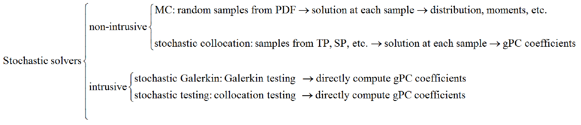
The main stochastic solvers are classified in Fig. 1. MC and stochastic collocation are both non-intrusive (or sampling-based) methods: they solve (1) as a deterministic problem at a set of samples. Their main difference lies in the sampling stage: MC randomly draws some samples based on $\rho(\vec{\xi})$, whereas stochastic collocation typically uses the points from a tensor-product or sparse-grid rule such that the gPC coefficients can be well reconstructed. Stochastic Galerkin and stochastic testing belong to the family of intrusive solvers: through solving a new coupled differential algebraic equation they directly compute the gPC coefficients. The former sets up the coupled equation by Galerkin testing, whereas the latter constructs a coupled equation via collocation testing.

The stochastic testing method needs to select $K$ testing points $\vec{\xi}_{1},\cdots,\vec{\xi}_{K}$. First, a quadrature scheme (e.g., tensor-product or sparse grid rule in Section II-C) is applied to generate $\hat{N}$ quadrature points $\vec{\xi}^{j}$’s in parameter space $\Omega$, which are called candidate nodes. Second, the $K$ most important candidate nodes are selected such that the transformation matrix $\textbf{V}\in\mathbb{R}^{K\times K}$, with its $(i,j)$ entry being

is invertible and well conditioned.

Define a vector function $\vec{H}(\vec{\xi}):=[H_{1}(\vec{\xi});\cdots;H_{K}(\vec{\xi})]$, then the testing points can be selected by Algorithm 1 [43]. Only a small portion of the candidate nodes are finally selected as the testing points.

Let $\hat{\textbf{x}}(t)=[\hat{x}^{1}(t);\cdots;\hat{x}^{K}(t)]$ denote the gPC coefficients, $\tilde{q}(\hat{\textbf{x}}(t),\vec{\xi})=\vec{q}({\tilde{x}({t,\vec{\xi}}),\vec{\xi}})$ and $\tilde{f}(\hat{\textbf{x}}(t),\vec{\xi})=\vec{f}({\tilde{x}({t,\vec{\xi}}),\vec{\xi}})$. Substituting $\tilde{x}(t,\vec{\xi})$ of (7) into (1) yields a residual function

Collocation Testing. Enforcing the residual function to zero at all testing points, stochastic testing generates the following coupled differential algebraic equation:

where the $k$-th blocks of $\textbf{q}(\hat{\textbf{x}}(t))$, $\textbf{f}(\hat{\textbf{x}}(t))$ and B are $\tilde{q}(\hat{\textbf{x}}(t),\vec{\xi}_{k})$, $\tilde{f}(\hat{\textbf{x}}(t),\vec{\xi}_{k})$ and $B$, respectively.

Numerical Solver. Stochastic testing is an intrusive solver: the gPC coefficients $\hat{\textbf{x}}(t)$ are directly computed by simulating (12), then the parameter-dependent current/voltage variables are obtained by gPC approximations. In transient analysis, the time step sizes can be selected adaptively according to the local truncation error (LTE) of (12) as done in commercial deterministic circuit simulators [17, 18]. Another desirable feature of stochastic testing is the decoupling procedure inside the intrusive solver. Assume that J is the Jacobian inside the Newton’s iteration when simulating (12) (as a DC problem or as a transient problem using numerical integration such as backward Euler). It is shown in [43] that J can be factored as

where ${\rm blkdiag}$ is the block diagonal operator, $\otimes$ is the Kronecker product operation, and $\textbf{I}_{n}\in\mathbb{R}^{n\times n}$ is an identity matrix. Matrix $J_{k}\in\mathbb{R}^{n\times n}$ can be treated as a Jacobian corresponding to (1) with $\vec{\xi}=\vec{\xi}_{k}$. Since the Vandermonde-like matrix V [as defined in (10)] can be easily inverted [54], the linear system solution inside each Newton’s iteration can be decoupled into $K$ small-size problems. Consequently, the overall computational cost scales linearly with $K$ [43].

Galerkin Testing. Applying Galerkin testing

for $k=1,\cdots,K$, stochastic Galerkin forms a coupled equation in the form of (12). Now the $k$-th blocks of $\textbf{q}(\hat{\textbf{x}}(t))$, $\textbf{f}(\hat{\textbf{x}}(t))$ and B are $\left<\tilde{q}(\hat{\textbf{x}}(t),\vec{\xi}),H_{k}(\vec{\xi})\right>$, $\left<\tilde{f}(\hat{\textbf{x}}(t),\vec{\xi}),H_{k}(\vec{\xi})\right>$ and $\left<B,H_{k}(\vec{\xi})\right>$, respectively. The inner products can be evaluated using the numerical quadrature rules described in Section II-C or by an MC integration (if $d$ is large).

Numerical Solver. After (12) is formed by Galerkin testing, $\hat{\textbf{x}}(t)$ is also computed in an intrusive manner. In time-domain simulation, the time step sizes can also be controlled adaptively as in stochastic testing. Compared with stochastic testing, stochastic Galerkin has two drawbacks. First, the inner product evaluation needs $\hat{N}>K$ quadrature points, and thus at each time point stochastic Galerkin requires more circuit/device evaluations. This can lead to remarkable time cost when complex semiconductor device models are employed. Second, the resulting Jacobian in a stochastic Galerkin-based simulator cannot be decoupled, although it can be decoupled for linear circuits if the gPC bases are chosen by the tensor product method [42]. This causes a significant computational overhead compared with stochastic testing.

In stochastic collocation, Eq. (1) is first is solved at $\hat{N}$ sample points to obtain a set of deterministic solutions $\vec{x}(t,\vec{\xi}^{k})$’s. After that the gPC coefficients are reconstructed by a post-processing numerical scheme. In the mainstream stochastic collocation schemes [31, 32, 33, 34], the samples are selected by a tensor product or sparse-grid quadrature technique, and thus the $j$-th gPC coefficient vector can be estimated by

In practical time-domain simulation, each $x(t,\vec{\xi}^{k})$ is computed at a set of discretized time points. Therefore, to reconstruct the gPC coefficients, the deterministic solutions for all samples should be located on the same time grid. Since it is difficult to preselect an adaptive time grid for the black-box deterministic solver, a small fixed step size is normally used, leading to excessive computational cost for stiff circuits.

The speedup factor of stochastic testing over stochastic collocation can be estimated as [43]

Here $\kappa_{\rm samp}={\hat{N}}/{K}>1$ because stochastic testing uses fewer samples than stochastic collocation. If stochastic collocation uses tensor-product quadrature points, $\kappa_{\rm samp}$ gets extremely large as $d$ increases. When stochastic collocation uses nested Smolyak sparse grids and the total degree of the gPC expansion is $p$, $\kappa_{\rm samp}$ is about $2^{p}$ for $d\gg 1$. The second factor $\kappa_{\rm tctrl}>1$ is caused by adaptive time stepping in stochastic testing, which is case dependent. In DC analysis, $\kappa_{\rm tctrl}=1$.

We have implemented stochastic testing, stochastic Galerkin and stochastic collocation in MATLAB and performed various simulations (DC, transient, AC) on several analog/RF and digital ICs [43]. For those benchmarks with several Gaussian and non-Gaussian random parameters, all stochastic spectral methods have shown $10^{2}$–$10^{3}\times$ speedup over MC due to the fast convergence of gPC expansions. The speedup factors of stochastic testing over stochastic Galerkin and stochastic collocation are on the level of $O(1)$ to $O(10^{2})$, which are more significant as the gPC order $p$ increases.

The static analysis of a common-source amplifier (with four random parameters) shows that stochastic testing has slightly larger errors than stochastic Galerkin and stochastic collocation, but it uses the least amount of CPU time to achieve a similar level of accuracy. The results of a low-noise amplifier (LNA) with three random parameters (in Fig. 2) is plotted in Fig. 3. The $L_{2}$-norm errors of the computed gPC coefficients from all three methods are almost the same, and stochastic testing costs significantly less CPU time. Our experiments show that a $3$rd-order gPC expansion (i.e., $p=3$) is enough for most circuits.

Transient simulation of the common-source amplifier and LNA shows that the speedup factor of stochastic testing over stochastic Galerkin and stochastic collocation is about $O(10^{1})$ to $O(10^{2})$, which is more significant for large-size circuits. In analog circuits, the speedup factor caused by adaptive time stepping is about $O(1)$ to $O(10^{1})$. For digital (e.g., SRAM cell) and multi-rate RF (e.g., BJT mixer) circuits, stochastic testing can solve the problem with seconds or minutes of CPU time, whereas stochastic collocation may require $>1$ hour due to the uniform time stepping. Fig. 4 shows a mixer with uncertainties at $R_{1}$ and $R_{2}$. Stochastic testing produces the mean and standard-deviation waveforms (in Fig. 5) after $21$ minutes, whereas stochastic Galerkin, stochastic collocation and MC are prohibitively expensive on the MATLAB platform.

For many forced circuits (e.g., amplifiers and power converters), there exists a periodic steady-state solution $\vec{x}(t,\vec{\xi})=\vec{x}(t+T,\vec{\xi})$ when the input is a time-varying periodic signal $\vec{u}(t)=\vec{u}(t+T)$. The state vector $\vec{x}(t,\vec{\xi})$ is periodic for any $\vec{\xi}\in\Omega$ if and only if $\hat{\textbf{x}}(t)$ is periodic. Therefore, we can set up the following equation

Here $\hat{\textbf{y}}=\hat{\textbf{x}}(0)$, and $\hat{\textbf{x}}(T)=\Phi(\hat{\textbf{y}},0,T)$ is the state transition function of (12) formed by stochastic testing (c.f. Section III-B) or stochastic Galerkin (c.f. Section III-C).

Eq. (17) can be solved by the standard shooting Newton method [55, 56, 57, 58]. When solving the linear equation inside each Newton’s iteration, evaluating the right-hand side requires integrating (12) from $t=0$ to $t=T$, and the Jacobian matrix can be obtained once a Monodromy matrix is computed (via a sensitivity analysis along the discretized trajectories). Directly solving (17) requires $O(K^{3}n^{3})$ cost if a direct matrix solver is employed. Fortunately, [44] shows that the linear equation solution can be easily decoupled into $K$ small problems by a similarity transform, if (12) is formed by stochastic testing. The decoupled intrusive transient solver in Section III-B can be employed to evaluate the right-hand side of each linear equation inside Newton’s iterations, thus the overall cost can be reduced to $KO(n^{3})$ in the stochastic testing formulation.

Results. The simulation result of the LNA (with $V_{\rm in}=0.1{\rm sin}(4\pi\times 10^{8}t)$ V) is plotted in Fig. 6. With a $3$rd-order total-degree gPC expansion, the stochastic testing-based and stochastic Galerkin-based solvers give the same results. Using a standard MC, $8000$ samples are required to achieve a similar level of accuracy ($<$$1\%$ relative errors for the mean and standard deviation). Fig. 7 plots the density functions of the total harmonic distortion and power consumption extracted from the computed periodic steady-state solution, which are consistent with those from MC. The simulation cost of the decoupled stochastic testing solver is $3.4$ seconds, which is $42\times$ faster over the coupled stochastic testing solver, $71\times$ faster over the stochastic Galerkin-based solver, and $220\times$ faster over MC. In [44] an $O(K^{2})$ speedup factor caused by decoupling is clearly observed for stochastic testing.

For unforced cases (e.g., oscillators), the input signal $\vec{u}(t)=\vec{u}$ is time-invariant, and the period is unknown. The periodicity constraint is $\hat{\textbf{x}}(t,\vec{\xi})=\hat{\textbf{x}}(t+T(\vec{\xi}),\vec{\xi})$, where the period $T(\vec{\xi})$ depends on $\vec{\xi}$. Choose a constant $T_{0}$ and assume that $a(\vec{\xi})$ is a scaling factor such that $T(\vec{\xi})=T_{0}a(\vec{\xi})$, then we obtain a scaled time variable $\tau=t/a(\vec{\xi})$ [60]. Let $\vec{z}(\tau,\vec{\xi}):=\vec{x}(t,\vec{\xi})$, then $\vec{z}(\tau,\vec{\xi})$ has a constant period $T_{0}$ on the scaled time axis $\tau$. Both $a(\vec{\xi})$ and $\vec{z}(\tau,\vec{\xi})$ can be approximated by gPC expansions

Substituting the above approximation into (1) and changing the time variable, we obtain a new residual function

Here $\tilde{q}(\hat{\textbf{z}}(\tau),\vec{\xi})=\vec{q}(\tilde{z}(\tau,\vec{\xi}),\vec{\xi})$, $\tilde{f}(\hat{\textbf{z}}(\tau),\vec{\xi})=\vec{f}(\tilde{z}(\tau,\vec{\xi}),\vec{\xi})$; $\hat{\textbf{a}}$ and $\hat{\textbf{z}}(\tau)$ collect the gPC coefficients of $\tilde{a}(\vec{\xi})$ and $\tilde{z}(\tau,\vec{\xi})$, respectively. The following coupled differential equation

can be constructed by either stochastic testing [44] or stochastic Galerkin [45]. In stochastic testing we perform collocation testing (c.f. Section III-B) on ${\rm R}(\hat{\textbf{z}}(\tau),\hat{\textbf{a}},\vec{\xi})$, whereas in stochastic Galerkin one applies Galerkin testing (c.f. Section III-C).

Based on (19), an algebraic equation can be set up to solve for the gPC coefficients of $\tilde{z}(0,\vec{\xi})$ and $\tilde{a}(\vec{\xi})$. Let $\hat{\textbf{y}}:=[\hat{\textbf{z}}(0);\hat{\textbf{a}}]$ and fix the $j$-th component of $\vec{z}(0)$ at $\lambda$, then we have

Here $\Phi({\hat{\textbf{z}}(0),0,T_{0},\hat{\textbf{a}}})$ is the state transition function of (19), which depends on $\hat{\textbf{a}}$. The phase constraint $\chi(\hat{\textbf{z}}(0))=0\in\mathbb{R}^{K}$

is added to make (20) a determined equation.

When solving (20) by Newton’s iterations, the Jacobian evaluation is more involved than that in forced circuits. Besides the Monodromy matrix, the sensitivity matrix of $\textbf{g}({\hat{\textbf{y}}})$ w.r.t $\hat{\textbf{a}}$ is also required, which can be obtained in an iterative way [44]. Similar to the forced circuits, decoupling leads to an $O(K^{2})$ speedup if the stochastic testing formulation is employed [44].

Results. The gPC-based periodic steady-state solvers are applied to analyze the BJT Colpitts oscillator in Fig. 8. The oscillation frequency is influenced by the Gaussian variation of $L_{1}$ and non-Gaussian variation of $C_{1}$. With a $3$rd-order gPC expansion, the stochastic testing-based [44] and stochastic Galerkin-based [45] solvers produce the same results. Fig. 9 shows some realizations of $V_{\rm out}$. The variation looks small on the scaled time axis $\tau$, but it is significant on the original time axis due to the uncertainties of the frequency. The CPU time of the decoupled stochastic testing-based solver is $4.9$ seconds, which is $2\times$ and $5\times$ faster over the coupled stochastic testing-based solver and the stochastic Galerkin-based solver [45], respectively. To achieve the similar level of accuracy ($<1\%$ errors for the mean and standard deviation of the frequency), MC must use $5000$ samples, which is about $507\times$ slower than the stochastic testing-based simulator with decoupling.

An intrusive simulator has been proposed to analyze the uncertainties of RF circuits with multi-rate input signals [46]. It uses the multi-time PDE technique [61] to solve a coupled differential equation formed by stochastic Galerkin, generating stochastic quasi-periodic steady-state solutions. The stochastic testing-based formulation can be easily extended to this case to further reduce the computational cost.

Non-intrusive periodic steady-state solvers are not discussed in this paper due to their ease of implementation.

References

- [1] D. S. Boning, “Variation,” IEEE Trans. Semiconductor Manufacturing, vol. 21, no. 1, pp. 63–71, Feb 2008.
- [2] N. Tega, H. Miki, F. Pagette, D. J. Frank, A. Ray, M. J. Rooks, W. Haensch, and K. Torii, “Increasing threshold voltage variation due to random telegraph noise in FETs as gate lengths scale to 20 nm,” in Proc. Intl. Symp. VLSI Technology, Jun. 2009, pp. 50–51.
- [3] S. R. Nassif, “Modeling and analysis of manufacturing variations,” in Proc. Intl. Conf. Custom Integrated Circuits, Sept. 2001, pp. 223 – 228.
- [4] D. S. Boning and S. Nassif, “Models of process variations in device and interconnect,” in Design of High Performance Microprocessor Circuits. IEEE Press, 2000.
- [5] P. A. Stolk, F. P. Widdershoven, and D. B. M. Klaassen, “Modeling statistical dopant fluctuations in MOS transistors,” IEEE Trans. Electron Devices, vol. 45, no. 9, pp. 1960 – 1971, Sept. 1998.
- [6] T. Moselhy and L. Daniel, “Stochastic integral equation solver for efficient variation aware interconnect extraction,” in Proc. Design Auto. Conf., Jun. 2008, pp. 415–420.
- [7] ——, “Stochastic dominant singular vectors method for variation-aware extraction,” in Proc. Design Auto. Conf., Jun. 2010, pp. 667–672.
- [8] ——, “Variation-aware stochastic extraction with large parameter dimensionality: Review and comparison of state of the art intrusive and non-intrusive techniques,” in Proc. Intl. Symp. Quality Electronic Design, Mar. 2011, pp. 14–16.
- [9] Z. Zhang, I. M. Elfadel, and L. Daniel, “Model order reduction of fully parameterized systems by recursive least square optimization,” in Proc. Intl. Conf. Computer-Aided Design, Nov. 2011, pp. 523–530.
- [10] R. Shen, S. X.-D. Tan, J. Cui, W. Yu, Y. Cai, and G.-S. Chen, “Variational capacitance extraction and modeling based on orthogonal polynomial method,” IEEE Trans. Very Large Scale Integr. Syst., vol. 18, no. 11, pp. 1556 –1565, Nov. 2010.
- [11] W. Yu, C. Hu, and W. Zhang, “Variational capacitance extraction of on-chip interconnects based on continuous surface model,” in Proc. Design Auto. Conf., Jun. 2009, pp. 758–763.
- [12] F. Gong, H. Yu, L. Wang, and L. He, “A parallel and incremental extraction of variational capacitance with stochastic geometric moments,” IEEE Trans. VLSI, vol. 22, no. 9, pp. 1729 –1737, Sept. 2012.
- [13] H. Zhu, X. Zeng, W. Cai, J. Xue, and D. Zhou, “A sparse grid based spectral stochastic collocation method for variations-aware capacitance extraction of interconnects under nanometer process technology,” in Proc. Design Auto. Test in Europe, Apr. 2007, pp. 1–6.
- [14] X. Li, “Finding deterministic solution from underdetermined equation: large-scale performance modeling of analog/RF circuits,” IEEE Trans. Computer-Aided Design of Integrated Circuits and Systems, vol. 29, no. 11, pp. 1661–1668, Nov 2011.
- [15] C. Visweswariah, K. Ravindran, K. Kalafala, S. G. Walker, S. Narayan, D. K. Beece, J. Piaget, N. Venkateswaran, and J. G. Hemmett, “First-order incremental block-based statistical timing analysis,” IEEE Trans. Computer-Aided Design of Integrated Circuits and Systems, vol. 25, no. 10, pp. 2170 – 2180, Oct 2006,.
- [16] S. Weinzierl, “Introduction to Monte Carlo methods,” NIKHEF, Theory Group, The Netherlands, Tech. Rep. NIKHEF-00-012, 2000.
- [17] K. S. Kundert, The Designers Guide to SPICE and Spectre. Boston, MA: Kluwer Academic Publishers, 1995.
- [18] P. W. Tuinenga, Spice: A Guide to Circuit Simulation and Analysis Using PSpice, 3rd ed. Upper Saddle River, NJ: Prentice Hall PTR, 1995.
- [19] http://www.cadence.com.
- [20] http://www.synopsys.com/Tools/Verification.
- [21] A. Singhee and R. A. Rutenbar, “Statistical blockade: Very fast statistical simulation and modeling of rare circuit events and its application to memory design,” IEEE Trans. on CAD of Integrated Circuits and systems, vol. 28, no. 8, pp. 1176–1189, Aug. 2009.
- [22] ——, “Why Quasi-Monte Carlo is better than Monte Carlo or latin hypercube sampling for statistical circuit analysis,” IEEE Trans. CAD of Integr. Circuits and Syst., vol. 29, no. 11, pp. 1763–1776, Nov. 2010.
- [23] J. Bck, F. Nobile, L. Tamellini, and R. Tempone, “Spectral and high order methods for partial differential equations,” Lecture Notes in Computational Science and Engineering, vol. 76, pp. 43–62, 2011.
- [24] R. Ghanem and P. Spanos, Stochastic finite elements: a spectral approach. Springer-Verlag, 1991.
- [25] D. Xiu, Numerical Methods for Stochastic Computations: A Spectral Method Approach. Princeton University Press, 2010.
- [26] O. Le Maitre and O. Knio, Spectral methods for uncertainty quantification: with application to computational fluid dynamics. Springer, 2010.
- [27] D. Xiu and G. E. Karniadakis, “The Wiener-Askey polynomial chaos for stochastic differential equations,” SIAM J. Sci. Comp., vol. 24, no. 2, pp. 619–644, Feb 2002.
- [28] ——, “Modeling uncertainty in flow simulations via generalized polynomial chaos,” J. Comp. Phys., vol. 187, no. 1, pp. 137–167, May 2003.
- [29] D. Xiu, “Fast numerical methods for stochastic computations: A review,” Comm. in Comput. Physics, vol. 5, no. 2-4, pp. 242–272, Feb. 2009.
- [30] N. Wiener, “The homogeneous chaos,” American Journal of Mathematics, vol. 60, no. 4, pp. 897–936, Oct 1938.
- [31] D. Xiu and J. S. Hesthaven, “High-order collocation methods for differential equations with random inputs,” SIAM J. Sci. Comp., vol. 27, no. 3, pp. 1118–1139, Mar 2005.
- [32] I. Babuška, F. Nobile, and R. Tempone, “A stochastic collocation method for elliptic partial differential equations with random input data,” SIAM J. Numer. Anal., vol. 45, no. 3, pp. 1005–1034, Mar 2007.
- [33] F. Nobile, R. Tempone, and C. G. Webster, “A sparse grid stochastic collocation method for partial differential equations with random input data,” SIAM J. Numer. Anal., vol. 46, no. 5, pp. 2309–2345, May 2008.
- [34] ——, “An anisotropic sparse grid stochastic collocation method for partial differential equations with random input data,” SIAM J. Numer. Anal., vol. 46, no. 5, pp. 2411–2442, May 2008.
- [35] I. S. Stievano, P. Manfredi, and F. G. Canavero, “Carbon nanotube interconnects: Process variation via polynomial chaos,” IEEE Trans. Electromagnetic Compatibility, vol. 54, no. 1, pp. 140–148, Feb. 2012.
- [36] ——, “Parameters variability effects on multiconductor interconnects via hermite polynomial chaos,” IEEE Trans. Compon., Packag., Manufacut. Tech., vol. 1, no. 8, pp. 1234–1239, Aug. 2011.
- [37] J. Fan, M. Ni, S. X.-D. Tan, Y. Cai, and X. Hong, “Statistical model order reduction for interconnect circuits considering spatial correlations,” in Proc. Design Auto. Test in Europe, Apr. 2007, pp. 1508–1513.
- [38] J. Wang, P. Ghanta, and S. Vrudhula, “Stochastic analysis of interconnect performance in the presence of process variations,” in Proc. Design Auto Conf., 2004, pp. 880–886.
- [39] Y. Zou, Y. Cai, Q. Zhou, X. Hong, S. X.-D. Tan, and L. Kang, “Practical implementation of stochastic parameterized model order reduction via Hermite polynomial chaos,” in Proc. Asia South Pacific Design Auto. Conf., 2007, pp. 367 – 372.
- [40] K. Strunz and Q. Su, “Stochastic formulation of SPICE-type electronic circuit simulation with polynomial chaos,” ACM Trans. Modeling and Computer Simulation, vol. 18, no. 4, pp. 15:1–15:23, Sep 2008.
- [41] J. Tao, X. Zeng, W. Cai, Y. Su, D. Zhou, and C. Chiang, “Stochastic sparse-grid collocation algorithm (SSCA) for periodic steady-state analysis of nonlinear system with process variations,” in Porc. Asia and South Pacific Design Automation Conference, 2007, pp. 474–479.
- [42] R. Pulch, “Polynomial chaos for linear differential algebraic equations with random parameters,” Int. J. Uncertainty Quantification, vol. 1, no. 3, pp. 223–240, 2011.
- [43] Z. Zhang, T. A. El-Moselhy, I. A. M. Elfadel, and L. Daniel, “Stochastic testing method for transistor-level uncertainty quantification based on generalized polynomial chaos,” IEEE Trans. Computer-Aided Design Integr. Circuits Syst., vol. 32, no. 10, Oct. 2013.
- [44] Z. Zhang, T. A. El-Moselhy, P. Maffezzoni, I. A. M. Elfadel, and L. Daniel, “Efficient uncertainty quantification for the periodic steady state of forced and autonomous circuits,” IEEE Trans. Circuits Syst. II: Exp. Briefs, vol. 60, no. 10, Oct. 2013.
- [45] R. Pulch, “Modelling and simulation of autonomous oscillators with random parameters,” Mathematics and Computers in Simulation, vol. 81, no. 6, pp. 1128–1143, Feb 2011.
- [46] ——, “Polynomial chaos for multirate partial differential algebraic equations with random parameters,” Applied Numerical Mathematics, vol. 59, no. 10, pp. 2610–2624, Oct 2009.
- [47] C.-W. Ho, A. Ruehli, and P. Brennan, “The modified nodal approach to network analysis,” IEEE Trans. Circuits Syst., vol. CAS-22, no. 6, pp. 504–509, Jun. 1975.
- [48] W. Gautschi, “On generating orthogonal polynomials,” SIAM J. Sci. Stat. Comput., vol. 3, no. 3, pp. 289–317, Sept. 1982.
- [49] G. H. Golub and J. H. Welsch, “Calculation of gauss quadrature rules,” Math. Comp., vol. 23, pp. 221–230, 1969.
- [50] C. W. Clenshaw and A. R. Curtis, “A method for numerical integration on an automatic computer,” Numer. Math., vol. 2, pp. 197–205, 1960.
- [51] L. N. Trefethen, “Is Gauss quadrature better than Clenshaw-Curtis?” SIAM Review, vol. 50, no. 1, pp. 67–87, Feb 2008.
- [52] V. Barthelmann, E. Novak, and K. Ritter, “High dimensional polynomial interpolation on sparse grids,” Adv. Comput. Math., vol. 12, no. 4, pp. 273–288, Mar. 2000.
- [53] T. Gerstner and M. Griebel, “Numerical integration using sparse grids,” Numer. Algor., vol. 18, pp. 209–232, Mar. 1998.
- [54] D. Calvetti and L. Reichel, “Fast inversion of Vandermonde-like matrices involving orthogonal polynomials,” BIT Numerical Mathematics, vol. 33, no. 3, pp. 473–484, 1994.
- [55] K. S. Kundert, “Introduction to RF simulation and its application,” IEEE Journal Solid-State Circuits, vol. 34, no. 9, pp. 1298–1319, Sept. 1999.
- [56] O. Nastov, R. Telichevesky, K. Kundert, and J. White, “Fundamentals of fast simulation algorithms for RF circuits,” IEEE Proc., vol. 95, no. 3, pp. 600–621, March 2007.
- [57] R. Telichevesky, K. S. Kundert, and J. K. White, “Efficient steady-state analysis based on matrix-free Krylov-subspace methods,” in Proc. Design Automation Conf. New York, NY, Jun 1995, pp. 480–484.
- [58] T. Aprille and T. Trick, “Steady-state analysis of nonlinear circuits with periodic inputs,” IEEE Proc., vol. 60, no. 1, pp. 108–114, Jan. 1972.
- [59] ——, “A computer algorithm to determine the steady-state response of nonlinear oscillators,” IEEE Trans. Circuit Theory, vol. CT-19, no. 4, pp. 354–360, July 1972.
- [60] I. Vytyaz, D. C. Lee, P. K. Hanumolu, U.-K. Moon, and K. Mayaram, “Sensitivity analysis for oscillators,” IEEE Trans. Computer-Aided Design, vol. 27, no. 9, pp. 1521–1534, Sept. 2008.
- [61] J. Roychowdhury, “Analyzing circuits with widely separated time scales using numerical PDE methods,” IEEE Trans. Circuits Syst. I: Fundamental Theory Appl., vol. 27, no. 9, pp. 578 –594, May 2001.
- [62] D. L. Donoho, “Compressed sensing,” IEEE Trans. Informa. Theory, vol. 52, no. 4, pp. 578 –594, April 2006.
- [63] C. Soize and R. Ghanem, “Physical systems with random uncertainties: Chaos representations with arbitrary probability measure,” SIAM J. Sci. Comput., vol. 26, no. 2, p. 395410, Feb 2004.
- [64] X. Wan and G. E. Karniadakis, “Long-term behavior of polynomial chaos in stochastic flow simulations,” Comput. Methods Appl. Mech. Eng., vol. 195, no. 41-43, p. 55825596, Aug. 2006.