Topological Properties of Neumann Domains
Abstract.
A Laplacian eigenfunction on a two-dimensional manifold dictates some natural partitions of the manifold; the most apparent one being the well studied nodal domain partition. An alternative partition is revealed by considering a set of distinguished gradient flow lines of the eigenfunction - those which are connected to saddle points. These give rise to Neumann domains. We establish complementary definitions for Neumann domains and Neumann lines and use basic Morse homology to prove their fundamental topological properties. We study the eigenfunction restrictions to these domains. Their zero set, critical points and spectral properties allow to discuss some aspects of counting the number of Neumann domains and estimating their geometry.
Key words and phrases:
Neumann domains, Neumann lines, nodal domains, Laplacian eigenfunctions, Morse-Smale complexes2000 Mathematics Subject Classification
35Pxx, 57M201. Introduction
Topological properties of Laplacian eigenfunctions on domains and manifolds are of essential interest to mathematical physics in recent years [17, 37]. Nodal patterns of eigenfunctions are a major and well developed research area in this field. Nodal sets of eigenfunctions have been studied with respect to their volume [7, 9, 11, 14, 19] and geometry [5, 6] and nodal domains of eigenfunctions have been studied with respect to their count [3, 8, 12, 18, 24] and metric properties [27, 28, 29]. The study of related notions, called Neumann lines and Neumann domains has been recently suggested in two independent works by Zelditch [39] and McDonald, Fulling [30]. Neumann lines and Neumann domains form a partition of the manifold, dictated by the eigenfunction. The current paper is dedicated to the investigation of those partitions from topological, geometric and spectral perspectives. We note that Neumann domains are studied in computational topology and computer graphics, where they are known as Morse-Smale complexes and used for applications such as surface segmentation (see [40] and references within).
1.1. Preliminaries
Let be a 2-dimensional, connected, compact and orientable surface without boundary with a smooth Riemannian metric and let be the Laplace-Beltrami operator of . Consider the eigenvalue problem
| (1.1) |
We assume in the following that the eigenfunctions are Morse functions, i.e. have no degenerate critical points. We call such an a Morse-eigenfunction. In fact, for generic metrics eigenfunctions are in this class, as shown in [38]. The smooth gradient vector field, , defines a smooth flow, , along the integral curves of :
| (1.2) | ||||
We introduce the following notations. Let denote the set of critical points of , and the sets of saddle points and extrema, respectively. In addition, let and denote the sets of minima and maxima of , respectively.
For a critical point , we denote by its index (the number of negative eigenvalues of the Hessian of at ) and define its stable and unstable manifolds by
| (1.3) | ||||
respectively. Finally, we recall the following relevant definition. A Morse-Smale function is a Morse function, which in addition fulfills the Morse-Smale transversality condition, saying that stable and unstable manifolds intersect transversely (cf. [2]). In two dimensions the Morse-Smale transversality condition is equivalent to the condition that there are no two saddle points which are connected by gradient flow lines. The definition of Neumann domains (definition 1.1) already appears in the Morse homology literature (see e.g., [2]). There it is assumed that the function is Morse-Smale in order to obtain some basic properties of Neumann domains. However, as there exist eigenfunctions which are not Morse-Smale, we do not adopt this assumption. Not assuming this forbids us from relying on existing results which could have simplified our proofs.
1.2. Definitions and main results
In this section we assume to be a general Morse function. Yet, some of the results are specialized for Morse eigenfunctions, which are in the focus of this paper. The following definition is motivated by Zelditch [39].
Definition 1.1.
A Neumann domain is a connected component of the set
| (1.4) |
where .
In the following we omit the indices and denote a Neumann domain by . The next definition owes to the recent paper of McDonald and Fulling [30]. We allow a certain modification of the definition to adapt it to the present approach.
Definition 1.2.
The Neumann line set of is
| (1.5) |


Figure 1.1 demonstrates the definitions above by showing the Neumann lines and the Neumann domains for two eigenfunctions on the flat torus. The next proposition states that Neumann lines and Neumann domains define a partition of , assuming that the set of saddle points is not empty.
Proposition 1.3.
If then the following disjoint decomposition of the manifold holds.
| (1.6) |
The first main result concerns the topological properties of Neumann domains on closed surfaces.
Theorem 1.4.
Let be a smooth, compact, two dimensional, orientable manifold without boundary and a smooth Riemannian metric on . Let be a Morse function with . Let and be a connected component of , i.e., is a Neumann domain. The following properties hold.
Critical points location
- (i)
- (ii)
- (iii)
If is in addition a Morse-Smale function then consists of Neumann lines connecting saddle points with extrema. In particular, the boundary, , contains either one or two saddle points.
Neumann domain topology
- (iv)
is a simply connected open set.
Level sets of
Let .
- (v)
- (vi)
Each connected component of has a non empty intersection with .
- (vii)
is an embedding of a closed one dimensional interval, without self-intersections, and it intersects only at its two endpoints. .
We conclude that all Neumann domains are simply connected, which is a fundamental difference to nodal domains. Moreover, all critical points are located on the Neumann lines and the boundary of each Neumann domain contains precisely one minimum and one maximum. Although the theorem is stated for general Morse functions, in the sequel we apply the theorem to Morse-eigenfunctions. Under this further assumption, the nodal set plays an important role as we clarify below.
Remark 1.5.
The maxima of an eigenfunction are positive and its minima are negative. Therefore, applying theorem 1.4 to a Morse-eigenfunction, we may choose the value in (v), (vi), (vii) of the theorem for all Neumann domains. This yields that the intersection of a Neumann domain with the nodal set is a non-self-intersecting curve touching the Neumann domain boundary at two endpoints.
The generic structure of Neumann domains for a Morse-Smale eigenfunctions which results from theorem 1.4 is displayed in figure 1.2. The theorem, in particular, allows to bound the number of Neumann domains in terms of the nodal domain count.
Corollary 1.6.
Let be as in theorem 1.4 and a Morse-eigenfunction on . Let denote the number of Neumann domains of and denote the number of its nodal domains. Then .
We proceed by discussing a fundamental spectral property of Neumann domains. By proposition 1.3 the boundary of a Neumann domain of an eigenfunction consists of Neumann lines, which are particular gradient flow lines, (see for instance in proof of lemma 2.6). Hence the normal derivative of at vanishes. We conclude that is an eigenfunction on with Neumann boundary conditions. Hence the name Neumann domains, which was coined in [30]. A natural question concerns the position of in the spectrum of . For a nodal domain, , the answer to this question is trivial, as corresponds to the first eigenvalue in the Dirichlet spectrum of . This observation is a key ingredient in various nodal domain count results, a fundamental of which is Pleijel’s [34]. Similar results for the Neumann domain count may be obtained from estimating the position of in the Neumann spectrum of . Theorem 1.4 (i), (ii), (iv), (vii) suggest that cannot have too rich a structure. This may lead to conjecture that there exists a positive such that for every Neumann domain , the restricted eigenfunction, , is at most the -th eigenfunction (of the restricted eigenproblem). Indeed, in [39] it is suggested that “possibly it is ’often’ the first non-constant Neumann eigenfunction”. The following proposition constitutes a counter-example. For a domain and an eigenfunction on satisfying Neumann boundary conditions, we denote by the position of in the spectrum of . We set the position of the trivial constant function to be and for degenerate eigenvalues the position is chosen to be the minimal one.
Proposition 1.7.
Let be the standard flat two-dimensional torus. There exists a sequence of Laplacian eigenfunctions on with a sequence of Neumann domains, being a Neumann domain of , such that the sequence is unbounded.
The paper is structured as following. In the next section we treat manifolds without boundary and prove proposition 1.3 and theorem 1.4. In section 3 we prove analogous results for manifolds with Dirichlet boundary (proposition 3.12 and theorem 3.13). In section 4 we present some geometric and spectral properties of Neumann domains; we estimate the diameter of Neumann domains (theorem 4.2), prove proposition 1.7 and discuss the counter-example which stands behind it. Finally, in section 5 we prove corollary 1.6 and its analogue for the boundary case (corollary 5.1), and relate the number of Neumann domains to the number of critical points and their degrees.
2. The structure of Neumann lines and Neumann domains - manifolds without boundary
2.1. Some basics in Morse theory
A fundamental theorem in Morse homology is the stable/unstable manifold theorem, part of which we quote here.
Lemma 2.1.
[part of theorem 4.2 in [2]] Let be a real Morse function on an dimensional, compact Riemannian manifold and let be a critical point of . The stable and unstable manifolds of are smoothly embedded open disks of dimension and , respectively, where is the Morse index of at .
In two dimensions the non-degenerate critical points are maxima, minima and saddle points. According to the lemma above the stable manifold of a maximum is , and the unstable manifold is the embedding of a two dimensional open disk. The converse holds for a minimum. For a saddle point, , the stable and unstable manifolds are embeddings of open one dimensional intervals. Another useful tool is the decomposition of the manifold into a union of stable (or unstable) manifolds.
Lemma 2.2.
[Proposition 4.22 in [2]] Let be a Morse function on a compact, smooth, closed Riemannian manifold , then is a disjoint union of the stable manifolds of , i.e.
| (2.1) |
Similarly,
| (2.2) |
2.2. Proofs of lemmata
Throughout this section we assume that is a 2-dimensional compact, orientable surface without boundary and is a Morse function on . As saddle points play a major role in defining the Neumann line set, (see definition 1.2), it is useful in what follows to understand the local behavior of in the vicinity of saddle points. The following lemma summarizes results of that kind, some of which appear in [30].
Lemma 2.3.
Let and be as above and let . Then
- (i)
There exists a neighborhood of such that consists of four curves which meet with right angles at .
- (ii)
There exists a neighborhood of such that the previous claim holds in and in addition, consists of four curves which meet at and interlace with the four curves .
Remark 2.4.
The case is particularly interesting as it relates the nodal lines and the Neumann lines in the vicinity of .
Proof.
The first claim of the lemma is proved in [30] by examining the Taylor expansion of around . The second claim follows similarly. ∎
We start by providing three basic lemmata which are required for proving that Neumann lines and Neumann domains form complementary sets (cf. proposition 1.3).
Lemma 2.5.
[Proposition 3.19 in [2]] , both limits exist and they are both critical points of , i.e., .
Lemma 2.6.
Let Then if and only if and . Similarly, if and only if and .
Proof.
We start by proving the direction . By lemma 2.1 we know that is homeomorphic to an embedded open one dimensional interval. Let two points in different connected components of . Each of the sets is also homeomorphic to an embedded open one dimensional interval, and we have the disjoint decomposition . As we get that . In particular we conclude that
| (2.3) |
Combining this with the implication
| (2.4) |
which follows from lemma 2.5 we get
| (2.5) |
For the other direction, we choose some . For any sequence, such that we get that and thus as an accumulation point of a sequence in . The assumption gives , which implies , so that . The second part of the lemma is proven similarly. ∎
Lemma 2.7.
If then .
Proof.
We proceed to show that the inclusion above is an exact equality. Let be a maximum of . We show that if then such that . Similar arguments can be used to show that if is a minimum of then such that and in combination this proves the lemma. We consider now the maximum in view of the second decomposition stated in lemma 2.2. According to it, can be decomposed into (a) stable manifolds of minima, which are two dimensional simply connected subsets of , (b) stable manifolds of the saddle points, which are open one-dimensional subsets of and (c) the set of all maxima. We assume that there is no saddle point, such that belongs to the closure of its stable manifold and show that this implies . By the assumption and lemma 2.6, there is an open neighborhood of , which does not intersect with stable manifolds of saddle points and does not contain any other maxima. By the decomposition of from lemma 2.2, the punctured neighborhood, , can be covered by a finite number of stable manifolds of minima. However, as these stable manifolds are open and disjoint this is only possible if is covered by exactly one stable manifold of some minimum . As is homeomorphic to an open two-dimensional disk we conclude that is a single connected component of this stable manifold’s boundary, and this implies that and . In particular, this leaves no saddle points of on and therefore . ∎
2.3. Proofs of proposition 1.3 and theorem 1.4
Following lemma 2.7, as long as the set of Neumann lines is non-empty, we get that it is complementary to the union of the Neumann domains, which is the statement of proposition 1.3, proven below.
Proof.
[of proposition 1.3] Note the following disjoint decomposition of the manifold
| (2.7) |
One can check the validity of this decomposition by separation to cases. For every , we get from lemma 2.5 that . If is a critical point itself then both limits are equal to and . Otherwise, if both limits () are different and they are obtained at extremal points then
| (2.8) |
Finally, there is also the case where at least one of the limits is obtained at a saddle point and then . The proposition is now proven as the last two terms of the union equal by lemma 2.7.∎
Remark 2.8.
Let be a two-dimensional manifold as above with genus . Let be a Morse function on with no Neumann lines, . From the equivalence and from Morse inequalities, we deduce that and has a single maximum and a single minimum. In this case has a single Neumann domain and the only points in not belonging to it are the two extrema. All other cases () are treated by proposition 1.3.
Proof.
[of theorem 1.4]
[(i)]. From lemma 2.7,
we deduce . In addition, by definition.
[(ii)] First we show that
. Since it suffices to show
that . Start from any . Consider
the flow line which passes through , .
As , we get by definition that .
Similarly, and therefore .
As each neighborhood
of has a non-empty intersection with (and hence with )
and therefore . A similar argument shows that
. Now assume by contradiction that there is some
other minimum, such that .
Being on the boundary, we have that .
From the definition of , we get ,
which gives a contradiction. A similar argument shows that is
the only maximum of which belongs to .
[(iii)] This is an immediate deduction
from the definition of a Morse-Smale function.
[(iv)] is open
being the intersection of two open sets (lemma 2.1)
or a connected component of such intersection. Examine the following
sequence of homomorphisms between homology groups , .
| (2.9) |
This sequence is exact, being part of the Mayer-Vietoris sequence
(cf. [4]) and using that the sets
are open. For we have that
as is two-dimensional and also as
(which holds as ). For we also have that
,
as are both embeddings
of a two dimensional open disk, by lemma 2.1.
We thus conclude from the exact sequence above that
for . In particular, for we conclude that,
is simply connected if it is path connected. A Neumann domain is indeed
path connected, as and
are smooth embeddings of two-dimensional disks, by lemma 2.1.
[(v)] As ,
by continuity, must obtain the value somewhere in .
[(vi)] Assume by contradiction
that there is a connected component of
which does not intersect . As is simply
connected, this means that there is a subdomain
such that either or
and . cannot be identically
equal to in , being a Morse function, and therefore
there is either a maximum or minimum of inside , which
contradicts (i).
[(vii)] We deduce from (iv)
that has a single connected component. This boundary,
, decomposes to two curves, ,
whose endpoints are . Namely,
and . The restriction,
is monotonic on and
. As
we conclude that equals at
exactly two points, . By (i)
has no critical points in , so we
deduce from the inverse function theorem that
is union of one-dimensional non intersecting curves. The endpoints
of these curves are . Yet, if there is more than one curve in
this union, this implies the existence of a subdomain
such that either or
and . This was already ruled out
in (vi).
∎
Theorem 1.4 implies
that the eigenfunction restriction to a Neumann domain, ,
has a relatively simple structure. According to claim (i),
does not have any critical points. Claim
(ii) shows that there are only
two extremal points of , which lie on the
boundary, , and they are exactly the defining minimum
and maximum, , of the Neumann domain, .
According to claim (iv) a Neumann
domain, , is simply connected and this is used in proving
claims (v)-(vii),
which deal with the level set contained within . By claim
(vii), the level pattern of
is simple; it is a single line without self intersections and with
two endpoints on the boundary, . For the
additional assumption of Morse-Smale, a typical structure of
is demonstrated in figure 1.2. For a Morse function
which is not Morse-Smale it is possible that there are more than two
saddle points on the boundary of the Neumann domain.
3. Manifolds with Dirichlet boundary
In this section we discuss the structure of Neumann domains on surfaces with boundary. The manifolds, , which we consider are simply-connected, compact subsets of a compact, closed 2-dimensional smooth manifold . We assume that has a piecewise smooth boundary with Dirichlet boundary conditions. If has angles we assume that they are all non-zero. Many of the explicit examples which are used to study the characteristic structures of eigenfunctions are of this type (for example billiards [3]). A particular complication that arises for the case with boundary is due to the fact that the structure of stable and unstable manifolds at the boundary is not easily accessible in general. To circumvent this issue we restrict our study to a class of eigenfunctions which we introduce in the following.
Definition 3.1.
Let be a Morse-eigenfunction on . We say has the extension property iff there exists an open neighborhood with and a Morse function such that
| (3.1) |
Morse eigenfunctions with the extension property have the following stronger extension property to Morse functions on .
Lemma 3.2.
Let be a Morse-eigenfunction with the extension property, then there exists a Morse function that extends , i.e.
| (3.2) |
Proof.
It follows from the extension property that there exist an open neighborhood of and a closed neighborhood of as well as an extension such that
| (3.3) |
where follows as has isolated critical points, so that can be chosen to satisfy this inclusion. The existence of the extension to follows immediately from Lemma 4.15 of [36]. ∎
Remark 3.3.
Determining general criteria for such that all Morse-eigenfunctions have the extension property appears to be a non-trivial problem. In [31] local extendibility of eigenfunctions as solutions under certain restrictive conditions are discussed. However, to apply the extendibility of [36] one requires an extension to a neighborhood of the whole domain. It seems therefore reasonable to restrict to functions that allow for such an extension. In particular, the extension property holds for Morse-eigenfunctions on rectangular domains and on the disk, which follows from their explicitly given eigenfunctions. Furthermore, it seems possible to extend the treatment presented here to eigenfunctions which are weakly Morse in the sense that they allow for degenerated saddle points. This would require a more careful study of these cases beyond the standard theory for Morse functions which we employ here.
We use the notation for the set of saddle points, which now also includes the saddle points of on , and similarly for . For extrema the sets and remain the same; these cannot lie on the boundary since is an eigenfunction with Dirichlet boundary conditions. In the following we define Neumann domains and Neumann lines for manifolds with Dirichlet boundary (in definition 3.7 and its preceding discussion) and prove that the results stated in proposition 1.3 and theorem 1.4 hold in a slightly different form in the boundary case (the analogues are proposition 3.12 and theorem 3.13).
3.1. Gradient flow in the boundary case
Before discussing the structure of stable and unstable manifolds, we introduce an adapted version of the gradient flow given in (1.2), for manifolds with boundary. Let be a Morse eigenfunction on with the extension property and the extended Morse function on , as given in lemma 3.2. Let be the gradient flow of on , as defined in (1.2). We define the gradient flow of on as
| (3.4) | ||||
The flow above is along gradient lines and when a gradient line intersects with the boundary, the flow is defined to stop at the intersection point, or emanate from it, depending on the gradient direction. We note that there is no essential need to use the extended function when defining the flow above. However, using it somewhat simplifies both the flow definition and the proofs to follow.
Note that the flow above is well-defined. For , for example,
if the condition
fails to hold then there exists some such
that . By
definition of the flow we have .
This together with the continuity of the flow implies the existence
of such that .
In particular there is a minimal which satisfies this, as
is required in (3.4).
We claim that the gradient flow defined above does not depend on the specific extended function .
Lemma 3.4.
Let be a Morse function on . Let and be extensions of from to , the corresponding gradient flows and the corresponding flows induced by (3.4). Then .
Proof.
Assume by contradiction that there exists such that . This implies that , as , by definition. We may assume without loss of generality that . If then we get by the flow definition (1.2) that , since . Hence , contradicting the assumption. Therefore, there exists a minimal such that and a minimal such that . This means that and implies . By the continuity of the flow , so that is the minimal such that . Therefore, and , contradicting the assumption. ∎
This definition of the flow allows to define the stable and unstable manifolds similarly to the non-boundary case by
| (3.5) | ||||
Note that the above is defined not only for critical points, but also for . In order to prove properties of the stable and unstable manifolds, we need the following lemma.
Lemma 3.5.
[follows from Proposition 3.18 in [2]] Let be a smooth Riemannian manifold with or without boundary. Let and be such that . Then
| (3.6) |
The next lemma is analogous to lemma 2.1, for the case with boundary.
Lemma 3.6.
Let be a manifold with boundary as above. Let be a Morse-eigenfunction on with the extension property. Let and let be the Morse index of at . The intersection of the stable (unstable) manifold with the interior of , () is an open simply connected set of dimension ().
Proof.
We prove the statement above separately for the three different cases,
and only for . The
first case () holds due to the fact that extrema of
eigenfunctions with Dirichlet boundary conditions belong to the interior
of , therefore lemma 2.1 applies
to this case and .
For the second and third cases (), we use the extension
property and extend the eigenfunction to a smooth Morse function
on . We now prove the case. Denote the
stable manifold of with respect to by .
This stable manifold is defined with respect to the standard gradient
flow on , which we denote by
Note that the flows and coincide in
the interior of . By lemma 2.1
the stable manifold is an embedded
open interval in . If its intersection with the interior
of is connected, this would imply the claim. If
is not connected, then one of the integral curves in
(i.e.,
which is contained in ) must intersect
at least at two points. Denote these points on the boundary
by and let such that .
According to lemma 3.5,
the values of decrease monotonically along the flow line,
.
As vanishes at both and , we conclude
from lemma 3.5 that .
The existence of non-isolated critical points contradicts
being a Morse function and finishes the proof of the second claim.
To prove the third case (), let . Then
the stable manifold is an embedded open disk
in and in particular simply connected. Since is
simply connected, we may use the same argument as in the proof of
theorem 1.4(iv)
to conclude that is simply
connected if it is path connected. The set
is indeed path connected as
are connected by the path .
This holds since the gradient flow lines ,
are fully
contained in (as is explained in the previous paragraph)
and is a common point in the closures of these ().
is therefore a simply connected
open set and hence homeomorphic to a two-dimensional disk.
∎
3.2. Neumann domains in the boundary case
Let be a connected compact 2-manifold with boundary as described in the beginning of this section and consider a Morse-eigenfunction with the extension property, which obeys Dirichlet boundary conditions on . The definition of the set of Neumann lines, , in this case is unaltered and is still given by definition 1.2. The definition of Neumann domains, however, should be modified as follows.
Definition 3.7.
A Neumann domain of as above is a connected component of one of the following sets
- (i)
where
- (ii)
where
- (iii)
where
Neumann domains of type (1) are called inner Neumann domains and those of types (2) and (3) are called boundary Neumann domains.
Similarly to lemma 2.2, we have an analogue decomposition of .
Lemma 3.8.
Let and be as above, then we have the following disjoint decompositions
| (3.7) |
Similarly,
| (3.8) |
Proof.
Both decompositions follow as each point belongs to a unique (un)stable manifold and there are no extremal points on a Dirichlet boundary. ∎
The following lemma is the analogue of lemma 2.5.
Lemma 3.9.
Let . Then both limits and exist and each is either a critical point of or an element of , i.e., ..
Proof.
Let . If then lemma 2.5 applies and we get that the limits and exist and both belong to (and it might be that any of these limits belongs to the boundary, ). Otherwise, there exists such that and . Assume without loss of generality that . Note that due to the reversibility of the flow, the gradient cannot vanish at , i.e., . We conclude that cannot be a corner of the boundary as this would imply . Therefore belongs to the smooth part of the boundary and is orthogonal to the boundary, which is a level set of . By the definition of the flow, we get that and therefore . ∎
Lemma 3.10.
Let Then if and only if and . Similarly, if and only if and .
Proof.
The proof of direction () is identical to that of lemma 2.6. The proof of the other direction is only slightly modified (using lemmata 3.6, 3.9 which are analogous to lemmata 2.1, 2.5) and is not repeated. The only element of proof which we do mention here concerns points on the boundary . Let . Then we have that if and only if . In particular, if then if and only if . ∎
The main content of the following lemma (similarly to lemma 2.7) is that all extremal points belong to the set of Neumann lines, . The proof is somewhat more involved here than the proof of the analogous lemma in the non-boundary case. Intuitively, this can be understood as following. Given an eigenfunction, , on the manifold with boundary , we extend it to a Morse function, , on the manifold . Yet, it might occur that . Namely, some Neumann lines of might be absent from those of even if originally they had a non-empty intersection with . This happens exactly when a saddle point of lies outside , but has a stable or unstable manifold which intersects with . In particular, having less Neumann lines means that it is harder to guarantee that all extremal points belong to the Neumann lines, in the boundary case. Hence the difference in the complexity of the proofs.
Lemma 3.11.
If then
| (3.9) |
Proof.
This proof partly follows the lines of the one for lemma 2.7, if we replace lemmata 2.1, 2.5 and 2.6 by the analogous lemmata 3.6, 3.9 and 3.10. However, this proof deviates at some point and additional arguments are supplied. We observe that
| (3.10) | ||||
where the first line is a deduction from lemma 3.10 and the second equality holds as .
We proceed to show that the relation above is an exact equality. Let be a maximum of . We show that such that . Similar arguments can be used to show that if is a minimum of then such that and in combination this proves the lemma. Examine . If we conclude and therefore also . This conclusion owes to being simply connected (lemma 3.6), so that its boundary equals and therefore , which implies .
We now consider the case . In particular, the unstable manifold of is contained in and therefore coincides with that of the extension , . For we can proceed as in the proof of lemma 2.7 and deduce the existence of a saddle point with . In particular, there is a gradient flow line connecting and . This gradient flow line is contained in by definition and in turn it is contained in . Therefore is the desired saddle point.
If , we consider , taking the boundary with respect to the topology of . is not empty as we have shown that . is a compact set so that attains a maximum on it, at some . We first assume that and show that . First, note that is a one-dimensional curve being part of the boundary of an embedded two-dimensional disk, by lemma 3.6. If is smooth at , then, since is a local maximum of , we get that is orthogonal to the tangent of at . If this implies that and therefore , contradicting . If has a corner at is orthogonal to both right and left tangents of at and once again . If then is orthogonal to both and (as the latter is a level set) so that We conclude that . Obviously, cannot be a minimum and it also cannot be a maximum since this will yield . Therefore, . cannot intersect and therefore it is tangential to at From the local structure of near , as given in lemma 2.3(i) we deduce that is transversal to . Therefore, and we conclude from lemma 3.10 that as desired.
It is left to consider the case . If there is some other isolated maximum on , we pick it as and proceed as before. Otherwise, either or . The case can be ruled out as then for we have which either contradicts or implies . We therefore get that which contradicts being a Morse function. We conclude that . The strict negative sign of on the boundary of the unstable manifold in combination with implies
| (3.11) |
This set cannot contain a closed nodal line in the interior of for the following reason. In case the maximum is contained in the corresponding nodal domain, this would imply that gradient flow lines connecting the maximum and the boundary, , attain the zero value twice, which contradicts the monotonicity of along gradient flow lines (lemma 3.5). Assuming that the corresponding nodal domain does not contain the maximum, then it contains another extremal point of the eigenfunction. But no extremal point other than is an element of the unstable manifold of , by definition. We therefore deduce that the nodal set has a non-empty intersection with the boundary,
| (3.12) |
as nodal lines are either closed or end at the boundary. We pick and claim that this is the required saddle point. The fact that it is a saddle point follows immediately since nodal lines intersect the boundary of at saddle points of on the boundary. The local structure of and in the vicinity of , as described in lemma 2.3(ii) implies that and we conclude from lemma 3.10 that as desired. ∎
Finally, the analogue of proposition 1.3 is
Proposition 3.12.
If then the following disjoint decomposition of the manifold holds.
| (3.13) |
Proof.
The following structural theorem provides the same results as theorem 1.4 for inner Neumann domains and analogous results for the boundary Neumann domains.
Theorem 3.13.
Let be a simply connected, compact subset
of a compact, closed 2-dimensional smooth manifold .
Let be piecewise smooth , all of whose angles are strictly
positive and let be the metric on . Let be a Morse eigenfunction
of with the extension property, which obeys Dirichlet
boundary conditions and is such that .
The following holds.
- (i)
Inner Neumann domains
Boundary Neumann domains
Let and let be a connected component of . Then
- (iii)
.
- (iv)
is simply connected.
- (v)
and therefore .
Analogous claims hold for boundary Neumann domains of maxima.
Proof.
Claims (i),(ii)
here are proven identically as in theorem 1.4
(with lemma 3.11
as the analogue of lemma 2.7).
Claim (iv) for boundary Neumann domains
is also proven as its analogue (claim (iv))
in theorem 1.4.
[Proof of (v)] Assume by contradiction that
there exists such that .
Consider the set .
By definition of ,
and therefore .
Lemma 3.5 states that
cannot increase along gradient flow lines and therefore
and we conclude that
for . We get a set, ,
of non-isolated critical points of , in contradiction to
being a Morse function. We therefore have
and conclude .
[Proof of (iii)] Proving that
is done similarly to the analogue claim in theorem 1.4
(claim (ii)). It is then left
to show that . As
by claim (v), we conclude .
Since is positive at its maxima points, being an eigenfunction,
we conclude that as required.
∎
In addition to the theorem above, one can make some straightforward observations regarding Neumann lines which intersect with the boundary. We first note that every critical point on the boundary is a saddle point. In the vicinity of those saddle points the eigenfunction behaves locally as it does in the neighborhood of a nodal line intersection (which is like a harmonic polynomial, [10]). The Neumann line structure near those boundary saddle points can be deduced from lemma 2.3. More explicitly, there are two types of saddle points at the boundary. Those that are located at corners of the manifold (each corner has such a saddle point) and those which are located at a point on the smooth part of the boundary. The former have a single Neumann line to which they are connected. The latter are connected to two perpendicular Neumann lines and to a nodal line which lies in between.
Remark 3.14.
We briefly comment on surfaces with Neumann boundary conditions. The flow in this case may be defined as in (1.2) and the boundary of such a surface is naturally a union of gradient flow lines. Neumann domains and Neumann lines are defined as for non-boundary surfaces (definitions 1.1 and 1.2). Proposition 1.3 and all claims of theorem (i), except (iii) hold.
4. Geometric and Spectral properties of Neumann domains
We have discussed so far the topological structure of Neumann domains. We proceed by pointing out a connection between the aforementioned results and geometric and spectral properties of Neumann domains.
4.1. On the outer radius of Neumann domains
The volume of nodal domains of an eigenfunction is bounded from below in terms of the eigenvalue (by the Faber-Krahn inequality, [15, 25]). A lower bound on the Neumann domain volume does not exist. In particular, there are continuous families of eigenfunctions of a fixed multiple eigenvalue on the standard 2-torus which possess Neumann domains whose volumes go to zero (cf. [30]). However, the next theorem provides a lower bound on the number of “large-diameter” Neumann domains.
Definition 4.1.
Let be a two-dimensional Riemannian manifold without boundary and an open simply-connected subset of . Let denote a geodesic ball of radius around . Then we define the outer radius , by
| (4.1) |
Theorem 4.2.
Let be a two-dimensional Riemannian manifold without boundary and a Morse-eigenfunction of the Laplace-Beltrami operator with eigenvalue . Let denote the number of nodal domains of . Then there exists a real positive constant only depending on the metric such that for at least Neumann domains of
| (4.2) |
Proof.
This theorem follows from the structure of Neumann domains (theorem 1.4) and the bound on the inner radius of nodal domains by Mangoubi [28] (see also [32]). Each nodal domain of has a global extremum of . Each of these extrema are members of the boundary of at least one Neumann domain each, by theorem 1.4. Let be one of those maxima and , the corresponding nodal domain of . By section 3 of [28] there is a positive constant independent of and a geodesic ball such that . Let be a Neumann domain such that and let be the unique minimum on (not necessarily a global minimum). Let be the geodesic ray between and and its length. As and by continuity of , there exists such that . We therefore get that
| (4.3) |
The argument above holds for each extremum which is global within its nodal domain. Yet, as a Neumann domain may contain two such extrema on its boundary, we deduce that (4.3) holds for at least of the Neumann domains.∎
Remark 4.3.
The number of Neumann domains for which the theorem holds, , may be improved by studying the number of Neumann lines to which the extremal points are connected. This number equals the number of Neumann domains which share the same extremal point on their boundary and we call it the valency of the extremal point (see also section 5). In addition, there are eigenfunctions for which all nodal domains have a unique extremum. From the proof above we conclude that for those eigenfunctions all Neumann domains obey (4.2). Such eigenfunctions are given for example in (4.7) and figure 4.1.
There is no general upper bound on the outer radius of Neumann domains.
This can be demonstrated on the following family of separable eigenfunctions
on the unit torus,
(see figure 4.1). All of those eigenfunctions
posses Neumann domains whose diameter equals .
4.2. On the restriction of eigenfunctions to Neumann domains
All Laplacian eigenfunctions have the following fundamental property
- their restriction to any nodal domain equals the first eigenfunction
of this domain. This has been used already in Pleijel’s asymptotic
result for the nodal count [34]. It is therefore natural
to ask whether a similar statement holds for Neumann domains. The
restriction of an eigenfunction to one of its Neumann domains corresponds
to an eigenfunction with Neumann boundary conditions on that domain.
See also the discussion preceding proposition 1.7.
However, we provide here a counter-example, showing that the position
of the ‘global’ eigenvalue in the spectrum of a single Neumann domain
is not always (i.e. for all manifolds) bounded from above. We remark
that the counter-example does not rule out that there are specific
classes of manifolds or domains for which there is an upper bound.
Proof.
[of proposition 1.7] Let be the unit flat torus with the corresponding Euclidean metric. Assume by contradiction that there exists an such that for all eigenfunctions and all Neumann domains of
| (4.4) |
By [26] we have the following bound
| (4.5) |
where denotes the area of the Neumann domain. Summing over all Neumann domains one gets and we obtain that the number of Neumann domains obeys the following lower bound
| (4.6) |
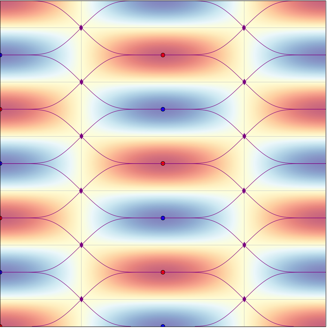
One may get an insight on the counter-example in the proof above by investigating the shape of the Neumann domains obtained from the choice . The eigenfunction (4.7) on the flat torus has Neumann domains of two distinguished shapes, which we call lense-like, and star-like (figure 4.1) . We show in the following that for a sufficiently large value of the eigenfunction restriction to a lense-like Neumann domain does not equal the second eigenvalue of this domain.
Lemma 4.4.
Let be the unit flat 2-dim. torus and its eigenfunction with . Let be a lense-like Neumann domain of . Then such that
Proof.
The major and minor axes of the lense-like Neumann domain, , are of lengths . This Neumann domain is convex and we may apply theorem 1.2(a) of [21]. According to that theorem, for a fixed value of (obeying ) there is a constant ( dependent) such that the nodal set of the second eigenfunction is contained within a vertical strip of width around the center of . Namely, if is the second eigenfunction then , with the origin taken at the center of . Since in our case, the nodal set of is horizontal along (see figure (4.1)), we conclude that for small enough value of the nodal set will not belong to the allowed strip and therefore cannot be the second eigenfunction of . ∎
5. the number of Neumann domains
In this section we denote the number of Neumann domains by
and the number of nodal domains by . If the manifold has boundary,
we denote by the number of
inner and boundary Neumann domains, respectively and have .
For manifolds without boundary we already stated in corollary 1.6,
which we prove below, that the number of Neumann domains is bounded
from below by half the number of nodal domains.
Proof.
[of corollary 1.6] Applying theorem 1.4(vii) with , we have that a Neumann domain contains only a single non self-intersecting nodal line. Hence, each Neumann domain intersects with exactly two nodal domains. It is possible that different Neumann domains intersect with the same nodal domain. The number of nodal domains is therefore bounded from above by . ∎
The same bound holds also for manifolds with boundary. Furthermore,
it may be slightly improved if separating between the count of boundary
and inner Neumann domains.
Corollary 5.1.
[of theorem 3.13]
Let be as in theorem 3.13 and a Morse eigenfunction
on . Then and .
Proof.
[of corollary 5.1] From theorem 3.13(ii) we deduce as in the proof of corollary 1.6 that inner Neumann domains intersect with exactly two nodal domains. From theorem 3.13(v) we deduce that boundary Neumann domains intersect with a single nodal domain. Different Neumann domains may intersect with the same nodal domain and hence . We also get . ∎
The number of Neumann domains may also be studied by examining the graph structure of the Neumann line set. The vertices of such a graph are the critical points and the edges are the Neumann lines connecting them. It is then natural to define the valency of a critical point, , as the number of Neumann lines which are connected to . The following discussion is restricted for the case of manifolds without boundary. Combining Euler’s formula and Morse inequalities we get
| (5.1) |
where are correspondingly the numbers of vertices, edges and faces of the graph. The number of vertices is
| (5.2) |
and the number of edges obeys
| (5.3) |
as at least one endpoint of each edge is a saddle point and all saddles are of valency four. The faces correspond to Neumann domains, , and we therefore get that their number obeys
| (5.4) |
If we further assume a Morse-Smale function we get equalities in both (5.3) and (5.4). We now wish to obtain a lower bound on the number of Neumann domains. Observe that
| (5.5) |
where we used that saddles are of valency four. Plugging (5.2), (5.5) and in (5.1) we get
| (5.6) |
We now assume that the manifold has boundary and is equipped with Dirichlet boundary conditions (as in section 3). We note that each inner Neumann domain has a single minimum and a single maximum on its boundary (theorem 1.4(ii)) and each boundary Neumann domain has either a minimum or a maximum on its boundary (theorem 3.13(iii)). The valency of a critical point equals the number of Neumann domains whose boundary contain this critical point. We therefore obtain for manifolds with boundary
| (5.7) |
which leads to
| (5.8) |
where the right inequality holds as each Neumann line emanating from an extremum ends at a saddle point and each saddle point is connected by Neumann lines to at most four different extremal points. The relations above motivate the study of the extremal points valencies even if just in the distributional sense.
Finally, let us discuss the asymptotics of the Neumann domain count. The existence of subsequences of eigenfunctions whose nodal count goes to infinity was recently proved [16, 22, 23]. In [16] it was done for the arithmetic case and in [22, 23] it was shown for a class of non positively curved manifolds. From corollary 1.6, we conclude that in these cases there exists a subsequence of eigenfunctions whose Neumann domain count goes to infinity as well. Furthermore, numerical experiments suggest that the number of Neumann domains goes to infinity as . This is the case even for sequences of eigenfunctions for which the number of nodal domains is bounded (see for example figure 5.1 which describes the well-known example by Stern given in [13]). However, the statement above does not hold for all metrics. There are known examples of metrics on the torus constructed by Jakobson and Nadirashvili [20], which have subsequences of eigenfunctions corresponding to eigenvalues with uniformly bounded number of critical points. As the saddle points in this example are non-degenerate ones [1], the boundedness of number of saddles implies by (5.4) that the number of Neumann domains for these subsequences is also uniformly bounded. In other words, eigenfunctions corresponding to arbitrarily high eigenvalues might have a small number of Neumann domains.

6. Summary
This paper studies Laplacian eigenfunctions on surfaces by investigating their Neumann domains. Given an eigenfunction, we define Neumann lines and Neumann domains and show that they form a partition of the manifold. Furthermore, we claim that this partition is as natural as the partition dictated by the nodal set. However, numerous essential questions that are being investigated for nodal domains are open for Neumann domains. The current paper develops this study by discussing and answering some of those questions.
Let us specify some points of comparison between Neumann
domains and nodal domains. From a topological point of view, Neumann
domains are simply connected (theorems 1.4(iv)
and 3.13(iv)), whereas nodal
domains are not in general [33, 35]. The
simplicity of the Neumann partition is also apparent in the eigenfunction
restriction to a Neumann domain, . Theorems
1.4 and 3.13 show
that the structure of cannot be too complex
in terms of the position and number of critical points and the nodal
set within . As
is also an eigenfunction of the domain with Neumann boundary
conditions, its structural simplicity suggests that the position of
in the spectrum of cannot be
too high. A similar question for nodal domains is easy to answer and
for each nodal domain of , it is known that
is the first Dirichlet eigenfunction of . This observation was
used by Pleijel [34] to obtain an asymptotic bound on
the nodal domain count. Similarly, answering the analogous question
for Neumann domains would help in estimating the number of Neumann
domains, as is discussed in section 4.2.
In particular, we already show that the number of Neumann domains
is bounded from below by half the number of nodal domains (corollary
1.6) for the types of manifolds
we consider.
It is well known that the number of nodal domains is affected by
the stability of the nodal set. This is apparent for example in the
case of multiple eigenvalues. Such eigenvalues may posses eigenfunctions
where nodal lines intersect. Perturbations of these eigenfunctions
may prevent these crossings and the intersecting lines resolve into
two separate nodal lines. The nature of this resolution of the intersection
crucially affects the topology and number of nodal domains and makes
their counting a difficult task. Neumann domains, however, show a
different behavior. A crossing of nodal lines always occurs at a saddle
point of the function and therefore it also coincides with a Neumann
line intersection. Such a Neumann line crossing is stable with respect
to perturbations and thus there is no change in the number of Neumann
domains when the eigenfunction is perturbed. This was already observed
in [30] and it was suggested that the Neumann line
pattern is relatively robust and hence the relative ease (in comparison
with nodal domains) of the Neumann domain count. Yet, there is an
additional phenomenon which complicates the count of Neumann domains.
Considering a multiple eigenvalue and some non Morse-Smale eigenfunction
which belongs to it, a perturbation might cause an appearance of a
new Neumann domain. Such a domain appears at the Neumann line which
connects some two saddle points and its volume may be arbitrarily
small. The purpose of theorem 4.2
is to place a restriction on the number of such shrinking domains,
by providing a lower bound on the outer radius of some of the Neumann
domains.
Finally, we wish to point out open problems and possible exploration directions for the study of Neumann domains. In the following denotes a two dimensional compact manifold with or without boundary, denotes an eigenpair of the Laplacian on and is some Neumann domain of .
- (i)
Let be a 2-dimensional surface. For a Morse-eigenfunction, , of , denote (see also proposition 1.7 and the preceding discussion)
What conditions on does one need to assure that is either bounded or possesses a bounded subsequence? Such boundedness imposes lower bounds and asymptotic results for the Neumann domain count (see proof of proposition 1.7).
- (ii)
What are the asymptotics of the Neumann domain count? More specifically, does the limit of exist, in general or for some classes of manifolds? If so, could it be bounded from below?
An easier task would be to bound from below. Is it possible to obtain a Courant-like bound? Namely, obtain an upper bound of the form , with being some function (possibly linear). - (iii)
- (iv)
Bounding the total length of the Neumann line set in terms of the eigenvalue.
- (v)
Providing a global upper bound for the volume of a single Neumann domain in terms of the eigenvalue.
- (vi)
Is it possible to improve the lower bound on the outer radius of a Neumann domain in theorem 4.2? The main improvement might be to make this bound global, so that it applies to all Neumann domains of the eigenfunction.
- (vii)
Provide an upper bound on the inner radius of a Neumann domain.
7. Acknowledgments
We are grateful to Thomas Hoffmann-Ostenhof for several enlightening discussions during the course of this work. We thank those who listened to our ideas and helped us to sharpen them: Robert Adler, Gregory Berkolaiko, Michael Berry, Mark Dennis, Stephen Fulling, Dmitry Jakobson, Peter Kuchment, Dan Mangoubi, Uzy Smilansky, Mikhail Sodin and Steve Zelditch. A special thanks goes to Tobias Hartnick for the idea of proof in theorem 1.4(iv) and to Michael Levitin for interesting discussions on the first problem in our list of open questions. Alexander Taylor is warmly acknowledged for providing the code with which the figures were generated. Finally, we thank the referee for the careful reading of the manuscript and their useful suggestions. R.B. was supported by ISF (grant No. 494/14), Marie Curie Actions (grant No. PCIG13-GA-2013-618468) and the Taub Foundations (Taub Fellow). D.F. thanks the mathematics department of the Technion for their hospitality.
References
- [1] Private communication with D. Jakobson.
- [2] A. Banyaga and D. Hurtubise. Lectures on Morse Homology. Kluwer Acad. Pub., 2004.
- [3] G. Blum, S. Gnutzmann, and U. Smilansky. Nodal domains statistics: A criterion for quantum chaos. Physical Review Letters, 88(11):114101, March 2002.
- [4] R. Bott and L. W. Tu. Differential forms in algebraic topology, volume 82 of Graduate Texts in Mathematics. Springer-Verlag, New York-Berlin, 1982.
- [5] J. Bourgain and Z. Rudnick. On the geometry of the nodal lines of eigenfunctions of the two-dimensional torus. Ann. Henri Poincaré, 12(6):1027–1053, 2011.
- [6] J. Bourgain and Z. Rudnick. On the nodal sets of toral eigenfunctions. Invent. Math., 185(1):199–237, 2011.
- [7] J. Brüning. Über Knoten von Eigenfunktionen des Laplace-Beltrami-Operators. Mathematische Zeitschrift, 158(1):15–21, 1978.
- [8] J. Brüning and D. Fajman. On the nodal count for flat tori. Comm. Math. Phys., 313(3):791–813, 2012.
- [9] J. Brüning and D. Gromes. Über die Länge der Knotenlinien schwingender Membranen. Mathematische Zeitschrift, 124(1):79–82, 1972.
- [10] S.Y. Cheng. Eigenfunctions and nodal sets. Comment. Math. Helv., 51(1):43–55, 1976.
- [11] T. H. Colding and W.P. Minicozzi II. Lower bounds for nodal sets of eigenfunctions. Comm. Math. Phys., 306:777, 2011.
- [12] R. Courant. Ein allgemeiner Satz zur Theorie der Eigenfunktione selbstadjungierter Differentialausdrücke. Nachr. Ges. Wiss. Göttingen Math Phys, July K1:81–84, 1923.
- [13] R. Courant and D. Hilbert. Methods of mathematical physics. Vol. I. Interscience Publishers, Inc., New York, N.Y., 1953.
- [14] H. Donnelly and C. Fefferman. Nodal sets of eigenfunctions on Riemannian manifolds. Invent. Math., 93(1):161–183, 1988.
- [15] G. Faber. Beweis, dass unter allen homogenen Membranen von gleicher Fläche und gleicher Spannung die kreisförmige den tiefsten Grundton gibt, Sitzungberichte der mathematisch-physikalischen Klasse der Bayerischen Akademie der Wissenschaften zu München. pages 169–172, 1923.
- [16] A. Ghosh, A. Reznikov, and P. Sarnak. Nodal domains of maass forms i. Geometric and Functional Analysis, 23(5):1515–1568, 2013.
- [17] S. Gnutzmann and U. Smilansky. Complex patterns in wave functions: drums, graphs and disorder. Philosophical Transactions of the Royal Society A, January 2014.
- [18] S. Gnutzmann, U. Smilansky, and N. Sondergaard. Resolving isospectral ’drums’ by counting nodal domains. Journal of Physics A Mathematical General, 38:8921–8933, October 2005.
- [19] H. Hezari and C. D. Sogge. A natural lower bound for the size of nodal sets. Anal. PDE, 5(5):1133–1137, 2012.
- [20] D. Jakobson and N. Nadirashvili. Eigenfunctions with few critical points. J. Differential Geom., 53(1):177–182, 1999.
- [21] D. Jerison. Locating the first nodal line in the neumann problem. Trans. of the Am. Math. So., 352(5):2301–2317, 2000.
- [22] J. Jung and S. Zelditch. Number of nodal domains and singular points of eigenfunctions of negatively curved surfaces with an isometric involution. arXiv:1310.2919 [math.SP], 2013.
- [23] J. Jung and S. Zelditch. Number of nodal domains of eigenfunctions on non-positively curved surfaces with concave boundary. arXiv:1401.4520 [math.SP], 2014.
- [24] D. Klawonn. Inverse nodal problems. J. Phys. A: Math. Theor., 42:175209, August 2009.
- [25] E. Krahn. Über eine von Rayleigh formulierte Minimaleigenschaft des Kreises. Math. Ann., 94(1):97–100, 1925.
- [26] P. Kröger. Upper bounds for the Neumann eigenvalues on a bounded domain in Euclidean space. J. Funct. Anal., 106(2):353–357, 1992.
- [27] D. Mangoubi. Local asymmetry and the inner radius of nodal domains. Comm. Partial Differential Equations, 33:1611–1621, February 2008.
- [28] D. Mangoubi. On the inner radius of a nodal domain. Canad. Math. Bull., 51(2):249–260, 2008.
- [29] D. Mangoubi. The volume of a local nodal domain. J. Topol. Anal., 2(2):259–275, 2010.
- [30] R. B. McDonald and S. A. Fulling. Neumann nodal domains. Phil. Transac. Roy. Soc., A 372:20120505, 2014.
- [31] C. B. Morrey, Jr. and L. Nirenberg. On the analyticity of the solutions of linear elliptic systems of partial differential equations. Comm. Pure Appl. Math., 10:271–290, 1957.
- [32] F. Nazarov, L. Polterovich, and M. Sodin. Sign and area in nodal geometry of laplace eigenfunctions. American Journal of Mathematics, 127(4):pp. 879–910, 2005.
- [33] F. Nazarov and M. Sodin. On the number of nodal domains of random spherical harmonics. Amer. J. Math., 131(5):1337–1357, 2009.
- [34] A. Pleijel. Remarks on courant’s nodal line theorem. Communications on Pure and Applied Mathematics, 9(3):543–550, 1956.
- [35] P. Sarnak and I. Wigman. Topologies of nodal sets of random band limited functions. arXiv:1312.7858.
- [36] M. Schwarz. Morse homology, volume 111 of Progress in Mathematics. Birkhäuser Verlag, Basel, 1993.
- [37] H.-J. Stöckmann and U. Smilansky. Nodal patterns in physics and mathematics. The European Physical Journal Special Topics, June 2007.
- [38] K. Uhlenbeck. Generic properties of eigenfunctions. Amer. J. Math., 98(4):1059–1078, 1976.
- [39] S. Zelditch. Eigenfunctions and nodal sets. Surveys in Differential Geometry, 18:237–308, 2013.
- [40] Afra J. Zomorodian, M. J. Ablowitz, S. H. Davis, E. J. Hinch, A. Iserles, J. Ockendon, and P. J. Olver. Topology for Computing (Cambridge Monographs on Applied and Computational Mathematics). Cambridge University Press, New York, NY, USA, 2005.
Ram Band (corresponding author)
Department of Mathematics, Technion - Israel Institute of
Technology, Haifa 32000, Israel
ramband@technion.ac.il
David Fajman
University of Vienna
David.Fajman@univie.ac.at