Fermi-normal, optical, and wave-synchronous coordinates for spacetime with a plane gravitational wave

Malik Rakhmanov Affiliation: Center for Gravitational Wave Astronomy, Department of Physics, University of Texas at Brownsville, 1 W University Blvd., Brownsville, TX 78520, USA Email: malik.rakhmanov@utb.edu

Abstract

Fermi normal coordinates provide a standardized way to describe the effects of gravitation from the point of view of an inertial observer. These coordinates have always been introduced via perturbation expansions and were usually limited to distances much less than the characteristic length scale set by the curvature of spacetime. For a plane gravitational wave this scale is given by its wavelength which defines the domain of validity for these coordinates known as the long-wavelength regime. The symmetry of this spacetime, however, allows us to extend Fermi normal coordinates far beyond the long-wavelength regime. Here we present an explicit construction for this long-range Fermi normal coordinate system based on the unique solution of the boundary-value problem for spacelike geodesics. The resulting formulae amount to summation of the infinite series for Fermi normal coordinates previously obtained with perturbation expansions. We also consider two closely related normal coordinate systems: optical coordinates which are built from null geodesics and wave-synchronous coordinates which are built from spacelike geodesics locked in phase with the propagating gravitational wave. The wave-synchronous coordinates yield the exact solution of Peres and Ehlers-Kundt which is globally defined. In this case, the limitation of the long-wavelength regime is completely overcome, and the system of wave-synchronous coordinates becomes valid for arbitrarily large distances. Comparison of the different coordinate systems is done by considering the motion of an inertial test mass in the field of a plane gravitational wave.

pacs

04.80.Nn, 07.05.Kf, 95.55.Ym

1 Introduction

In general relativity the choice of coordinates is rather arbitrary and no preference is given to any particular coordinate system ahead of time. However, when the observer wants to describe the effects of gravitation in his vicinity, he may find it convenient to use a quasi-Cartesian coordinate system also known as the local-Lorentz frame. This coordinate system is associated with a reference point in spacetime usually chosen at its origin. A continuous set of quasi-Cartesian (QC) coordinates associated with a reference curve gives rise to what is known as Fermi coordinates [1, 2], if a certain condition is satisfied. Namely, to guarantee uniqueness, one must preclude arbitrary rotations of the QC frame, allowing only the rotation which is caused by the bending of the reference curve. The basis vectors (tetrad) which define the orientation of these coordinates are carried along the curve by means of Fermi-Walker transport. From a mathematical point of view, the Fermi coordinates represent a unique, continuous set of non-rotating QC coordinates, in which the metric is flat and all of its first derivatives vanish on the reference curve, except perhaps the derivative along the curve [1, 2]. From a physical point of view, these are the coordinates that the observer would naturally use to measure distances and times in his vicinity, whereas the reference curve is his worldline in the four-dimensional spacetime [3]. If the observer is freely falling, the reference curve becomes geodesic and the Fermi-Walker transport of the basis vectors becomes parallel transport. In this case, all the first derivatives of the metric vanish on the reference curve and the resulting coordinates are called Fermi normal (FN) [4]. For an accelerating observer the definition of Fermi coordinates is somewhat more complicated but is introduced along the same lines (e.g. [5]). Note that although an observer on Earth is not inertial, one often ignores this fact to simplify calculations. In particular, the effect of gravitational waves on a measuring device (detector) in a laboratory environment on Earth is often described from the point of view of such an inertial observer, neglecting the gravitational field of Earth.

One of the earliest descriptions of a gravitational wave interacting with a detector as viewed by an inertial observer was introduced by Weber [6]. This picture was widely used at the time when resonant bar detectors were operating around the Earth in search of cosmic gravitational waves. It is a curious fact that this approach is largely forgotten today. In modern times of laser-interferometric gravitational wave detectors, the coordinates of choice are those in which a gravitational wave is described by the transverse and traceless tensor and which are often referred to as the TT coordinates or the TT gauge [7]. In these coordinates, one can calculate the response of laser interferometers to gravitational waves with relative ease and with no limit on the distances spanned by these coordinates (e.g. [8]). Similar calculations in FN coordinates are usually more complicated and thus far have always been restricted to distances much less than the wavelength of the gravitational wave, the condition commonly known as the long-wavelength regime. This is mainly why FN coordinates have been gradually displaced by TT coordinates over time.

Historically, the local coordinates associated with an observer have been introduced within different mathematical frameworks and appeared under different names before a standardized approach emerged. In the early days, the coordinate construction would simply be an adaptation of the geodesic deviation equation (e.g. [6, 7]) and, as a result, it was naturally limited to the long-wavelength regime. Pertaining to the center of mass of a resonant bar, such a coordinate system was frequently referred to as the rest frame of the detector. In laser interferometers, a similar coordinate system would be associated with the interferometer beam splitter and therefore would be called the rest frame of the beam splitter. Early analysis of gravitational waves in these coordinates can be found in papers by Grishchuk [9], Grishchuk and Polnaver [10], and Pegoraro et al[11]. In all these cases, the calculations were carried out under the assumption that the distances spanned by these coordinates are much less than the wavelength of the gravitational wave. A more direct approach to the detector coordinates was taken by Fortini and Gualdi [12] who chose the Fermi normal construction as their main tool, cutting short the equation for geodesic deviation. This approach was later adopted by others and gradually became the method of choice when the analysis of gravitational waves had to be carried out from the point of view of an inertial observer [13, 14, 15, 16]. From then on, there was no need to consider closely located geodesics, and yet the distance limitation inherited from the equation for geodesic deviation continued to appear in all subsequent calculations with these coordinates.

More recent interest in the coordinate system of an inertial observer was motivated by the desire to understand better the response of interferometric gravitational-wave detectors. Two different efforts were made to extend the detector response beyond the long-wavelength regime in the local-Lorentz frame [17, 18]. The first targeted linear-frequency corrections to the long-wavelength approximation, whereas the second attempted to obtain formulae to all orders of the perturbation expansion. It was soon realized that the coordinate systems used in these calculations were different even though both approaches were based on the local-Lorentz frame of an inertial observer. The difference in the coordinate systems was the initial motivation for this paper. Another motivation came from the fact that the coordinates utilized in [18] did not have the usual higher-order corrections. By chance, the metric in these coordinates turned out to be equivalent to the exact solution of Peres [19] and Ehlers-Kundt [20], which is globally defined. Different questions naturally appear at this point. What is the relationship between these new coordinates and the Fermi normal frame? And, why is there even an ambiguity in the definition of a normal-coordinate system?

To answer these questions we have to consider the Fermi normal construction in its full generality, i.e. without making approximations with respect to the distances spanned by these coordinates. In this paper, we will show that for a special geometry of spacetime in which a plane gravitational wave is propagating in a flat background, the construction can be carried out to all orders of a perturbation expansion leading to analytical formulae for Fermi normal coordinates which are valid outside the long-wavelength regime. Effectively, this amounts to summation of the infinite series in the perturbation expansion. We will also consider the closely related, optical coordinates that are built upon null geodesics instead of spacelike geodesics of the Fermi scheme. Optical coordinates represent another choice for a normal-coordinate system available to the observer attempting to study the effects of a gravitational wave in his vicinity. Analysis of the boundary-value problem for geodesics defining the normal coordinates shows that there is one more solution. Namely, a special coordinate system can be introduced in which spacelike geodesics extend outward from the observer synchronously with the incoming gravitational wave, and which we will call wave-synchronous coordinates. We will show that these coordinates yield the exact solution of Peres and Ehlers-Kundt, which is why there were no higher-order corrections to the metric associated with these coordinates. This also explains the difference between the coordinate systems in [17] and [18]. The first of these papers involved Fermi normal coordinates whereas the second happened to have the wave-synchronuous system.

The presentation of this paper is organized as follows. Section 1 contains this Introduction. In Section 2 we give a brief overview of Riemann and Fermi normal coordinates. In Section 3 we describe two types of solutions for a geodesic in spacetime with a plane gravitational wave. In Section 4 we introduce an ortho-normal tetrad associated with an inertial observer. In Section 5 we give an explicit construction of Fermi normal coordinates based on the solution of the boundary-value problem for geodesics. In Section 6 we derive the infinite series representation from the exact formulae. In Sections 7 and 8 we give explicit constructions for two other types of normal coordinates: optical and wave-synchronous. In Section 9 we compare the different coordinate systems using the example of an inertial test mass. The Conclusion is given in Section 10. The Appendix contains explicit formulae for the Christoffel coefficients and the Riemann tensor.

2 Overview of Riemann and Fermi normal coordinates

We begin with a brief overview of Riemann and Fermi normal coordinates. Consider an arbitrary spacetime with coordinates $x^{\mu}$ , where $\mu=0,1,2,3$ , implying as usual that the first of these coordinates is timelike and the rest are spacelike. Let the associated metric be $g_{\mu\nu}$ . At any given point, $P_{0}=\{x_{0}^{\mu}\}$ , the metric tensor can be diagonalized by an orthogonal transformation and the resulting diagonal elements can then be scaled to $\pm 1$ , rendering the metric in the Minkowski form:

\bar{g}_{\mu\nu}(x_{0})=\eta_{\mu\nu},

(1)

where $\eta_{\mu\nu}=\mathrm{diag}\{-1,1,1,1\}$ . In the vicinity of this reference point, a coordinate system $\bar{x}^{\mu}$ can be introduced in such a way that the metric remains as close to the Minkowski form as possible in curved spacetime. In particular, one can make sure that there are no first-order corrections to the metric by enforcing the condition:

\bar{g}_{\mu\nu,\alpha}(x_{0})=0,

(2)

where comma stands for differentiation with respect to the new coordinates. This condition is usually achieved by making the coordinate lines for the new coordinate system as close to straight lines as they can possibly be in curved spacetime, i.e. along geodesics. Note that one cannot impose a similar condition on the second derivatives of the metric unless the curvature of spacetime vanishes at this point. The resulting coordinates $\bar{x}^{\mu}$ are known as Riemann normal coordinates. They are the closest thing to a Cartesian frame that an observer can build in curved spacetime in the vicinity of one point and one instance of time. In general, the metric contains nonzero second derivatives and its expansion near the reference point takes the form:

\bar{g}_{\mu\nu}=\eta_{\mu\nu}-\frac{1}{3}\hat{R}_{\mu\rho\nu\sigma}\,\bar{x}^{\rho}\bar{x}^{\sigma}+\ldots,

(3)

where the dots stand for higher-order terms. In what follows the hat above some function will always mean that the value of this function is taken at the reference point, e.g.,

\hat{R}_{\mu\rho\nu\sigma}\equiv R_{\mu\rho\nu\sigma}(x_{0}).

(4)

The Riemann normal coordinates are tied to the reference point which serves as the origin for this coordinate system. Take another point, and the whole construction must be repeated yielding a coordinate system which may not be connected with the first one in any obvious way. This observation prompted Fermi [1] to introduce a different coordinate system – one which is built around a reference curve rather than a point. In Fermi’s construction, one starts with an arbitrary timelike curve and chooses the parameter along the curve as the first new coordinate $\bar{x}^{0}$ . The remaining coordinates $\bar{x}^{i}$ , for $i=1,2,3$ are built via geodesics which are orthogonal to the reference curve and to each other. This approach guarantees that the derivatives of the metric with respect to these remaining coordinates vanish when evaluated on the reference curve. The derivative with respect to the first coordinate may not be zero. If the reference curve itself is geodesic, then all the first derivatives of the metric vanish and the resulting coordinates are called Fermi normal. They are the closest thing to a Cartesian frame that an inertial observer can build in curved spacetime in the vicinity of his worldline. The expansion of the metric near the reference curve takes the form:

$\displaystyle\bar{g}_{00}$	$\displaystyle=$	$\displaystyle-1-\hat{R}_{0k0l}\,\bar{x}^{k}\bar{x}^{l}+\ldots,$	(5)
$\displaystyle\bar{g}_{0j}$	$\displaystyle=$	$\displaystyle-\frac{2}{3}\hat{R}_{0kjl}\,\bar{x}^{k}\bar{x}^{l}+\ldots,$	(6)
$\displaystyle\bar{g}_{ij}$	$\displaystyle=$	$\displaystyle\delta_{ij}-\frac{1}{3}\hat{R}_{ikjl}\,\bar{x}^{k}\bar{x}^{l}+\ldots,$	(7)

which no longer has the symmetry between the timelike and spacelike coordinates present in the Riemann form (3). Equations (5)–(7) represent the metric in Fermi normal coordinates to second order in the perturbation expansion with respect to distance parameters. They were first derived¹¹ 1 The definition for the Riemann tensor adopted in [4] differs from ours by an overall sign. by Manasse and Misner [4]. Significant effort is needed to go beyond the second-order approximation and generally such calculations can be very complicated. The third- and fourth-order approximations for Fermi normal coordinates in arbitrary spacetime were derived by Li and Ni [21, 22].

The next important result was obtained by Fortini and Gualdi [12] who succeeded in deriving the series expansion to all orders in the distance parameters for spacetime in which a plane gravitational wave is propagating in a flat background. The formulae of Fortini and Gualdi were later generalized by Marzlin [23] for an arbitrary weak-field geometry of spacetime and accelerating observers. Marzlin’s formulae for the metric in the case of a non-accelerating observer are

$\displaystyle\bar{g}_{00}$	$\displaystyle=$	$\displaystyle-1-2\sum_{n=0}^{\infty}\frac{n+3}{(n+3)!}\hat{R}_{0k0l,m_{1}\ldots m_{n}}\,\bar{x}^{k}\bar{x}^{l}\bar{x}^{m_{1}}\ldots\bar{x}^{m_{n}},$	(8)
$\displaystyle\bar{g}_{0j}$	$\displaystyle=$	$\displaystyle-2\sum_{n=0}^{\infty}\frac{n+2}{(n+3)!}\hat{R}_{0kjl,m_{1}\ldots m_{n}}\,\bar{x}^{k}\bar{x}^{l}\bar{x}^{m_{1}}\ldots\bar{x}^{m_{n}},$	(9)
$\displaystyle\bar{g}_{ij}$	$\displaystyle=$	$\displaystyle\delta_{ij}-2\sum_{n=0}^{\infty}\frac{n+1}{(n+3)!}\hat{R}_{ikjl,m_{1}\ldots m_{n}}\,\bar{x}^{k}\bar{x}^{l}\bar{x}^{m_{1}}\ldots\bar{x}^{m_{n}},$	(10)

where comma preceding indices $m_{1}\ldots m_{n}$ denotes differentiation with respect to these coordinates, e.g.,

\hat{R}_{\mu k\nu l,m_{1}\ldots m_{n}}\equiv\left.\frac{\partial^{n}R_{\mu k\nu l}}{\partial x^{m_{1}}\ldots\partial x^{m_{n}}}\right|_{x=x_{0}}.

(11)

The infinite series, (8)–(10), include the second-order metric of Manasse and Misner, and the third- and fourth-order metrics of Li and Ni as special cases.

3 Spacetime with a plane gravitational wave

3.1 Metric tensor and fundamental form

Within the linearized approach, a gravitational wave propagating in empty space is described by a small perturbation $h_{\mu\nu}$ to the otherwise flat metric:

g_{\mu\nu}=\eta_{\mu\nu}+h_{\mu\nu}.

(12)

The corresponding fundamental form is defined as

F=g_{\mu\nu}\,\rmd x^{\mu}\,\rmd x^{\nu},

(13)

in some coordinate system $x^{\mu}$ . Assume that in the absence of the gravitational wave, i.e. when $h_{\mu\nu}=0$ , three of these coordinates become the usual Cartesian coordinates,

x^{1}\equiv x,\quad x^{2}\equiv y,\quad x^{3}\equiv z.

(14)

and the remaining coordinate becomes time

x^{0}\equiv\tau=ct,

(15)

where $c$ is the speed of light in flat spacetime. We will use this naming convention even for curved spacetime, i.e. when $h_{\mu\nu}\neq 0$ , keeping in mind that the meaning of these coordinates is fundamentally different from that of the Newtonian world and that the small correction to the metric (12) changes their interpretation (see Section 9).

A number of components of the symmetric tensor $h_{\mu\nu}$ can be set to zero by choosing the transverse and traceless gauge [7]. The remaining components,

	$\displaystyle h_{xx}=-h_{yy}$	$\displaystyle\equiv$	$\displaystyle h_{+}(\tau+z),$		(16)
	$\displaystyle h_{xy}=h_{yx}$	$\displaystyle\equiv$	$\displaystyle h_{\times}(\tau+z),$		(17)

represent two independent degrees of freedom of the gravitational wave, commonly known as the $+$ and $\times$ polarizations. The gauge fixes the orientation of the coordinate system in such a way that the gravitational wave is propagating in the negative- $z$ direction and its transverse polarizations belong to the $xy$ plane. In these coordinates, the fundamental form is given by

	$\displaystyle F$	$\displaystyle=$	$\displaystyle-\rmd\tau^{2}+\rmd x^{2}+\rmd y^{2}+\rmd z^{2}+$		(18)
			$\displaystyle h_{+}(\tau+z)\;(\rmd x^{2}-\rmd y^{2})+2h_{\times}(\tau+z)\;\rmd x\,\rmd y.$		(18)

One can also introduce a natural measure, $\sigma$ , such that

F=\epsilon\,\rmd\sigma^{2}.

(19)

To ensure that $\rmd\sigma$ is real we choose $\epsilon=1$ or $-1$ depending on whether the fundamental form is positive or negative definite.

We also introduce two auxiliary coordinates,

u=\tau+z\qquad{\mathrm{and}}\qquad v=\tau-z,

(20)

which sometimes will be more convenient than $\tau$ and $z$ . For example, the propagation of the plane front of the gravitational wave is described by $u=\mathrm{const}$ . In terms of $u$ and $v$ , the fundamental form (18) is given by

F=-\rmd u\,\rmd v+\rmd x^{2}+\rmd y^{2}+h_{+}(u)(\rmd x^{2}-\rmd y^{2})+2h_{\times}(u)\,\rmd x\,\rmd y.

(21)

We do not assume any particular form for the functions

h_{a}=h_{a}(u),\qquad{\mathrm{where}}\qquad a=+,\times.

(22)

They can be completely arbitrary as long as they represent some physically possible waveforms.

Within the linearized theory of gravitation we only need to keep track of terms which are first order in $h_{a}$ . Second and higher order terms are neglected. Hence, we will be freely replacing any expression containing $h_{a}$ with its linear (first-order in $h_{a}$ ) approximation throughout this paper.

3.2 Geodesic equation

The construction of normal coordinates relies on the explicit solution of the geodesic equation. Here we describe the solution for geodesics following closely the derivation in [24]. Let $x^{\mu}(\sigma)$ be a continuous curve in this spacetime and $p^{\mu}(\sigma)$ be a tangent vector for this curve:

p^{\mu}=\frac{\rmd x^{\mu}}{\rmd\sigma}\qquad{\mathrm{and}}\qquad p_{\mu}=g_{\mu\nu}\,p^{\nu}.

(23)

Explicit formulae for the covariant components of the tangent vector are

$\displaystyle p_{v}$	$\displaystyle=$	$\displaystyle-\frac{1}{2}\frac{\rmd u}{\rmd\sigma},$	(24)
$\displaystyle p_{x}$	$\displaystyle=$	$\displaystyle\left[1+h_{+}(u)\right]\frac{\rmd x}{\rmd\sigma}+h_{\times}(u)\frac{\rmd y}{\rmd\sigma},$	(25)
$\displaystyle p_{y}$	$\displaystyle=$	$\displaystyle\left[1-h_{+}(u)\right]\frac{\rmd y}{\rmd\sigma}+h_{\times}(u)\frac{\rmd x}{\rmd\sigma},$	(26)
$\displaystyle p_{u}$	$\displaystyle=$	$\displaystyle-\frac{1}{2}\frac{\rmd v}{\rmd\sigma}.$	(27)

Assume that $\sigma$ is the natural measure along the curve. Then by virtue of (19) the tangent vector becomes normalized,

p_{\mu}p^{\mu}=\epsilon,

(28)

where now the indicator $\epsilon$ takes values $-1,1$ , or $0$ , depending on whether the tangent vector is timelike, spacelike, or null. The normalization condition, written in terms of the covariant components, is given by

-4p_{u}p_{v}+p_{x}^{2}[1-h_{+}(u)]+p_{y}^{2}[1+h_{+}(u)]-2p_{x}p_{y}\,h_{\times}(u)=\epsilon.

(29)

Next, assume that the curve $x^{\mu}(\sigma)$ is a geodesic. Then the tangent vector satisfies the equation

\frac{\rmd p_{\alpha}}{\rmd\sigma}=\frac{1}{2}h_{\mu\nu,\alpha}\,p^{\mu}p^{\nu}.

(30)

Or, equivalently,

\frac{\rmd p_{u}}{\rmd\sigma}=\frac{1}{2}\left(p_{x}^{2}-p_{y}^{2}\right)h^{\prime}_{+}(u)+p_{x}p_{y}h^{\prime}_{\times}(u),

(31)

and

\frac{\rmd p_{v}}{\rmd\sigma}=0,\qquad\frac{\rmd p_{x}}{\rmd\sigma}=0,\qquad\frac{\rmd p_{y}}{\rmd\sigma}=0.

(32)

Therefore, three components of the tangent vector are constant along the geodesic:

$\displaystyle p_{v}$	$\displaystyle=$	$\displaystyle p_{v0},$	(33)
$\displaystyle p_{x}$	$\displaystyle=$	$\displaystyle p_{x0},$	(34)
$\displaystyle p_{y}$	$\displaystyle=$	$\displaystyle p_{y0}.$	(35)

The fourth component, $p_{u}$ , can be found from the normalization condition (29):

p_{u}=\frac{1}{4p_{v0}}\left[-\epsilon+p_{x0}^{2}+p_{y0}^{2}-(p_{x0}^{2}-p_{y0}^{2})\,h_{+}(u)-2p_{x0}p_{y0}\,h_{\times}(u)\right],

(36)

where for the moment we assumed that $p_{v0}\neq 0$ . It turns out that this is not always the case. The solutions for the geodesic equation which correspond to $p_{v0}\neq 0$ will be called main or non-singular and the solutions which correspond $p_{v0}=0$ will be called singular. Note that the main or non-singular solution allows all three types of geodesics: timelike, spacelike, and null, whereas the singular solution allows only spacelike geodesics. The calculations proceed differently for the singular and non-singular cases.

3.3 The non-singular solution of the geodesic equation

The main or non-singular solution of the geodesic equation takes place if

p_{v0}\neq 0.

(37)

In this case, integration of equation (24) yields the solution for $u$ :

u(\sigma)=u_{0}-2p_{v0}\sigma,

(38)

where $u_{0}$ is the initial value for this coordinate. This solution alone completely defines the gravitational wave amplitudes on the geodesic:

h_{a}=h_{a}[u(\sigma)].

(39)

Next, inverting (25) and (26) to first order in $h$ , we obtain

	$\displaystyle\frac{\rmd x}{\rmd\sigma}$	$\displaystyle=$	$\displaystyle p_{x0}\,\left\{1-h_{+}[u(\sigma)]\right\}-p_{y0}\,h_{\times}[u(\sigma)],$		(40)
	$\displaystyle\frac{\rmd y}{\rmd\sigma}$	$\displaystyle=$	$\displaystyle p_{y0}\,\left\{1+h_{+}[u(\sigma)]\right\}-p_{x0}\,h_{\times}[u(\sigma)].$		(41)

Integration of these equations yields the solution for $x$ and $y$ :

	$\displaystyle x(\sigma)$	$\displaystyle=$	$\displaystyle x_{0}+p_{x0}\sigma\left[1-f_{+}(\sigma)\right]-p_{y0}\sigma f_{\times}(\sigma),$		(42)
	$\displaystyle y(\sigma)$	$\displaystyle=$	$\displaystyle y_{0}+p_{y0}\sigma\left[1+f_{+}(\sigma)\right]-p_{x0}\sigma f_{\times}(\sigma),$		(43)

where $x_{0}$ and $y_{0}$ are the initial values for these coordinates. In the last two equations we introduced the average polarization amplitudes of the gravitational wave,

f_{a}(\sigma)=\frac{1}{\sigma}\int_{0}^{\sigma}h_{a}[u(\sigma^{\prime})]\,\rmd\sigma^{\prime}.

(44)

Note that $|f_{a}|\leq\max|h_{a}|$ and therefore, $f_{a}$ is at most the same order of magnitude as $h_{a}$ .

Consider now equation (36). Since $h_{a}$ are now fully defined along the geodesic (39), this equation yields $p_{u}$ as a function of $\sigma$ :

	$\displaystyle p_{u}(\sigma)$	$\displaystyle=$	$\displaystyle\frac{1}{4p_{v0}}\left\{-\epsilon+p_{x0}^{2}+p_{y0}^{2}-\right.$		(45)
			$\displaystyle\left.(p_{x0}^{2}-p_{y0}^{2})\,h_{+}[u(\sigma)]-2p_{x0}p_{y0}\,h_{\times}[u(\sigma)]\right\}.$		(45)

Then the solution for $v$ can be obtained from (27):

v(\sigma)=v_{0}-2\int_{0}^{\sigma}p_{u}(\sigma^{\prime})\,\rmd\sigma^{\prime},

(46)

where $v_{0}$ is the initial value for this coordinate. We will also need the solution for $z$ and $\tau$ :

	$\displaystyle z(\sigma)$	$\displaystyle=$	$\displaystyle z_{0}-p_{v0}\sigma+\int_{0}^{\sigma}p_{u}(\sigma^{\prime})\,\rmd\sigma^{\prime},$		(47)
	$\displaystyle\tau(\sigma)$	$\displaystyle=$	$\displaystyle\tau_{0}-p_{v0}\sigma-\int_{0}^{\sigma}p_{u}(\sigma^{\prime})\,\rmd\sigma^{\prime}.$		(48)

where $z_{0}$ and $\tau_{0}$ are the initial values for these coordinates ( $u_{0}=\tau_{0}+z_{0}$ and $v_{0}=\tau_{0}-z_{0}$ ). This concludes the solution for the geodesic equation in the non-singular case.

The average amplitudes $f_{a}$ will play an important role in all the following calculations. Changing variables in (44), we obtain an alternative definition for $f_{a}$ :

f_{a}(u_{0},u)=\frac{1}{u-u_{0}}\int_{u_{0}}^{u}h_{a}(u^{\prime})\,\rmd u^{\prime},

(49)

which will sometimes be more convenient than (44).

3.4 The singular solution of the geodesic equation

The singular solution of the geodesic equation takes place if

p_{v0}=0.

(50)

This condition together with (24) implies that $u$ is constant along the geodesic:

u(\sigma)=u_{0}.

(51)

Since $u$ is constant, the amplitudes of the gravitational wave are also constant along the geodesic:

h_{a}(u)=h_{a}(u_{0}),

(52)

and therefore,

f_{a}(\sigma)=h_{a}(u_{0}).

(53)

Then the solution for $x$ and $y$ can be obtained by integrating (40) and (41):

	$\displaystyle x(\sigma)$	$\displaystyle=$	$\displaystyle x_{0}+p_{x0}\,\sigma\,[1-h_{+}(u_{0})]-p_{y0}\,\sigma\,h_{\times}(u_{0}),$		(54)
	$\displaystyle y(\sigma)$	$\displaystyle=$	$\displaystyle y_{0}+p_{y0}\,\sigma\,[1+h_{+}(u_{0})]-p_{x0}\,\sigma\,h_{\times}(u_{0}).$		(55)

Note that we can no longer use the normalization condition (29) to find $p_{u}$ . Instead, we shall find $p_{u}$ by solving (31). Not only $h_{a}(u)$ are constant along the geodesic but also $h_{a}^{\prime}(u)$ are constant. Consequently, the entire right-hand side of (31) is constant along the geodesic. Denote this constant by $2A$ :

2A\equiv\frac{1}{2}\left(p_{x0}^{2}-p_{y0}^{2}\right)h^{\prime}_{+}(u_{0})+p_{x0}p_{y0}\,h^{\prime}_{\times}(u_{0}).

(56)

Then equation (31) becomes

\frac{\rmd p_{u}}{\rmd\sigma}=2A.

(57)

Its integration yields

p_{u}(\sigma)=2A\,\sigma+B,

(58)

where $B$ is an arbitrary constant. Finally, integrating (27), we obtain

v(\sigma)=v_{0}-2A\sigma^{2}-2B\sigma,

(59)

where $v_{0}$ is the initial value for this coordinate. We will also need the solution for $z$ and $\tau$ :

	$\displaystyle z(\sigma)$	$\displaystyle=$	$\displaystyle z_{0}+A\sigma^{2}+B\sigma,$		(60)
	$\displaystyle\tau(\sigma)$	$\displaystyle=$	$\displaystyle\tau_{0}-A\sigma^{2}-B\sigma,$		(61)

4 Inertial observer and the orthonormal tetrad

4.1 The observer’s worldline

One consequence of the solution for the geodesic equation is of particular interest. This is the notion that an inertial mass which is initially at rest in the field of a plane gravitational wave remains at rest indefinitely [7, 9]. Also, an inertial mass which is moving along the direction of the gravitational wave propagation ( $\pm z$ ) remains unaffected by the gravitational wave. This can be easily seen from the main solution for geodesics given by (42), (43), (47), and (48), in which we set $\epsilon=-1$ and replace $\sigma$ with $s$ . Note that in this case, the geodesic is timelike and the affine parameter $s$ stands for the proper time. Assume that at the beginning of the geodesic $\rmd x/\rmd s=0$ and $\rmd y/\rmd s=0$ , which means that $p_{x0}=p_{y0}=0$ . Therefore, equations (42) and (43), become

x(s)=x_{0}\qquad{\mathrm{and}}\qquad y(s)=y_{0}.

(62)

Next, equations (47) and (48) can be written as

	$\displaystyle z(s)$	$\displaystyle=$	$\displaystyle z_{0}+p^{z}\,s,$		(63)
	$\displaystyle\tau(s)$	$\displaystyle=$	$\displaystyle\tau_{0}+p^{\tau}\,s,$		(64)

where the constant $p^{z}$ is defined by $\rmd z/\rmd s$ at the initial point on the geodesic, and $p^{\tau}=\sqrt{1+(p^{z})^{2}}$ . Thus, the mass which was initially moving along the $z$ direction continues its motion seemingly un-affected by the gravitational wave.

Since the metric in (18) is invariant under Lorentz transformations in the $z\tau$ plane, we can always transfer to the co-moving coordinate system to achieve $p^{z}=0$ . Then, in addition to (62), we will have

z(s)=z_{0}.

(65)

In these coordinates $p^{\tau}=1$ . Consequently,

\tau(s)=s,

(66)

where we set to zero the arbitrary constant of integration $\tau_{0}$ introduced in equation (64). Therefore, the proper time of the mass, $s$ , coincides with the coordinate time, $\tau$ , for an arbitrary gravitational wave $h_{a}(u)$ .

All these arguments can also be applied to an observer who is moving freely in the field of a gravitational wave, i.e. an inertial observer. Namely, the formulae in this Section can be used to describe the observer’s worldline, which is a timelike geodesic with affine parameter $s$ measuring the observer’s proper time. It follows then that an observer who is initially at rest in the field of a gravitational wave remains at rest indefinitely. In this regard, he appears to be un-affected by the gravitational wave. The observer’s clock, which was initially synchronized with the coordinate time, continues reading the coordinate time even in the presence of the gravitational wave. Also, the clock appears to be un-affected by the gravitational wave. These notions turn out to be artifacts of the present coordinate system (TT gauge). In normal coordinates, an inertial mass will be moving in response to gravitational waves (see Section 9) and the clock will not stay synchronized with the coordinate time.

4.2 Orthonormal tetrad

To define a quasi-Cartesian coordinate system in his vicinity, an observer first needs to introduce four basis vectors, a tetrad, which we denote here as $\lambda^{\bar{\alpha}}$ , where $\bar{\alpha}=0,1,2,3$ . The components of the basis vectors are $(\lambda^{\bar{\alpha}})_{\mu}\equiv\lambda^{\bar{\alpha}}{}_{\mu}$ . Here the index with overline denotes the vector’s order number whereas the index without overline denotes the vector’s component, which in this case is covariant. The contravariant components are defined according to the usual rule:

\lambda^{\bar{\alpha}\mu}=g^{\mu\nu}\,\lambda^{\bar{\alpha}}{}_{\nu}.

(67)

By definition, the basis vectors are ortho-normal:

\lambda^{\bar{\alpha}}{}_{\mu}\,\lambda^{\bar{\beta}}{}^{\mu}=\eta^{\bar{\alpha}\bar{\beta}}.

(68)

Since the observer needs to carry the tetrad with him to the future, the basis vectors must be transported along the observer’s worldline, which is the reference curve. The result is a one-parameter family: $\lambda^{\bar{\alpha}}{}_{\mu}(s)$ , where $s$ is the measure along the reference curve. For a tetrad to be non-rotating, it must be carried along the curve by means of Fermi-Walker transport [4]. If the observer is freely falling, the Fermi-Walker transport becomes parallel transport:

\frac{\rmd\lambda^{\bar{\alpha}}{}_{\nu}}{\rmd s}=\Gamma^{\mu}{}_{\beta\nu}\,p^{\beta}\lambda^{\bar{\alpha}}{}_{\mu},

(69)

where $\Gamma^{\mu}{}_{\beta\nu}$ are the Christoffel coefficients (A). Note that these equations are satisfied independently by each vector $\mathbf{\lambda}^{\bar{\alpha}}$ .

As we have seen, an observer at rest remains at rest indefinitely. In this case, $p^{\mu}=\{1,0,0,0\}$ and equation (69) becomes

\frac{\rmd\lambda^{\bar{\alpha}}{}_{\nu}}{\rmd s}=\Gamma^{\mu}{}_{0\nu}\,\lambda^{\bar{\alpha}}{}_{\mu}.

(70)

This equation has infinite number of solutions all of which correspond to tetrads connected to each other by arbitrary rotations, and which, therefore, are all equivalent. To remove this degeneracy, we assume that in the absence of the gravitational wave, the tetrad is consonant with the coordinate system, i.e. $\lambda^{\bar{\alpha}}{}_{\mu}=\delta^{\bar{\alpha}}{}_{\mu}$ if $h_{a}=0$ . Then the solution of (69) becomes unique and to first order in $h$ is given by

\lambda^{\bar{\alpha}}{}_{\mu}(s)=\delta^{\bar{\alpha}}{}_{\mu}+\frac{1}{2}h^{\bar{\alpha}}{}_{\mu}(s),

(71)

or, equivalently,

\lambda^{\bar{\alpha}{\mu}}(s)=\eta^{\bar{\alpha}{\mu}}-\frac{1}{2}h^{\bar{\alpha}{\mu}}(s).

(72)

Parallel transport of the basis vectors along the geodesic can now be achieved simply by advancing parameter $s$ in the right-hand side of (71) and (72).

Naturally, the use of this tetrad is limited to freely falling observers. To consider an observer on Earth one has to include the observer’s acceleration due to the normal forces which compensate the gravitational pull of the planet or the acceleration due to rotations of the laboratory frame (e.g. [5, 22, 23]).

5 Fermi normal coordinates

We now proceed to the construction of Fermi normal coordinates associated with the worldline of an inertial observer. While the principal directions for the new coordinate system are set by the tetrad, the values for these coordinates are defined by the distances along the geodesics which originate from the location of the observer and reach every point in the observer’s vicinity. Thus, we need to solve a boundary-value problem: for every point in this spacetime we need to find a geodesic which connects it with the observer at a certain point on his worldline. The choice of this point is not unique and will lead to different constructions of the quasi-Cartesian frames. Only one of them corresponds to Fermi normal frame. The geodesic which connects the observer with the particular point in spacetime will be called the connecting geodesic so as to distinguish it from the reference geodesic, which is the worldline of the observer. (The affine parameter on the connecting geodesic will be denoted by $\sigma$ , whereas the parameter on the reference geodesic will remain $s$ .)

5.1 Boundary-value problem for the connecting geodesics

Take an arbitrary point in spacetime $P_{1}=\{x^{\mu}\}$ and connect it with the worldline of the observer via a spacelike geodesic, $x^{\mu}=x^{\mu}(\sigma)$ , where the affine parameter $\sigma$ takes values from interval $[0,\sigma_{1}]$ . Let the tangent vector along the geodesic be $p^{\mu}=\rmd x^{\mu}/\rmd\sigma$ . This connecting geodesic will intersect the observer’s worldline at a some point $P_{0}=\{x_{0}^{\mu}\}$ . Following Fermi, we require that the connecting geodesic cut the observer’s worldline orthogonally, i.e.

\left.p^{\tau}\right|_{\sigma=0}=0.

(73)

Physically, this condition implies that the connecting geodesic is the closest thing to the instantaneous line in this spacetime, as illustrated in figure 1. Mathematically, equation (73) defines the location of point $P_{0}$ on the observer’s worldline.

Refer to caption — Figure 1: The observer’s worldline $z=0$ and the connecting geodesic $P_{0}P_{1}$ in the boundary-value problem for Fermi normal coordinates. Negative values of parameter $\sigma$ correspond to the extension of the connecting geodesic into the past. The inverse of $P_{1}=\{\tau,x,y,z\}$ is $P_{2}\approx\{2s-\tau,-x,-y,-z\}$ .

In what follows, it will be convenient to think of $P_{0}$ as the starting point on the connecting geodesic ( $\sigma=0$ ) and $P_{1}$ as the end point ( $\sigma=\sigma_{1}$ ). Consider the main (non-singular) solution for a geodesic from Section 3.3 and apply it to the connecting geodesic $P_{0}P_{1}$ . Note that we cannot take the singular solution because the constraint (50) is incompatible with the condition for orthogonality (73).

To simplify the following calculations we make a few notational changes. Assume that the observer is located at the spatial origin of the coordinate system:

x_{0}=y_{0}=z_{0}=0.

(74)

Since the coordinate time at point $P_{0}$ coincides with the proper time of the observer (66), we have

\tau_{0}=s,\qquad{\mathrm{and}}\qquad u_{0}=v_{0}=s.

(75)

In this notation, the connecting geodesic starts at $P_{0}=\{s,0,0,0\}$ and ends at $P_{1}=\{\tau,x,y,z\}$ . Alternatively, we can use the $u,v$ coordinates instead of $\tau,z$ and denote the end point as $P_{1}=\{u,x,y,v\}$ . Then the starting point will be $P_{0}=\{s,0,0,s\}$ . Also we introduce compact notation for $h_{a}$ at $P_{1}$ and $P_{0}$ :

	$\displaystyle h_{a}$	$\displaystyle\equiv$	$\displaystyle\left.h_{a}\right\|_{P_{1}}=h_{a}(u),$		(76)
	$\displaystyle\hat{h}_{a}$	$\displaystyle\equiv$	$\displaystyle\left.h_{a}\right\|_{P_{0}}=h_{a}(s).$		(77)

The solution for the geodesic equation (Section 3.3) connects the coordinates of points $P_{0}$ and $P_{1}$ :

$\displaystyle u$	$\displaystyle=$	$\displaystyle s-2p_{v0}\sigma_{1},$	(78)
$\displaystyle x$	$\displaystyle=$	$\displaystyle p_{x0}\,\sigma_{1}\,(1-f_{+})-p_{y0}\,\sigma_{1}\,f_{\times},$	(79)
$\displaystyle y$	$\displaystyle=$	$\displaystyle p_{y0}\,\sigma_{1}\,(1+f_{+})-p_{x0}\,\sigma_{1}\,f_{\times},$	(80)
$\displaystyle v$	$\displaystyle=$	$\displaystyle s-\frac{\sigma_{1}}{2p_{v0}}\left[-\epsilon+p_{x0}^{2}+p_{y0}^{2}-(p_{x0}^{2}-p_{y0}^{2})f_{+}-2\,p_{x0}p_{y0}f_{\times}\right],$	(81)

where $\epsilon=1$ and $f_{a}$ is given by

f_{a}=\frac{1}{u-s}\int_{s}^{u}h_{a}(u^{\prime})\,\rmd u^{\prime}.

(82)

The boundary-value problem is to determine arbitrary constants $p_{v0}$ , $p_{x0}$ , $p_{y0}$ , $s$ , $\sigma_{1}$ in terms of the coordinates of point $P_{1}$ .

Due to nonlinear nature of the boundary-value problem the solution consists of several steps. First, we find the components of the tangent vector from (78)–(80):

$\displaystyle p_{v0}$	$\displaystyle=$	$\displaystyle-\frac{1}{2\sigma_{1}}(u-s),$	(83)
$\displaystyle p_{x0}$	$\displaystyle=$	$\displaystyle(1+f_{+})\frac{x}{\sigma_{1}}+f_{\times}\,\frac{y}{\sigma_{1}},$	(84)
$\displaystyle p_{y0}$	$\displaystyle=$	$\displaystyle(1-f_{+})\frac{y}{\sigma_{1}}+f_{\times}\,\frac{x}{\sigma_{1}}.$	(85)

We shall not be concerned with the fact that $s$ and $\sigma_{1}$ are unknown at this point. We will have to come back to these equations after we determine $s$ and $\sigma_{1}$ . Substituting (83)–(85) into (81), we obtain

(u-s)(v-s)=-\sigma_{1}^{2}+x^{2}+y^{2}+(x^{2}-y^{2})\,f_{+}+2xy\,f_{\times}.

(86)

The next step involves the orthogonality condition (73). Since $p^{\tau}=-p_{v0}-p_{u}$ we can express this condition as

\left.p_{u}\right|_{\sigma=0}=-p_{v0}.

(87)

With the explicit form for $p_{u}$ , equation (45), this condition becomes

4p_{v0}^{2}=1-p_{x0}^{2}-p_{y0}^{2}+(p_{x0}^{2}-p_{y0}^{2})\hat{h}_{+}+2p_{x0}p_{y0}\hat{h}_{\times}.

(88)

Substituting (83)–(85) in (88), we obtain

(u-s)^{2}=\sigma_{1}^{2}-x^{2}-y^{2}-(x^{2}-y^{2})(2f_{+}-\hat{h}_{+})-2xy(2f_{\times}-\hat{h}_{\times}).

(89)

The nonlinear equations (86) and (89) are the key formulae in the boundary-value problem.

We can now find the solution for $s$ . Combining (89) with (86), we eliminate $\sigma_{1}^{2}$ with the result

2(s-\tau)(u-s)=(x^{2}-y^{2})(f_{+}-\hat{h}_{+})+2xy(f_{\times}-\hat{h}_{\times}).

(90)

This equation can be written in the following equivalent form:

s=\tau+\frac{1}{2(u-s)}\left[(x^{2}-y^{2})(f_{+}-\hat{h}_{+})+2xy(f_{\times}-\hat{h}_{\times})\right].

(91)

It defines $s$ as an implicit function of the coordinates of the end point. One can use this equation as an iteration formula to determine $s$ because the terms in the square brackets are of order $h$ . We should not be concerned with the apparent singularity of this formula as $u\rightarrow s$ . One can easily prove that

\frac{f_{a}-\hat{h}_{a}}{u-s}\rightarrow\frac{1}{2}h_{a}^{\prime}(s)

(92)

in this limit.

For completeness, we obtain an explicit formula for $s$ to first order in $h$ . The orthogonality condition (73) implies that in the absence of the gravitational wave $s=\tau$ . Then $u-s\approx z$ to first order in $h$ . We can substitute this approximation in (91) and obtain

s\approx\tau+\frac{1}{2z}\left[(x^{2}-y^{2})(f_{+}-\hat{h}_{+})+2xy(f_{\times}-\hat{h}_{\times})\right].

(93)

Moreover, to first order in $h$ we can replace every occurrance of $s$ with $\tau$ in the right-hand side of this equation. Then

	$\displaystyle\hat{h}_{a}$	$\displaystyle\approx$	$\displaystyle h_{a}(\tau),$		(94)
	$\displaystyle f_{a}$	$\displaystyle\approx$	$\displaystyle\frac{1}{z}\int_{\tau}^{\tau+z}h_{a}(u^{\prime})\,\rmd u^{\prime}.$		(95)

With these approximations, equation (93) yields an explicit solution for $s$ and this solution is unique. Finally, note that the formulae for $s$ and $f_{a}$ , equations (93) and (95), are finite in the limit $z\rightarrow 0$ . This can be easily seen by substituting the Taylor expansion of $h_{a}(\tau+z)$ in powers of $z$ in (95).

We can now determine $\sigma_{1}$ from equation (86). Knowing the solution for $s$ and using the fact that $s-\tau$ is of order $h$ , we can approximate (86) as

\sigma_{1}^{2}=r^{2}+(x^{2}-y^{2})\,f_{+}+2xy\,f_{\times},

(96)

where $r=\sqrt{x^{2}+y^{2}+z^{2}}$ . Naturally, there are two solutions:

\sigma_{1}=\pm\left[r^{2}+(x^{2}-y^{2})\,f_{+}+2xy\,f_{\times}\right]^{1/2}.

(97)

The solution with the “ $-$ ” sign corresponds to the extension of the geodesic beyond the point $P_{0}$ into the past. The extension terminates at point $P_{2}$ which is the inverse of point $P_{1}$ . Therefore, we can safely discard this solution. Taking the “ $+$ ” sign and keeping only terms first order in $h$ , we obtain the final solution for $\sigma_{1}$ :

\sigma_{1}\approx r+\frac{1}{2r}\left[(x^{2}-y^{2})\,f_{+}+2xy\,f_{\times}\right].

(98)

Once $s$ and $\sigma_{1}$ are known, we can return to equations (83)–(85) and complete determination of $p_{v0}$ , $p_{x0}$ , $p_{y0}$ by substituting in them the explicit formulae for $s$ and $\sigma_{1}$ . We have thus obtained the solution for the boundary-value problem and showed that this solution is unique.

5.2 Coordinate transformation rules

With the explicit formulae for the connecting geodesic we can now proceed to the construction of Fermi normal coordinates. Let $p^{\nu}(\sigma)$ be the tangent vector on the connecting geodesic. Then the normal coordinates [3] of point $P_{1}$ are defined according to

\bar{x}^{\mu}\equiv x_{0}^{\mu}+\lambda^{\bar{\mu}}{}_{\nu}\left.p^{\nu}\right|_{\sigma=0}\sigma_{1},

(99)

or, equivalently,

\bar{x}^{\mu}\equiv x_{0}^{\mu}+\lambda^{\bar{\mu}{\nu}}\left.p_{\nu}\right|_{\sigma=0}\sigma_{1}.

(100)

Note that $p_{v0},p_{x0},p_{y0}$ are constant along the geodesic and for these components we can omit the sign $\left.\right|_{\sigma=0}$ .

Consider first the transformation of $\tau$ . By virtue of the orthogonality condition (73), we have

\bar{\tau}\equiv s+\left.p^{\tau}\right|_{\sigma=0}\sigma_{1}=s.

(101)

The transformation of the $z$ coordinate can be found as follows:

$\displaystyle\bar{z}$	$\displaystyle\equiv$	$\displaystyle\lambda^{\bar{z}z}\left.p_{z}\right\|_{\sigma=0}\sigma_{1}$	(102)
	$\displaystyle=$	$\displaystyle-2p_{v0}\sigma_{1}$
	$\displaystyle=$	$\displaystyle u-s,$

where we used the fact that $\left.p_{z}\right|_{\sigma=0}=-2p_{v0}$ which follows from the orthogonality condition (73). Thus, the first two equations for the new coordinates are

	$\displaystyle\bar{\tau}$	$\displaystyle=$	$\displaystyle s,$		(103)
	$\displaystyle\bar{z}$	$\displaystyle=$	$\displaystyle u-s.$		(104)

Here the complexity of the coordinate transformation is hidden in $s$ which is a function of $\tau,x,y,z$ , given by (91) or (93). From equations (103) and (104) we can see that

	$\displaystyle\bar{u}$	$\displaystyle=$	$\displaystyle u,$		(105)
	$\displaystyle\bar{v}$	$\displaystyle=$	$\displaystyle v+\frac{1}{u-s}\left[(x^{2}-y^{2})(f_{+}-\hat{h}_{+})+2xy(f_{\times}-\hat{h}_{\times})\right].$		(106)

Consider now the transformation of the $x$ coordinate. From definition (100) and also (74) we find

	$\displaystyle\bar{x}$	$\displaystyle\equiv$	$\displaystyle\lambda^{\bar{x}x}p_{x0}\sigma_{1}+\lambda^{\bar{x}y}p_{y0}\sigma_{1}$		(107)
		$\displaystyle=$	$\displaystyle\left(1-\frac{1}{2}\hat{h}_{+}\right)p_{x0}\sigma_{1}+\left(-\frac{1}{2}\hat{h}_{\times}\right)p_{y0}\sigma_{1}.$		(107)

By substituting the formulae for $p_{x0}$ and $p_{y0}$ from (84) and (85), and keeping the terms first order in $h$ only, we obtain

\bar{x}=x+x\left(f_{+}-\frac{1}{2}\hat{h}_{+}\right)+y\left(f_{\times}-\frac{1}{2}\hat{h}_{\times}\right).

(108)

Similar steps lead to the transformation rule for the $y$ coordinate:

\bar{y}=y-y\left(f_{+}-\frac{1}{2}\hat{h}_{+}\right)+x\left(f_{\times}-\frac{1}{2}\hat{h}_{\times}\right).

(109)

Finally, we rewrite (104) and (103), replacing $s$ with its nonlinear representation (91)

	$\displaystyle\bar{z}$	$\displaystyle=$	$\displaystyle z-\frac{1}{2(u-s)}\left[(x^{2}-y^{2})(f_{+}-\hat{h}_{+})+2xy(f_{\times}-\hat{h}_{\times})\right],$		(110)
	$\displaystyle\bar{\tau}$	$\displaystyle=$	$\displaystyle\tau+\frac{1}{2(u-s)}\left[(x^{2}-y^{2})(f_{+}-\hat{h}_{+})+2xy(f_{\times}-\hat{h}_{\times})\right].$		(111)

We have thus obtained the formulae for Fermi normal coordinates $\bar{x},\bar{y},\bar{z},\bar{\tau}$ of point $P_{1}$ in terms of its TT coordinates $x,y,z,\tau$ .

Even though the term $(u-s)$ appears in the denominators of (110) and (111), the corresponding fractions are not divergent. We have already seen in (92) that the function,

H_{a}\equiv\frac{f_{a}-\hat{h}_{a}}{u-s}=\frac{1}{(u-s)^{2}}\int_{s}^{u}\left[h_{a}(u^{\prime})-h_{a}(s)\right]\rmd u^{\prime},

(112)

has a finite limit for $u\rightarrow s$ . Using this function, we can present the coordinate transformation formulae in an explicitly regular form:

$\displaystyle\bar{x}$	$\displaystyle=$	$\displaystyle x+\frac{1}{2}x\,\hat{h}_{+}+\frac{1}{2}y\,\hat{h}_{\times}+(u-s)\left(xH_{+}+yH_{\times}\right),$	(113)
$\displaystyle\bar{y}$	$\displaystyle=$	$\displaystyle y-\frac{1}{2}y\,\hat{h}_{+}+\frac{1}{2}x\,\hat{h}_{\times}-(u-s)\left(yH_{+}-xH_{\times}\right),$	(114)
$\displaystyle\bar{z}$	$\displaystyle=$	$\displaystyle z-\frac{1}{2}(x^{2}-y^{2})H_{+}-xyH_{\times},$	(115)
$\displaystyle\bar{\tau}$	$\displaystyle=$	$\displaystyle\tau+\frac{1}{2}(x^{2}-y^{2})H_{+}+xyH_{\times}.$	(116)

This form will be particularly useful for series expansions.

5.3 Metric in Fermi normal coordinates

To obtain the metric in Fermi normal coordinates, we need to invert the coordinate transformation rules (113)–(116). To first order in $h$ , the inverse formulae can be written as

$\displaystyle x$	$\displaystyle=$	$\displaystyle\bar{x}-\frac{1}{2}\bar{x}\,\hat{h}_{+}-\frac{1}{2}\bar{y}\,\hat{h}_{\times}-\bar{z}\left(\bar{x}H_{+}+\bar{y}H_{\times}\right),$	(117)
$\displaystyle y$	$\displaystyle=$	$\displaystyle\bar{y}+\frac{1}{2}\bar{y}\,\hat{h}_{+}-\frac{1}{2}\bar{x}\,\hat{h}_{\times}+\bar{z}\left(\bar{y}H_{+}-\bar{x}H_{\times}\right),$	(118)
$\displaystyle z$	$\displaystyle=$	$\displaystyle\bar{z}+\frac{1}{2}(\bar{x}^{2}-\bar{y}^{2})H_{+}+\bar{x}\bar{y}H_{\times},$	(119)
$\displaystyle\tau$	$\displaystyle=$	$\displaystyle\bar{\tau}-\frac{1}{2}(\bar{x}^{2}-\bar{y}^{2})H_{+}-\bar{x}\bar{y}H_{\times},$	(120)

where we replaced $u-s$ with $\bar{z}$ . Then $H_{a}$ is given by

H_{a}=\frac{1}{\bar{z}}\left(f_{a}-\hat{h}_{a}\right),

(121)

in which $\hat{h}_{a}$ and $f_{a}$ must be viewed as functions of the new coordinates:

	$\displaystyle\hat{h}_{a}$	$\displaystyle=$	$\displaystyle h_{a}(\bar{\tau}),$		(122)
	$\displaystyle f_{a}$	$\displaystyle=$	$\displaystyle\frac{1}{\bar{z}}\int_{\bar{\tau}}^{\bar{\tau}+\bar{z}}h_{a}(u^{\prime})\,\rmd u^{\prime}.$		(123)

We then substitute the inverse transformation rules into the fundamental form (18) and group together all terms containing the same binomial $\rmd\bar{x}^{\mu}\rmd\bar{x}^{\nu}$ . (At this step, it would be simpler to use $u,v$ coordinates instead of $z,\tau$ .) The resulting formulae for the metric,

\bar{g}_{\mu\nu}=\eta_{\mu\nu}+C_{\mu\nu},

(124)

are somewhat complicated. However, they can be greatly simplified if we introduce the following functions:

	$\displaystyle P_{a}(s,u)$	$\displaystyle=$	$\displaystyle h_{a}(u)+h_{a}(s)-\frac{2}{u-s}\int_{s}^{u}h_{a}(u^{\prime})\,\rmd u^{\prime},$		(125)
	$\displaystyle Q_{a}(s,u)$	$\displaystyle=$	$\displaystyle h_{a}(u)-\frac{1}{2}(u-s)\,h^{\prime}_{a}(s)-\frac{1}{u-s}\int_{s}^{u}h_{a}(u^{\prime})\,\rmd u^{\prime},$		(126)

which we will write compactly as

	$\displaystyle P_{a}$	$\displaystyle=$	$\displaystyle h_{a}+\hat{h}_{a}-2f_{a},$		(127)
	$\displaystyle Q_{a}$	$\displaystyle=$	$\displaystyle h_{a}-\frac{1}{2}\bar{z}\,\hat{h}^{\prime}_{a}-f_{a}.$		(128)

Then the components of the metric can be written as

$\displaystyle C_{xx}$	$\displaystyle=$	$\displaystyle P_{+},$	(129)
$\displaystyle C_{yy}$	$\displaystyle=$	$\displaystyle-P_{+},$	(130)
$\displaystyle C_{xy}$	$\displaystyle=$	$\displaystyle P_{\times},$	(131)
$\displaystyle C_{xz}$	$\displaystyle=$	$\displaystyle-\frac{1}{\bar{z}}\left(\bar{x}P_{+}+\bar{y}P_{\times}\right),$	(132)
$\displaystyle C_{yz}$	$\displaystyle=$	$\displaystyle-\frac{1}{\bar{z}}\left(\bar{x}P_{\times}-\bar{y}P_{+}\right),$	(133)
$\displaystyle C_{zz}$	$\displaystyle=$	$\displaystyle\frac{1}{\bar{z}^{2}}\left[(\bar{x}^{2}-\bar{y}^{2})P_{+}+2\bar{x}\bar{y}P_{\times}\right],$	(134)
$\displaystyle C_{\tau x}$	$\displaystyle=$	$\displaystyle-\frac{1}{\bar{z}}\left(\bar{x}Q_{+}+\bar{y}Q_{\times}\right),$	(135)
$\displaystyle C_{\tau y}$	$\displaystyle=$	$\displaystyle-\frac{1}{\bar{z}}\left(\bar{x}Q_{\times}-\bar{y}Q_{+}\right),$	(136)
$\displaystyle C_{\tau z}$	$\displaystyle=$	$\displaystyle\frac{1}{\bar{z}^{2}}\left[(\bar{x}^{2}-\bar{y}^{2})Q_{+}+2\bar{x}\bar{y}Q_{\times}\right],$	(137)
$\displaystyle C_{\tau\tau}$	$\displaystyle=$	$\displaystyle\frac{1}{\bar{z}^{2}}\left[(\bar{x}^{2}-\bar{y}^{2})(2Q_{+}-P_{+})+2\bar{x}\bar{y}(2Q_{\times}-P_{\times})\right].$	(138)

We have thus obtained the metric in Fermi normal coordinates. Since all derivations here were done to first order in $h$ , the formulae for the Fermi normal metric are valid as long as $|C_{\mu\nu}|\ll 1$ . This condition naturally limits the transverse coordinates $\bar{x}$ and $\bar{y}$ . However, there are no limitations in the longitudinal direction: the $\bar{z}$ coordinate can be completely arbitrary, including the limit $\bar{z}\rightarrow 0$ . Despite the apparent singularity of some of the metric components as $\bar{z}\rightarrow 0$ , all such expressions are finite in this limit, as will be shown in Section 6,

6 Series expansions in distance parameters

Fermi normal coordinates and the induced metric have always been presented in terms of perturbation series in powers of distance parameters. In this Section we briefly describe such series expansions and show how they can be derived from the exact formulae. It is within the perturbation series approach that one encounters the idea of the long-wavelength regime.

6.1 Infinite series representation

Consider the Taylor series for $h_{a}(u)$ defined on the connecting geodesic:

h_{a}(u)=\sum_{n=0}^{\infty}\frac{1}{n!}\,(u-s)^{n}\,h^{(n)}_{a}(s).

(139)

The right-hand side of this equation can be viewed as containing only Fermi normal coordinates. Indeed, $s=\bar{\tau}$ according to (103) and $u-s=\bar{z}$ according to (104). Therefore, we can write this series as

h_{a}=\sum_{n=0}^{\infty}\frac{{\bar{z}}^{n}}{n!}\,\hat{h}^{(n)}_{a},

(140)

where for simplicity we suppressed the arguments of the functions according to definitions (76) and (77). Next, we obtain the series expansions for $f_{a}$ and $H_{a}$ :

	$\displaystyle f_{a}$	$\displaystyle=$	$\displaystyle\sum_{n=0}^{\infty}\frac{{\bar{z}}^{n}}{(n+1)!}\,\hat{h}^{(n)}_{a},$		(141)
	$\displaystyle H_{a}$	$\displaystyle=$	$\displaystyle\sum_{n=1}^{\infty}\frac{{\bar{z}}^{n-1}}{(n+1)!}\,\hat{h}^{(n)}_{a}.$		(142)

Then the series representation for the coordinate transformations (117)–(120) can be obtained by substituting in them the series for $H_{a}$ from (142). We can also obtain the series representation for the coordinate transformations (113)–(116). In this case, we will need to make the following approximations: $\bar{z}\approx z$ and $s\approx\tau$ to make sure that the resulting formulae contain only the TT coordinates in their right-hand sides.

The series representation for the induced metric can be found in two different ways. One can calculate the metric from the series representation for the coordinate transformations. Or, one can obtain the metric from the exact formulae in Section 5.3. The second method is simpler. Indeed, using the Taylor series (140) and (141), we find the series expansion for $P_{a}$ and $Q_{a}$ :

	$\displaystyle P_{a}$	$\displaystyle=$	$\displaystyle\sum_{n=2}^{\infty}\frac{n-1}{(n+1)!}\bar{z}^{n}\hat{h}_{a}^{(n)},$		(143)
	$\displaystyle Q_{a}$	$\displaystyle=$	$\displaystyle\sum_{n=2}^{\infty}\frac{n}{(n+1)!}\bar{z}^{n}\hat{h}_{a}^{(n)}.$		(144)

Substituting these formulae in (129)–(138), we obtain the series representation for the metric in Fermi normal coordinates. These formulae will be written in terms of the derivatives of $\hat{h}_{a}$ . We can also write them in terms of the components of the Riemann tensor:

$\displaystyle\bar{g}_{00}$	$\displaystyle=$	$\displaystyle-1-2\sum_{n=2}^{\infty}\frac{n+1}{(n+1)!}\hat{R}_{0k0l}^{(n-2)}\,\bar{x}^{k}\bar{x}^{l}\bar{z}^{n-2},$	(145)
$\displaystyle\bar{g}_{0j}$	$\displaystyle=$	$\displaystyle-2\sum_{n=2}^{\infty}\frac{n}{(n+1)!}\hat{R}_{0kjl}^{(n-2)}\,\bar{x}^{k}\bar{x}^{l}\bar{z}^{n-2},$	(146)
$\displaystyle\bar{g}_{ij}$	$\displaystyle=$	$\displaystyle\delta_{ij}-2\sum_{n=2}^{\infty}\frac{n-1}{(n+1)!}\hat{R}_{ikjl}^{(n-2)}\,\bar{x}^{k}\bar{x}^{l}\bar{z}^{n-2},$	(147)

where the summation over the transverse tensor indices $k,l$ is implicit, and

\hat{R}_{\mu\nu\alpha\beta}^{(n)}=\left[\frac{d^{n}}{du^{n}}R_{\mu\nu\alpha\beta}(u)\right]_{u=s}.

(148)

We have thus reproduced the results of Fortini and Gualdi [12]. Note also that equations (145)–(147) are a special case of formulae (8)–(10) derived by Marzlin [23].

The series expansions show that there are no singularities in the coordinate transformation rules and the induced metric in the limit of $u\rightarrow s$ or $\bar{z}\rightarrow 0$ . Also, we can see that $\bar{g}_{\mu\nu}\rightarrow\eta_{\mu\nu}$ in the limit when the distance parameters vanish.

6.2 Lowest-order approximations

Truncation of the infinite series will lead to approximate formulae for Fermi normal coordinates and the induced metric. For example, the lowest order approximation is obtained by truncating the Taylor series (140) at the first order ( $n=1$ ). At this order, the coordinate transformation rules are approximated by

$\displaystyle\bar{x}$	$\displaystyle\approx$	$\displaystyle x+\frac{1}{2}x\,\hat{h}_{+}+\frac{1}{2}y\,\hat{h}_{\times}+\frac{1}{2}\bar{z}\left(x\,\hat{h}^{\prime}_{+}+y\,\hat{h}^{\prime}_{\times}\right),$	(149)
$\displaystyle\bar{y}$	$\displaystyle\approx$	$\displaystyle y-\frac{1}{2}y\,\hat{h}_{+}+\frac{1}{2}x\,\hat{h}_{\times}-\frac{1}{2}\bar{z}\left(y\,\hat{h}^{\prime}_{+}-x\,\hat{h}^{\prime}_{\times}\right),$	(150)
$\displaystyle\bar{z}$	$\displaystyle\approx$	$\displaystyle z-\frac{1}{4}(x^{2}-y^{2})\,\hat{h}^{\prime}_{+}-\frac{1}{2}xy\,\hat{h}^{\prime}_{\times},$	(151)
$\displaystyle\bar{\tau}$	$\displaystyle\approx$	$\displaystyle\tau+\frac{1}{4}(x^{2}-y^{2})\,\hat{h}^{\prime}_{+}+\frac{1}{2}xy\,\hat{h}^{\prime}_{\times},$	(152)

where we can replace $\bar{z}$ with $z$ in the right-hand side of these equations. The induced metric at this order is trivial: $\bar{g}_{\mu\nu}\approx\eta_{\mu\nu}$ because non-zero corrections to the metric appear only in the second order. We have thus reproduced the first-order approximation for Fermi normal coordinates which appeared in the early papers of Grishchuk [9, 10]. These transformation rules were later revisited by Baskaran and Grishchuk in their analysis of the response of laser gravitational-wave detectors [17].

The second-order approximation leads to the well-known formulae of Manasse and Misner. This can be easily seen from equations (145)–(147) if we truncate the series with $n=2$ terms. Another approach would be to take the exact formulae for the metric (129)–(138) and substitute in them the second-order approximations:

	$\displaystyle P_{a}$	$\displaystyle\approx$	$\displaystyle\frac{1}{6}\bar{z}^{2}\,\hat{h}^{\prime\prime}_{a},$		(153)
	$\displaystyle Q_{a}$	$\displaystyle\approx$	$\displaystyle\frac{1}{3}\bar{z}^{2}\,\hat{h}^{\prime\prime}_{a}.$		(154)

The result is

$\displaystyle C_{xx}$	$\displaystyle\approx$	$\displaystyle\frac{1}{6}\bar{z}^{2}\,\hat{h}^{\prime\prime}_{+},$	(155)
$\displaystyle C_{yy}$	$\displaystyle\approx$	$\displaystyle-\frac{1}{6}\bar{z}^{2}\,\hat{h}^{\prime\prime}_{+},$	(156)
$\displaystyle C_{xy}$	$\displaystyle\approx$	$\displaystyle\frac{1}{6}\bar{z}^{2}\,\hat{h}^{\prime\prime}_{\times},$	(157)
$\displaystyle C_{xz}$	$\displaystyle\approx$	$\displaystyle-\frac{1}{6}\bar{z}\left(\bar{x}\,\hat{h}^{\prime\prime}_{+}+\bar{y}\,\hat{h}^{\prime\prime}_{\times}\right),$	(158)
$\displaystyle C_{yz}$	$\displaystyle\approx$	$\displaystyle-\frac{1}{6}\bar{z}\left(\bar{x}\,\hat{h}^{\prime\prime}_{\times}-\bar{y}\,\hat{h}^{\prime\prime}_{+}\right),$	(159)
$\displaystyle C_{zz}$	$\displaystyle\approx$	$\displaystyle\frac{1}{6}(\bar{x}^{2}-\bar{y}^{2})\hat{h}^{\prime\prime}_{+}+\frac{1}{3}\bar{x}\,\bar{y}\,\hat{h}^{\prime\prime}_{\times},$	(160)
$\displaystyle C_{\tau x}$	$\displaystyle\approx$	$\displaystyle-\frac{1}{3}\bar{z}\left(\bar{x}\,\hat{h}^{\prime\prime}_{+}+\bar{y}\,\hat{h}^{\prime\prime}_{\times}\right),$	(161)
$\displaystyle C_{\tau y}$	$\displaystyle\approx$	$\displaystyle-\frac{1}{3}\bar{z}\left(\bar{x}\,\hat{h}^{\prime\prime}_{\times}-\bar{y}\,\hat{h}^{\prime\prime}_{+}\right),$	(162)
$\displaystyle C_{\tau z}$	$\displaystyle\approx$	$\displaystyle\frac{1}{3}(\bar{x}^{2}-\bar{y}^{2})\hat{h}^{\prime\prime}_{+}+\frac{2}{3}\bar{x}\,\bar{y}\,\hat{h}^{\prime\prime}_{\times},$	(163)
$\displaystyle C_{\tau\tau}$	$\displaystyle\approx$	$\displaystyle\frac{1}{2}(\bar{x}^{2}-\bar{y}^{2})\hat{h}^{\prime\prime}_{+}+\bar{x}\,\bar{y}\,\hat{h}^{\prime\prime}_{\times},$	(164)

which is the explicit form for the Manasse-Misner formulae.

By truncating the Taylor series for $h_{a}$ one can obtain the approximate formulae for Fermi normal coordinates and the induced metric at any desired order $n$ . In any such approximation, it is assumed that the $(n+1)$ -order terms are much less than the terms of order $n$ . For a sinusoidal gravitational wave with wavelength $\lambda$ , the expansion will be in powers of $\bar{z}/\lambda$ . Then the higher-order terms become negligible if $|\bar{z}|\ll\lambda$ . This condition is commonly known as the long-wavelength regime.

7 Optical coordinates

It was pointed out by Synge that the condition for orthogonality of the connecting geodesic and the observer’s worldline is somewhat artificial [3]. A more natural approach would be to use a null geodesic for the connecting curve. We therefore consider here a different boundary-value problem in which we replace the spacelike connecting geodesic with a null geodesic. The resulting normal coordinates will be called optical coordinates – the name suggested by Synge in his analysis of normal coordinates for an arbitrary geometry of spacetime [3].

The equations for the boundary-value problem in this case are the same as those in Section 5.1, namely (78)–(81) with $\epsilon=0$ . The only difference is that the condition for orthogonality (73) is replaced with the null condition:

p_{\mu}p^{\mu}=0.

(165)

Unlike the case of the FN coordinate construction, we will not be able to determine parameter $\sigma_{1}$ uniquely from the boundaries. This is because equations (78)–(81) become scale invariant for $\epsilon=0$ , i.e. they are invariant under the transformation: $\sigma\rightarrow\kappa\sigma$ and $p_{\mu}\rightarrow p_{\mu}/\kappa$ for an arbitrary constant $\kappa$ . By taking advantage of this scale invariance, we can set $\sigma_{1}=1$ .

The null condition (165) gives us a formula for $p_{u}$ :

p_{u}=\frac{1}{4p_{v0}}\left[p_{x0}^{2}+p_{y0}^{2}-(p_{x0}^{2}-p_{y0}^{2})h_{+}-2p_{x0}p_{y0}h_{\times}\right].

(166)

The solution for the geodesic equation (Section 3.3) connects the coordinates of points $P_{0}$ and $P_{1}$ :

$\displaystyle u$	$\displaystyle=$	$\displaystyle s-2p_{v0},$	(167)
$\displaystyle x$	$\displaystyle=$	$\displaystyle p_{x0}\left(1-f_{+}\right)-p_{y0}f_{\times},$	(168)
$\displaystyle y$	$\displaystyle=$	$\displaystyle p_{y0}\left(1+f_{+}\right)-p_{x0}f_{\times},$	(169)
$\displaystyle v$	$\displaystyle=$	$\displaystyle s-\frac{1}{2p_{v0}}\left[p_{x0}^{2}+p_{y0}^{2}-(p_{x0}^{2}-p_{y0}^{2})f_{+}-2\,p_{x0}p_{y0}f_{\times}\right],$	(170)

where $f_{a}$ is given by

f_{a}=\frac{1}{u-s}\int_{s}^{u}h_{a}(u^{\prime})\,\rmd u^{\prime}.

(171)

The boundary-value problem is to determine arbitrary constants $p_{v0}$ , $p_{x0}$ , $p_{y0}$ , $s$ in terms of the coordinates of point $P_{1}$ .

As with FN coordinates, our first step is to express constants $p_{v0},p_{x0},p_{y0}$ from equations (167)–(169):

$\displaystyle p_{v0}$	$\displaystyle=$	$\displaystyle-(u-s)/2,$	(172)
$\displaystyle p_{x0}$	$\displaystyle=$	$\displaystyle x\,(1+f_{+})+y\,f_{\times},$	(173)
$\displaystyle p_{y0}$	$\displaystyle=$	$\displaystyle y\,(1-f_{+})+x\,f_{\times},$	(174)

and substitute for them in equation (170). The result is

(s-\tau)^{2}=r^{2}+(x^{2}-y^{2})f_{+}+2\,xyf_{\times}.

(175)

This equation contains $s$ in the left-hand side and also in the right-hand side as an argument of $f_{a}$ . However, $f_{a}$ are first order in $h$ and therefore this equation can be solved perturbatively.

In the absence of a gravitational wave, equation (175) reduces to the formula for the light cone: $(s-\tau)^{2}=r^{2}$ , which has two solutions: $s=\tau\pm r$ . We choose to have point $P_{1}$ in the causal future of the observer, as shown in figure 2. In other words, the connecting geodesic represents the photon traveling from $P_{0}$ to $P_{1}$ . Thus, we take for the unperturbed solution $s=\tau-r$ . Then to first order in $h$ the solution of (175) is

s=\tau-r-\frac{1}{2r}\left[(x^{2}-y^{2})f_{+}+2\,xyf_{\times}\right],

(176)

where now

f_{a}=\frac{1}{z+r}\int_{\tau-r}^{\tau+z}h_{a}(u^{\prime})\,\rmd u^{\prime},

(177)

which is obtained from (171) by replacing $s$ with its zeroth-order approximation $\tau-r$ . We have thus obtained the solution for $s$ in the boundary-value problem for the connecting null geodesic and showed that this solution is unique. We can now return to equations (172)–(174) and complete the calculation of $p_{v0}$ , $p_{x0}$ , $p_{y0}$ .

Note that one can also take the second unperturbed solution $s=\tau+r$ , which corresponds to the situation when point $P_{1}$ is in the causal past of the observer. In this case the connecting geodesic cuts the worldline of the observer at a different point ( $P^{\prime}_{0}$ ), as shown in figure 2. The photon traveling along this null geodesic will be moving into the past. This choice would lead to a slightly different solution for the boundary-value problem and consequently to a slightly different set of normal coordinates. In either case, however, only one null geodesic connects the observer with a given point in this spacetime.

7.1 Coordinate transformation rules

The coordinate transformations are found from the general rule, equation (100), which we write here as

\bar{x}^{\mu}\equiv x_{0}^{\mu}+\lambda^{\bar{\mu}{\nu}}\left.p_{\nu}\right|_{\sigma=0}.

(178)

Consider first the transformation of the $u$ coordinate. From equation (172), we obtain

\bar{u}=s+\lambda^{\bar{u}v}p_{v0}=s+(-2)[-(u-s)/2],

(179)

and therefore,

\bar{u}=u.

(180)

Next, consider the transformation of $x$ :

\bar{x}=\lambda^{\bar{x}x}p_{x0}+\lambda^{\bar{x}y}p_{y0}.

(181)

Substituting for $\lambda^{\bar{\mu}\nu}$ and $p_{\nu}$ , and keeping terms first order in $h$ , we obtain

\bar{x}=x+x\left(f_{+}-\frac{1}{2}\hat{h}_{+}\right)+y\left(f_{\times}-\frac{1}{2}\hat{h}_{\times}\right).

(182)

Similarly, we obtain the transformation of $y$ :

\bar{y}=y-y\left(f_{+}-\frac{1}{2}\hat{h}_{+}\right)+x\left(f_{\times}-\frac{1}{2}\hat{h}_{\times}\right).

(183)

Finally, we consider the transformation of the $v$ coordinate,

\bar{v}\equiv s+\lambda^{\bar{v}u}\left.p_{u}\right|_{\sigma=0}.

(184)

Using (166) and (172)–(174), we obtain

\bar{v}=v+\frac{1}{u-s}\left[(x^{2}-y^{2})(f_{+}-\hat{h}_{+})-2\,xy(f_{\times}-\hat{h}_{\times})\right].

(185)

It is interesting to note that these transformation rules are formally equivalent to those we derived for Fermi normal coordinates, namely (105), (106), (108), (109). The only difference is in the definition of the parameter $s$ . The fact that the formulae for optical coordinates are identical to those of Fermi normal coordinates is not related to the symmetries of this spacetime or the plane-front properties of the gravitational wave. It holds for any weak-field geometry of spacetime as was shown by Synge [3].

7.2 Metric in optical coordinates

To obtain the metric in optical coordinates, we need to invert the coordinate transformation rules, equations (180), (182), (183), (185), and substitute the resulting formulae in the fundamental form (21). We can then group together all terms containing the same binomial $\rmd\bar{x}^{\mu}\rmd\bar{x}^{\nu}$ and thus obtain the components of the induced metric $\bar{g}_{\mu\nu}$ . The resulting formulae are somewhat complicated. However, one can easily recognize in them the components of the metric in Fermi normal coordinates. Therefore, the result can be presented as a sum:

\bar{g}_{\mu\nu}=\eta_{\mu\nu}+C_{\mu\nu}+D_{\mu\nu},

(186)

where $C_{\mu\nu}$ has the same structure as the metric in the FN coordinates and $D_{\mu\nu}$ is the new part.

Consider the definition for functions $P_{a}$ and $Q_{a}$ given by (125) and (126). Using the fact that $u-s\approx\bar{z}+\bar{r}$ which is valid to first order in $h$ , we obtain the formulae for these functions in optical coordinates:

	$\displaystyle P_{a}$	$\displaystyle=$	$\displaystyle h_{a}+\hat{h}_{a}-2f_{a},$		(187)
	$\displaystyle Q_{a}$	$\displaystyle=$	$\displaystyle h_{a}-\frac{1}{2}(\bar{z}+\bar{r})\,\hat{h}^{\prime}_{a}-f_{a}.$		(188)

Then the first part of the metric in optical coordinates can be written as

$\displaystyle C_{xx}$	$\displaystyle=$	$\displaystyle P_{+},$	(189)
$\displaystyle C_{yy}$	$\displaystyle=$	$\displaystyle-P_{+},$	(190)
$\displaystyle C_{xy}$	$\displaystyle=$	$\displaystyle P_{\times},$	(191)
$\displaystyle C_{xz}$	$\displaystyle=$	$\displaystyle-\frac{1}{\bar{z}+\bar{r}}\left(\bar{x}P_{+}+\bar{y}P_{\times}\right),$	(192)
$\displaystyle C_{yz}$	$\displaystyle=$	$\displaystyle-\frac{1}{\bar{z}+\bar{r}}\left(\bar{x}P_{\times}-\bar{y}P_{+}\right),$	(193)
$\displaystyle C_{zz}$	$\displaystyle=$	$\displaystyle\frac{1}{(\bar{z}+\bar{r})^{2}}\left[(\bar{x}^{2}-\bar{y}^{2})P_{+}+2\bar{x}\bar{y}P_{\times}\right],$	(194)
$\displaystyle C_{\tau x}$	$\displaystyle=$	$\displaystyle-\frac{1}{\bar{z}+\bar{r}}\left(\bar{x}Q_{+}+\bar{y}Q_{\times}\right),$	(195)
$\displaystyle C_{\tau y}$	$\displaystyle=$	$\displaystyle-\frac{1}{\bar{z}+\bar{r}}\left(\bar{x}Q_{\times}-\bar{y}Q_{+}\right),$	(196)
$\displaystyle C_{\tau z}$	$\displaystyle=$	$\displaystyle\frac{1}{(\bar{z}+\bar{r})^{2}}\left[(\bar{x}^{2}-\bar{y}^{2})Q_{+}+2\bar{x}\bar{y}Q_{\times}\right],$	(197)
$\displaystyle C_{\tau\tau}$	$\displaystyle=$	$\displaystyle\frac{1}{(\bar{z}+\bar{r})^{2}}\left[(\bar{x}^{2}-\bar{y}^{2})(2Q_{+}-P_{+})+2\bar{x}\bar{y}(2Q_{\times}-P_{\times})\right].$	(198)

If we note that $\bar{z}+\bar{r}=u-s$ in optical coordinates, and that $\bar{z}=u-s$ in Fermi normal coordinates, the formulae for $C_{\mu\nu}$ are identical in both coordinate systems.

Next, we introduce two new quantities: $R$ and $S$ according to the following definitions:

	$\displaystyle R$	$\displaystyle=$	$\displaystyle\bar{x}(Q_{+}-P_{+})+\bar{y}(Q_{\times}-P_{\times}),$		(199)
	$\displaystyle S$	$\displaystyle=$	$\displaystyle\bar{x}(Q_{\times}-P_{\times})-\bar{y}(Q_{+}-P_{+}).$		(200)

Then the second part of the metric can be written as

$\displaystyle D_{xx}$	$\displaystyle=$	$\displaystyle\frac{2}{\bar{r}(\bar{z}+\bar{r})}\bar{x}R,$	(201)
$\displaystyle D_{yy}$	$\displaystyle=$	$\displaystyle\frac{2}{\bar{r}(\bar{z}+\bar{r})}\bar{y}S,$	(202)
$\displaystyle D_{xy}$	$\displaystyle=$	$\displaystyle\frac{1}{\bar{r}(\bar{z}+\bar{r})}\left(\bar{x}S+\bar{y}R\right),$	(203)
$\displaystyle D_{xz}$	$\displaystyle=$	$\displaystyle\frac{1}{\bar{r}(\bar{z}+\bar{r})^{2}}\left[\bar{z}(\bar{z}+\bar{r})R-\bar{x}(\bar{x}R+\bar{y}S)\right],$	(204)
$\displaystyle D_{yz}$	$\displaystyle=$	$\displaystyle\frac{1}{\bar{r}(\bar{z}+\bar{r})^{2}}\left[\bar{z}(\bar{z}+\bar{r})S-\bar{y}(\bar{x}R+\bar{y}S)\right],$	(205)
$\displaystyle D_{zz}$	$\displaystyle=$	$\displaystyle-\frac{2}{\bar{r}(\bar{z}+\bar{r})^{2}}\bar{z}\left(\bar{x}R+\bar{y}S\right),$	(206)
$\displaystyle D_{\tau x}$	$\displaystyle=$	$\displaystyle-\frac{1}{\bar{r}(\bar{z}+\bar{r})^{2}}\bar{x}\left(\bar{x}R+\bar{y}S\right),$	(207)
$\displaystyle D_{\tau y}$	$\displaystyle=$	$\displaystyle-\frac{1}{\bar{r}(\bar{z}+\bar{r})^{2}}\bar{y}\left(\bar{x}R+\bar{y}S\right),$	(208)
$\displaystyle D_{\tau z}$	$\displaystyle=$	$\displaystyle-\frac{1}{\bar{r}(\bar{z}+\bar{r})^{2}}\bar{z}\left(\bar{x}R+\bar{y}S\right),$	(209)
$\displaystyle D_{\tau\tau}$	$\displaystyle=$	$\displaystyle 0.$	(210)

Optical coordinates are a lesser known alternative to Fermi normal coordinates for analysis of a gravitational wave from the point of view of an inertial observer.

8 Wave synchronous coordinates

In Sections 5 and 7 we solved the boundary-value problem using the main (non-singular) solution for the connecting geodesic. As we know, the geodesic equation can also have the singular solution, for which

p_{v0}=0.

(211)

We will now consider the normal coordinate construction based on the singular solution for the connecting geodesic. In this case, we have to abandon the Fermi condition of orthogonality (73) because it is not compatible with (211).

We take the singular solution described in Section 3.4. Then $u$ is constant along the geodesic:

u(\sigma)=u_{0}.

(212)

In other words, advancing parameter $\sigma$ makes the corresponding point $x^{\mu}(\sigma)$ move along the geodesic in such a way that it remains fixed to a particular phase front of the gravitational wave, as shown in figure 3. For this reason, we will call the normal coordinates that are based on this solution wave-synchronous coordinates.

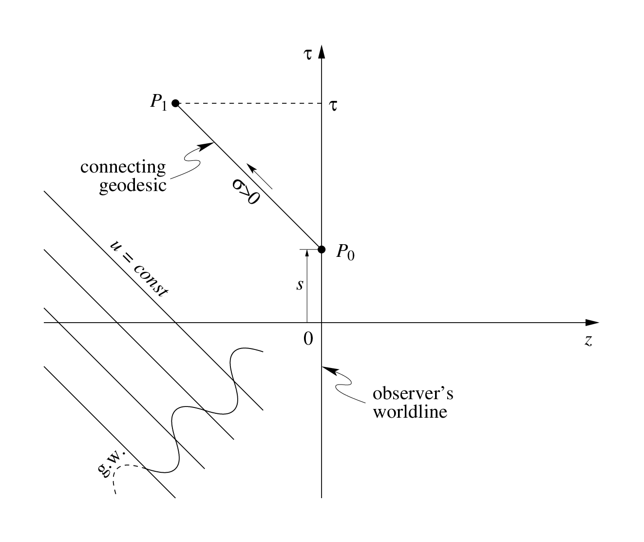
As before, we assume that the connecting geodesic originates from the worldline of the observer, at point $P_{0}=\{s,0,0,0\}$ , and ends at an arbitrary point in this spacetime, $P_{1}=\{\tau,x,y,z\}$ . The affine parameter along the geodesic takes the value $\sigma=0$ at point $P_{0}$ and $\sigma=\sigma_{1}$ at point $P_{1}$ . The solution for the geodesic equation (Section 3.4) connects the coordinates of points $P_{0}$ and $P_{1}$ :

$\displaystyle x$	$\displaystyle=$	$\displaystyle p_{x0}\,\sigma_{1}\,(1-h_{+})-p_{y0}\,\sigma_{1}\,h_{\times},$	(213)
$\displaystyle y$	$\displaystyle=$	$\displaystyle p_{y0}\,\sigma_{1}\,(1+h_{+})-p_{x0}\,\sigma_{1}\,h_{\times},$	(214)
$\displaystyle z$	$\displaystyle=$	$\displaystyle A\sigma_{1}^{2}+B\sigma_{1},$	(215)
$\displaystyle\tau$	$\displaystyle=$	$\displaystyle s-A\sigma_{1}^{2}-B\sigma_{1},$	(216)

where $h_{a}$ is constant along the geodesic:

h_{a}=h_{a}(u)=h_{a}(u_{0}).

(217)

The boundary value problem is to determine arbitrary constants $p_{x0},p_{y0},A,B,s$ , $\sigma_{1}$ in terms of the coordinates of point $P_{1}$ .

First, we find parameter $s$ a function of the coordinates of $P_{1}$ . By definition, $s=u_{0}$ . Since $u$ is constant along the geodesic (212), we find that

s=u,\qquad{\mathrm{or}}\qquad s=\tau+z.

(218)

Second, inverting (213) and (214) to first order in $h$ , we obtain

	$\displaystyle p_{x0}$	$\displaystyle=$	$\displaystyle(1+h_{+})\frac{x}{\sigma_{1}}+h_{\times}\,\frac{y}{\sigma_{1}},$		(219)
	$\displaystyle p_{y0}$	$\displaystyle=$	$\displaystyle(1-h_{+})\frac{y}{\sigma_{1}}+h_{\times}\,\frac{x}{\sigma_{1}}.$		(220)

Substituting these equations in the normalization condition (29) with $\epsilon=1$ , we obtain the formula for $\sigma_{1}$ :

\sigma_{1}^{2}=x^{2}+y^{2}+(x^{2}-y^{2})h_{+}+2xy\,h_{\times}.

(221)

Naturally, there are two solutions:

\sigma_{1}=\pm\left[x^{2}+y^{2}+(x^{2}-y^{2})h_{+}+2xy\,h_{\times}\right]^{1/2}.

(222)

The solution with the “ $-$ ” sign corresponds to another singular geodesic with the same parameter $u_{0}$ . This second geodesic connects $P_{0}$ with point $P_{2}=\{\tau,-x,-y,z\}$ which is the inverse of point $P_{1}$ in the $xy$ -plane. Therefore, we can safely discard this solution. Taking the “ $+$ ” sign and keeping only terms first order in $h$ , we obtain the final solution for $\sigma_{1}$ :

\sigma_{1}\approx\rho+\frac{1}{2\rho}\left[(x^{2}-y^{2})\,h_{+}+2xy\,h_{\times}\right],

(223)

where $\rho=\sqrt{x^{2}+y^{2}}$ .

Next, we can substitute $p_{x0}$ and $p_{y0}$ in (56) and find the constant $A$ to first order in $h$ :

A=\frac{1}{4\sigma_{1}^{2}}\left[(x^{2}-y^{2})h^{\prime}_{+}+2xy\,h^{\prime}_{\times}\right].

(224)

Knowing $A$ and $\sigma_{1}$ , we can find $B$ from (215),

B=\frac{1}{\sigma_{1}}\left(z-A\sigma_{1}^{2}\right).

(225)

It follows from equations (215) and (216) that

\left.p^{z}\right|_{\sigma=0}=-\left.p^{\tau}\right|_{\sigma=0}=B.

(226)

We now turn to the derivation of the coordinate transformation rules using the definition (99). Consider first the $x$ coordinate:

	$\displaystyle\bar{x}$	$\displaystyle\equiv$	$\displaystyle\lambda^{\bar{x}x}p_{x0}\sigma_{1}+\lambda^{\bar{x}y}p_{y0}\sigma_{1}$		(227)
		$\displaystyle=$	$\displaystyle x+\frac{1}{2}x\,h_{+}+\frac{1}{2}y\,h_{\times}.$		(227)

Similarly, we derive the transformation rule for the $y$ coordinate:

	$\displaystyle\bar{y}$	$\displaystyle\equiv$	$\displaystyle\lambda^{\bar{y}y}p_{y0}\sigma_{1}+\lambda^{\bar{y}x}p_{x0}\sigma_{1}$		(228)
		$\displaystyle=$	$\displaystyle y-\frac{1}{2}y\,h_{+}+\frac{1}{2}x\,h_{\times}.$		(228)

Using (226), we can obtain a formula for $z$ ,

$\displaystyle\bar{z}$	$\displaystyle\equiv$	$\displaystyle\lambda^{\bar{z}}{}_{z}\left.p^{z}\right\|_{\sigma=0}\sigma_{1}$	(229)
	$\displaystyle=$	$\displaystyle B\sigma_{1}$
	$\displaystyle=$	$\displaystyle z-A\sigma_{1}^{2},$

and for $\tau$ ,

$\displaystyle\bar{\tau}$	$\displaystyle\equiv$	$\displaystyle s+\lambda^{\bar{\tau}}{}_{\tau}\left.p^{\tau}\right\|_{\sigma=0}\sigma_{1}$	(230)
	$\displaystyle=$	$\displaystyle s-B\sigma_{1}$
	$\displaystyle=$	$\displaystyle\tau+A\sigma_{1}^{2}.$

We have thus obtained the transformation rules for wave-synchronous coordinates, which can be summarized as

$\displaystyle\bar{x}$	$\displaystyle=$	$\displaystyle x+\frac{1}{2}x\,h_{+}(u)+\frac{1}{2}y\,h_{\times}(u),$	(231)
$\displaystyle\bar{y}$	$\displaystyle=$	$\displaystyle y-\frac{1}{2}y\,h_{+}(u)+\frac{1}{2}x\,h_{\times}(u),$	(232)
$\displaystyle\bar{z}$	$\displaystyle=$	$\displaystyle z-\frac{1}{4}(x^{2}-y^{2})h^{\prime}_{+}(u)-\frac{1}{2}xyh^{\prime}_{\times}(u),$	(233)
$\displaystyle\bar{\tau}$	$\displaystyle=$	$\displaystyle\tau+\frac{1}{4}(x^{2}-y^{2})h^{\prime}_{+}(u)+\frac{1}{2}xyh^{\prime}_{\times}(u).$	(234)

Equivalently, one can use $u,v$ instead of $z,\tau$ :

	$\displaystyle\bar{u}$	$\displaystyle=$	$\displaystyle u,$		(235)
	$\displaystyle\bar{v}$	$\displaystyle=$	$\displaystyle v+\frac{1}{2}(x^{2}-y^{2})h^{\prime}_{+}(u)+xyh^{\prime}_{\times}(u).$		(236)

To find the metric in wave-synchronous coordinates we need to invert the coordinate transformation rules, equations (231), (232), (235), (236) and substitute the resulting formulae in the fundamental form (21). The result is

F=-\rmd\bar{u}\,\rmd\bar{v}+\rmd\bar{x}^{2}+\rmd\bar{y}^{2}-2\Phi\rmd\bar{u}^{2},

(237)

where $\Phi$ is given by

\Phi=-\frac{1}{4}(\bar{x}^{2}-\bar{y}^{2})\,h^{\prime\prime}_{+}(\bar{u})-\frac{1}{2}\bar{x}\bar{y}\,h^{\prime\prime}_{\times}(\bar{u}).

(238)

Therefore, the nonzero components of the metric in wave-synchronous coordinates are

$\displaystyle\bar{g}_{xx}$	$\displaystyle=$	$\displaystyle 1,$	(239)
$\displaystyle\bar{g}_{yy}$	$\displaystyle=$	$\displaystyle 1,$	(240)
$\displaystyle\bar{g}_{zz}$	$\displaystyle=$	$\displaystyle 1-2\Phi,$	(241)
$\displaystyle\bar{g}_{\tau z}$	$\displaystyle=$	$\displaystyle-2\Phi,$	(242)
$\displaystyle\bar{g}_{\tau\tau}$	$\displaystyle=$	$\displaystyle-1-2\Phi.$	(243)

This metric represents the exact solution of the Einstein equations found by Peres [19] and also by Ehlers and Kundt [20]. The equivalence of the exact solution and the metric of the wave-synchronous coordinates was previously discussed in [18].

We have seen that Fermi normal coordinates are valid for arbitrarily large distances in the longitudinal ( $\bar{z}$ ) direction but are limited in the transverse ( $\bar{x}\bar{y}$ ) plane. Since wave-synchronous coordinates correspond to the exact solution of general relativity, they are not restricted in space the way Fermi normal coordinates are. The exact solution requires special attention in the case when $|\Phi|\sim 1$ for which $\bar{g}_{\tau\tau}$ may vanish. Analysis of the metric in this regime belongs to the study of exact solutions of general relativity and is outside the scope of this paper.

9 Comparison of the coordinate systems

In this Section, we briefly consider how the different coordinate systems can be used to describe the motion of an inertial test mass which is placed in the field of a gravitational wave. In what follows, the normal coordinates will appear as $x,y,z,\tau$ , i.e. without the overline, for simplicity.

9.1 TT gauge versus normal coordinates

As we have seen in Section 4, an inertial test mass that is initially at rest in the TT coordinate system will remain at rest even in the presence of a gravitational wave. Here the words “at rest” only mean that the coordinates of the test mass are not changing. One way to realize such a coordinate system would be to use inertial masses themselves to define the coordinate grid. Imagine a large number of inertial masses in space forming a 3-dimensional cubic lattice and assume that initially no mass is moving relative to the other. For any point on the grid, its order numbers along the three lattice dimensions would yield the TT coordinates of that location. Assume that a test mass is introduced in this space, and it is at rest with respect to this grid. Then there will be no relative motion between the test mass and the co-located mass on the grid even in the presence of a gravitational wave. Therefore, the coordinates of the test mass will not be changing. However, the proper distance between any two masses on the grid will be changing due to changes in the metric that are caused by the gravitational wave. An effort to make changes in the proper distance between two masses appear as changes in their coordinates would lead to normal coordinate construction. In a normal coordinate system, an inertial test mass will appear to be moving with respect to the coordinate grid, i.e. its coordinates will be changing. The details of this motion will depend on the type of the normal coordinates used. We consider here the motion of an inertial test mass under the influence of a gravitational wave for two normal coordinate systems described above: Fermi and wave-synchronous.

9.2 Motion of a test mass in Fermi normal coordinates

If the test mass was at rest in TT coordinates, it will be moving in FN coordinates. The exact dependence of the test mass coordinates on time is given by equations (113)–(116) in which we have to assume that the TT coordinates are constant. In FN coordinates, the test mass is experiencing acceleration which indicates the presence of forces produced by the gravitational wave. To analyze these forces we need to find explicit formulae for the acceleration of the test mass. Differentiating equations (113)–(116) twice with respect to time and replacing the constant TT coordinates with their FN counterparts, we obtain

$\displaystyle\frac{\rmd^{2}x}{\rmd\tau^{2}}$	$\displaystyle=$	$\displaystyle\frac{1}{2}x\,h^{\prime\prime}_{+}+\frac{1}{2}y\,h^{\prime\prime}_{\times}+z\left(x\,H^{\prime\prime}_{+}+yH^{\prime\prime}_{\times}\right),$	(244)
$\displaystyle\frac{\rmd^{2}y}{\rmd\tau^{2}}$	$\displaystyle=$	$\displaystyle\frac{1}{2}x\,h^{\prime\prime}_{\times}-\frac{1}{2}y\,h^{\prime\prime}_{+}+z\left(x\,H^{\prime\prime}_{\times}-y\,H^{\prime\prime}_{+}\right),$	(245)
$\displaystyle\frac{\rmd^{2}z}{\rmd\tau^{2}}$	$\displaystyle=$	$\displaystyle-\frac{1}{2}(x^{2}-y^{2})H^{\prime\prime}_{+}-xyH^{\prime\prime}_{\times},$	(246)

where primes denote derivatives with respect to $\tau$ . The function $H_{a}$ was introduced in (112) and its derivatives

	$\displaystyle H^{\prime}_{a}$	$\displaystyle=$	$\displaystyle\frac{1}{z^{2}}\left[h_{a}(\tau+z)-h_{a}(\tau)-zh^{\prime}_{a}(\tau)\right],$		(247)
	$\displaystyle H^{\prime\prime}_{a}$	$\displaystyle=$	$\displaystyle\frac{1}{z^{2}}\left[h^{\prime}_{a}(\tau+z)-h^{\prime}_{a}(\tau)-zh^{\prime\prime}_{a}(\tau)\right],$		(248)

are finite in the limit of $z\rightarrow 0$ .

One can also find the test mass acceleration directly in FN coordinates, bypassing the TT gauge altogether. Indeed, taking the equations for a geodesic in FN coordinates,

\frac{\rmd^{2}x^{i}}{\rmd\tau^{2}}=\frac{1}{2}\frac{\partial C_{\tau\tau}}{\partial x^{i}}-\frac{\partial C_{\tau i}}{\partial\tau},\qquad{\mathrm{for}}\qquad i=1,2,3,

(249)

and substituting in them the formulae for the metric coefficients $C_{\tau i}$ and $C_{\tau\tau}$ from (135)–(138) we can obtain equations (244)–(246). These equations describe the acceleration of the test mass in response to the propagating gravitational wave. In this form, they are not easy to interpret. We know for example, that the longitudinal acceleration (along $z$ ) is much smaller than the acceleration in the transverse directions ( $x,y$ ) but this is not obvious from these equations.

Interpretation of the acceleration will be straightforward if the equations are presented in the Newtonian form. This can be done as follows. First, we replace $\tau$ with $t$ via $\tau=ct$ . Then we introduce the scalar field $\phi$ and the vector field ${\mathbf{b}}$ according to the definitions:

	$\displaystyle C_{\tau\tau}$	$\displaystyle=$	$\displaystyle-\frac{2}{c^{2}}\phi,$		(250)
	$\displaystyle C_{\tau i}$	$\displaystyle=$	$\displaystyle-\frac{1}{c^{2}}b_{i}.$		(251)

With these notational changes, equations (249) can be written in the Newtonian form:

\frac{\rmd^{2}{\mathbf{r}}}{\rmd t^{2}}=-\nabla\phi+\frac{1}{c}\frac{\partial{\mathbf{b}}}{\partial t}.

(252)

Here $\phi$ represents the dominant part of the acceleration produced by the gravitational wave and ${\mathbf{b}}$ generates relativistic corrections. (The relativistic corrections come from both $\phi$ and ${\mathbf{b}}$ , but only $\phi$ generates the non-relativistic part.)

Explicit formula for the scalar field can be found from (138),

\phi=-\frac{c^{2}}{2z^{2}}\left[(x^{2}-y^{2})\left(2Q_{+}-P_{+}\right)+2xy\left(2Q_{\times}-P_{\times}\right)\right].

(253)

Explicit formulae for the vector field can be found from (135) – (137),

$\displaystyle b_{x}$	$\displaystyle=$	$\displaystyle\frac{c^{2}}{z}\left(xQ_{+}+yQ_{\times}\right),$	(254)
$\displaystyle b_{y}$	$\displaystyle=$	$\displaystyle\frac{c^{2}}{z}\left(xQ_{\times}-yQ_{+}\right),$	(255)
$\displaystyle b_{z}$	$\displaystyle=$	$\displaystyle-\frac{c^{2}}{z^{2}}\left[(x^{2}-y^{2})Q_{+}+2xyQ_{\times}\right].$	(256)

Note that equation (253) can also be written as

\phi=-\frac{c^{2}}{2}\left[(x^{2}-y^{2})H^{\prime}_{+}+2xyH^{\prime}_{\times}\right],

(257)

where $H_{a}^{\prime}$ is given by (247).

The non-relativistic approximation of (252) can be obtained by expanding scalar field $\phi$ and vector field ${\mathbf{b}}$ in powers of $1/c$ . The leading terms in this expansion are given by the second-order approximation for the metric, (161)–(164). We will also need to make the substitution:

h_{a}(\tau+z)=\eta_{a}\left(t+\frac{z}{c}\right),

(258)

which will allow expansion of $h_{a}$ in powers of $1/c$ . Consistency requires that we expand $\phi$ to the first order:

\phi=\phi_{0}+\phi_{1},

(259)

where $\phi_{0}$ is purely non-relativistic and $\phi_{1}$ is of order $1/c$ . Consider first the non-relativistic part of the potential $\phi_{0}$ . Taking the leading (zeroth-order) terms in the expansion of $H_{a}$ in (257) we find that

\phi_{0}=-\frac{1}{4}(x^{2}-y^{2})\ddot{\eta}_{+}(t)-\frac{1}{2}xy\,\ddot{\eta}_{\times}(t).

(260)

This part defines the non-relativistic approximation for the test mass acceleration:

$\displaystyle-\frac{\partial\phi_{0}}{\partial x}$	$\displaystyle=$	$\displaystyle\frac{1}{2}x\,\ddot{\eta}_{+}(t)+\frac{1}{2}y\,\ddot{\eta}_{\times}(t),$	(261)
$\displaystyle-\frac{\partial\phi_{0}}{\partial y}$	$\displaystyle=$	$\displaystyle\frac{1}{2}x\,\ddot{\eta}_{\times}(t)-\frac{1}{2}y\,\ddot{\eta}_{+}(t),$	(262)
$\displaystyle-\frac{\partial\phi_{0}}{\partial z}$	$\displaystyle=$	$\displaystyle 0.$	(263)

In this picture, the gravitational wave manifests itself through the time-dependent potential which generates the forces acting on the mass (one for each polarization $+$ and $\times$ ). These forces are orthogonal to the direction of the gravitational-wave propagation. Therefore, the motion of the test mass caused by these forces is confined to the transverse plane.

In the non-relativistic approximation, the scalar field satisfies the Laplace equation

\nabla^{2}\phi_{0}=0.

(264)

The same equation is satisfied by gravitational potentials away from the sources in Newtonian physics. In this regard, the scalar field can be viewed as a special case of a gravitational potential.

The relativistic corrections come from $\phi_{1}$ and ${\mathbf{b}}$ . Taking the first-order terms in the expansion of $H_{a}$ in (257) we find that

\phi_{1}=-\frac{1}{12c}z\left[(x^{2}-y^{2}){\eta}^{(3)}_{+}(t)+2xy\,{\eta}^{(3)}_{\times}(t)\right].

(265)

Expanding (161)–(163) in powers of $1/c$ and keeping the leading order terms, we obtain

$\displaystyle b_{x}$	$\displaystyle=$	$\displaystyle\frac{1}{3}z\left[x\,\ddot{\eta}_{+}(t)+y\,\ddot{\eta}_{\times}(t)\right],$	(266)
$\displaystyle b_{y}$	$\displaystyle=$	$\displaystyle\frac{1}{3}z\left[x\,\ddot{\eta}_{\times}(t)-y\,\ddot{\eta}_{+}(t)\right],$	(267)
$\displaystyle b_{z}$	$\displaystyle=$	$\displaystyle-\frac{1}{3}\left[(x^{2}-y^{2})\ddot{\eta}_{+}(t)+2xy\,\ddot{\eta}_{\times}(t)\right].$	(268)

Thus, the first-order relativistic correction to the test mass acceleration is given by

$\displaystyle-\frac{\partial\phi_{1}}{\partial x}+\frac{1}{c}\frac{\partial b_{x}}{\partial t}$	$\displaystyle=$	$\displaystyle\frac{1}{2c}z\left[x\,\eta^{(3)}_{+}(t)+y\,\eta^{(3)}_{\times}(t)\right],$	(269)
$\displaystyle-\frac{\partial\phi_{1}}{\partial y}+\frac{1}{c}\frac{\partial b_{y}}{\partial t}$	$\displaystyle=$	$\displaystyle\frac{1}{2c}z\left[x\,\eta^{(3)}_{\times}(t)-y\,\eta^{(3)}_{+}(t)\right],$	(270)
$\displaystyle-\frac{\partial\phi_{1}}{\partial z}+\frac{1}{c}\frac{\partial b_{z}}{\partial t}$	$\displaystyle=$	$\displaystyle-\frac{1}{4c}\left[(x^{2}-y^{2})\,\eta^{(3)}_{+}(t)+2xy\,\eta^{(3)}_{\times}(t)\right].$	(271)

We conclude by noting that vector field ${\mathbf{b}}$ in the non-relativistic approximation, (266)–(268), is divergence free,

\nabla\cdot{\mathbf{b}}=0.

(272)

This means that there is a vector field ${\mathbf{a}}$ such that

{\mathbf{b}}=\nabla\times{\mathbf{a}}.

(273)

The definition of ${\mathbf{a}}$ is not unique. Here we give one possible realization for this vector field:

$\displaystyle a_{x}$	$\displaystyle=$	$\displaystyle\frac{1}{3}x^{2}y\,\ddot{\eta}_{+}(t)+\frac{1}{6}xy^{2}\,\ddot{\eta}_{\times}(t),$	(274)
$\displaystyle a_{y}$	$\displaystyle=$	$\displaystyle\frac{1}{3}xy^{2}\,\ddot{\eta}_{+}(t)-\frac{1}{6}x^{2}y\,\ddot{\eta}_{\times}(t),$	(275)
$\displaystyle a_{z}$	$\displaystyle=$	$\displaystyle\frac{1}{3}xyz\,\ddot{\eta}_{+}(t)-\frac{1}{6}z(x^{2}-y^{2})\ddot{\eta}_{\times}(t),$	(276)

which can be useful for calculations of the motion of continuous media (fluids or elastic bodies) in the presence of a gravitational wave.

Note that the dependence of the potential $\phi$ on $z$ and $t$ is not consistent with the relativistic form of the gravitational-wave propagation, e.g. (258). The same is true for the vector field ${\mathbf{b}}$ in which $z$ and $t$ are not related in any way. This problem does not occur in wave-synchronous coordinate system, as we will see next.

9.3 Motion of a test mass in wave-synchronous coordinates

The description of test mass motion in wave-synchronous coordinates is similar to the description in Fermi normal coordinates. In wave-synchronous coordinates, the test mass will be moving under the influence of the gravitational wave. The exact dependence of the test mass coordinates on time is given by equations (231)–(233) in which we have assume that the TT coordinates are constant. To analyze the forces acting on the test mass we need to find the explicit formulae for its acceleration. Differentiating equations (231)–(233) twice with respect to time and replacing the constant TT coordinates with their wave-synchronous counterparts, we obtain

$\displaystyle\frac{\rmd^{2}x}{\rmd\tau^{2}}$	$\displaystyle=$	$\displaystyle\frac{1}{2}x\,h^{\prime\prime}_{+}(u)+\frac{1}{2}y\,h^{\prime\prime}_{\times}(u),$	(277)
$\displaystyle\frac{\rmd^{2}y}{\rmd\tau^{2}}$	$\displaystyle=$	$\displaystyle\frac{1}{2}x\,h^{\prime\prime}_{\times}(u)-\frac{1}{2}y\,h^{\prime\prime}_{+}(u),$	(278)
$\displaystyle\frac{\rmd^{2}z}{\rmd\tau^{2}}$	$\displaystyle=$	$\displaystyle-\frac{1}{4}(x^{2}-y^{2})h^{\prime\prime\prime}_{+}(u)-\frac{1}{2}xy\,h^{\prime\prime\prime}_{\times}(u),$	(279)

where primes denote derivatives with respect to $u$ .

One can find the test mass acceleration directly in wave-synchronous coordinates, bypassing the TT gauge altogether. Indeed, taking the equations for a geodesic in wave-synchronous coordinates [18],

\frac{\rmd^{2}x^{i}}{\rmd\tau^{2}}=\frac{1}{2}\frac{\partial g_{\tau\tau}}{\partial x^{i}}-\frac{\partial g_{\tau i}}{\partial\tau},\qquad{\mathrm{for}}\qquad i=1,2,3,

(280)

and substituting in them the formulae for the metric coefficients $g_{\tau i}$ and $g_{\tau\tau}$ from (242) and (243), we can obtain equations (277)–(279).

By replacing $\tau$ with $t$ and introducing the scalar and vector fields,

	$\displaystyle 1+g_{\tau\tau}$	$\displaystyle=$	$\displaystyle-\frac{2}{c^{2}}\phi,$		(281)
	$\displaystyle g_{\tau i}$	$\displaystyle=$	$\displaystyle-\frac{1}{c^{2}}b_{i},$		(282)

we can present equations (280) in the Newtonian form:

\frac{\rmd^{2}{\mathbf{r}}}{\rmd t^{2}}=-\nabla\phi+\frac{1}{c}\frac{\partial{\mathbf{b}}}{\partial t}.

(283)

Here $\phi$ represents the dominant part of the acceleration produced by the gravitational wave and ${\mathbf{b}}$ generates relativistic corrections. In the explicit form, the scalar field is given by

\phi=-\frac{1}{4}(x^{2}-y^{2})\,\ddot{\eta}_{+}\left(t+\frac{z}{c}\right)-\frac{1}{2}xy\,\ddot{\eta}_{\times}\left(t+\frac{z}{c}\right).

(284)

The vector field has the following components:

$\displaystyle b_{x}$	$\displaystyle=$	$\displaystyle 0,$	(285)
$\displaystyle b_{y}$	$\displaystyle=$	$\displaystyle 0,$	(286)
$\displaystyle b_{z}$	$\displaystyle=$	$\displaystyle 2\phi.$	(287)

The scalar field $\phi$ plays the role of the potential which generates the forces acting on the test mass. Note that in wave-synchronous coordinates the potential acquires the full $z$ -dependence consistent with the relativistic nature of the gravitational wave. This can also be seen from the fact that the potential satisfies the wave equation:

\nabla^{2}\phi=\frac{1}{c^{2}}\frac{\partial^{2}\phi}{\partial t^{2}}.

(288)

One can think of this potential as the fully relativistic version of the potential in Fermi normal coordinates.

Consider now the vector field ${\mathbf{b}}$ . In wave-synchronous coordinates ${\mathbf{b}}$ produces a purely longitudinal acceleration of the test mass. In fact, it is equal to twice the acceleration produced by the potential (in the opposite direction):

\frac{1}{c}\frac{\partial b_{z}}{\partial t}=2\frac{\partial\phi}{\partial z}.

(289)

Also note that vector field ${\mathbf{b}}$ is not divergence free. Instead, it satisfies

\nabla\cdot{\mathbf{b}}=\frac{2}{c}\frac{\partial\phi}{\partial t}.

(290)

This equation can be written in the covariant 4-dimensional form:

\partial_{\mu}b^{\mu}\equiv-\partial_{\tau}b_{\tau}+\nabla\cdot{\mathbf{b}}=0,

(291)

where 4-vector $b_{\mu}$ is formed from ${\mathbf{b}}$ by adding the time component, $b_{\tau}=2\phi$ . Therefore,

b_{\mu}=\{2\phi,0,0,2\phi\}.

(292)

Another way to introduce the 4-vector $b_{\mu}$ is through the metric tensor:

g_{\tau\mu}=\eta_{\tau\mu}-\frac{1}{c^{2}}b_{\mu},

(293)

where $g_{\tau\mu}$ are the components of the metric in wave-synchronous coordinates.

The non-relativistic approximation for the test mass acceleration can be found by expanding (284) in powers of $1/c$ . It is interesting to note that the zeroth and the first order approximations for the acceleration in wave-synchronous coordinates are identical to those in Fermi normal coordinates. The advantage of wave-synchronous coordinate system is that it allows us to have the acceleration to all orders in $1/c$ and provides a mathematical formalism which is fully consistent with the relativistic nature of the gravitational wave.

10 Conclusion

Normal coordinates are a convenient tool for analysis of the effects of gravitational waves from the point of view of an inertial observer. We have revisited the normal-coordinate construction for a plane gravitational wave and showed that it depends on the boundary-value problem for the connecting geodesic. Three different types of the boundary-value problem have been considered in this paper. The first is based on a non-singular spacelike connecting geodesic that is orthogonal to the observer’s worldline. This construction leads to Fermi normal coordinates. The second boundary-value problem is based on a null connecting geodesic and leads to optical coordinates. The third is based on a singular spacelike connecting geodesic and leads to wave-synchronous coordinates. For each type of the boundary-value problem we obtained explicit formulae for the coordinate transformation rules and the induced metric. These formulae are exact as long as the calculations stay within the linearized theory of gravitation. In particular, they are valid for arbitrarily large distances in the longitudinal direction. Also, we showed that the exact formulae yield the infinite-series representation for Fermi normal coordinates and the induced metric. We have thus found that the infinite series for FN coordinates and the induced metric can actually be summed and the result of this summation can be given in a closed analytical form.

Historically, Fermi-normal coordinates have always been limited to the long-wavelength regime. However, as we have shown, Fermi normal coordinates can actually be defined far beyond the long-wavelength regime. No change in point of view and no transition of any kind occurs at distances equal to or comparable with the wavelength of the gravitational wave. We can now conclude that the range limitation that has always been associated with Fermi normal coordinates was rather unnecessary. Without this limitation, Fermi normal coordinates become a viable alternative to the TT coordinates for theoretical studies of gravitational waves. We also found that wave-synchronous coordinates yield the exact solution of Peres and Ehlers-Kundt. Since this solution is globally defined, the system of wave-synchronous coordinates is valid for arbitrarily large distances. This was possible due to the special geometry of spacetime which represents a plane gravitational wave propagating in a flat background.

I would like to thank many people with whom I discussed this work, particularly Kip Thorne who stressed the importance of these calculations at the beginning of this research, and also Joe Romano and the late Leonid Grishchuk with whom I had many interesting conversations about the role of the coordinate system in the detector response near the end of this work. In addition, I would like to thank Rick Savage and Joe Romano for comments on the final version of the paper, and Anton Gribovskiy for verifying the calculations of the induced metric. This paper took a long time to mature. The work started at the Center for Gravitational Wave Physics at Penn State, continued at the LIGO Hanford Observatory, and was finished at the Center for Gravitational Wave Astronomy at the University of Texas at Brownsville. At Penn State, this research was supported by the US National Science Foundation under grants PHY 00-99559, 02-44902, 03-26281, and 06-00953. At LIGO, it was supported by a Visiting Research Fellowship from Caltech. At Brownsville, it was supported by the US National Science Foundation under grants HRD 0734800 and 1242090, and by the US NASA University Research Centers under grant NNX 09AV06A. The first version of this paper was circulated within the LIGO Scientific Collaboration in 2006. This paper has been assigned LIGO Document Number P060066.

References

[1] Fermi E 1922 Atti R. Accad. Lincei Rend. Cl. Sci. Fis. Mat. Nat. 31 21, 51
[2] O’Raifeartaigh L 1958 Proc. Roy. Irish Acad. 59A 15
[3] Synge J 1960 Relativity: The General Theory (Amsterdam: North-Holland Publishing Co.)
[4] Manasse F and Misner C 1963 J. Math. Phys. 4 735
[5] Ni W T and Zimmermann M 1978 Phys. Rev.D 17 1473
[6] Weber J 1961 General Relativity and Gravitational Waves (New York: Interscience Publishers, Inc.)
[7] Misner C, Thorne K and Wheeler J 1973 Gravitation (San Francisco: W.H. Freeman and Co.)
[8] Rakhmanov M, Romano J and Whelan J 2008 Class. Quantum Grav. 25 184017
[9] Grishchuk L 1977 Sov. Phys. Usp. 20 319
[10] Grishchuk L and Polnarev A 1980 in A Held, ed, General Relativity and Gravitation: One hundred years after the birth of Albert Einstein vol 2 (New York: Plenum Press) pp 393–434
[11] Pegoraro F, Picasso E and Radicati L 1978 J. Phys. A: Math. Gen. 11 1949
[12] Fortini P and Gualdi C 1982 Nuovo Cimento 71 B 37
[13] Flores G and Orlandini M 1986 Nuovo Cimento 91 B 236
[14] Callegari G, Fortini P and Gualdi C 1987 Nuovo Cimento 100 B 421
[15] Fortini P and Ortolan A 1990 in R Cherubini, P Dalpiaz and B Minetti, eds, Problems of fundamental modern physics: proceedings of the 4th Winter School on Hadronic Physics (Folgaria (Trento), Italy: World Scientific) pp 468–478
[16] Fortini P and Ortolan A 1991 Nuovo Cimento(Note Brevi) 106 B 101
[17] Baskaran D and Grishchuk L 2004 Class. Quantum Grav. 21 4041
[18] Rakhmanov M 2005 Phys. Rev.D 71 084003
[19] Peres A 1959 Phys. Rev. Lett. 3 571
[20] Ehlers J and Kundt W 1962 in L Witten, ed, Gravitation: an introduction to current research (New York, London: John Wiley & Sons, Inc.) pp 49–101
[21] Li W Q and Ni W T 1979 J. Math. Phys. 20 1473
[22] Li W Q and Ni W T 1979 J. Math. Phys. 20 1925
[23] Marzlin K P 1994 Phys. Rev.D 50 888
[24] Rakhmanov M 2009 Class. Quantum Grav. 26 155010

Appendix A Christoffel coefficients and Riemann tensor

In the linearized theory of gravitation Christoffel coefficients are given by

\Gamma_{\alpha\beta\gamma}=\frac{1}{2}\left(h_{\alpha\beta,\gamma}+h_{\alpha\gamma,\beta}-h_{\beta\gamma,\alpha}\right).

(294)

For the metric defined in (21), $h_{\alpha\beta}$ depends essentially on one coordinate:

h_{\alpha\beta}=h_{\alpha\beta}(u),\qquad{\mathrm{where}}\qquad u=\tau+z.

(295)

Then the non-zero independent Christoffel coefficients are

	$\displaystyle\Gamma_{xxu}=-\Gamma_{uxx}=-\Gamma_{yyu}=\Gamma_{uyy}=\frac{1}{2}\,h^{\prime}_{+}(u),$		(296)
	$\displaystyle\Gamma_{xyu}=-\Gamma_{uxy}=\Gamma_{yxu}=\frac{1}{2}\,h^{\prime}_{\times}(u),$		(297)

where primes stand for differentiation with respect to $u$ . Switching from $u,v$ to $\tau,z$ , we find

	$\displaystyle\Gamma_{xx\tau}=-\Gamma_{\tau xx}=\Gamma_{xxz}=-\Gamma_{zxx}=\frac{1}{2}\,h^{\prime}_{+}(\tau+z),$		(298)
	$\displaystyle\Gamma_{yy\tau}=-\Gamma_{\tau yy}=\Gamma_{yyz}=-\Gamma_{zyy}=-\frac{1}{2}\,h^{\prime}_{+}(\tau+z),$		(299)
	$\displaystyle\Gamma_{xy\tau}=-\Gamma_{\tau xy}=\Gamma_{yx\tau}=\frac{1}{2}\,h^{\prime}_{\times}(\tau+z),$		(300)
	$\displaystyle\Gamma_{xyz}=-\Gamma_{zxy}=\Gamma_{yxz}=\frac{1}{2}\,h^{\prime}_{\times}(\tau+z),$		(301)

where primes stand for differentiation with respect to $z$ or $\tau$ .

The components of the Riemann tensor [7] are defined according to

R^{\mu}{}_{\nu\alpha\beta}=\Gamma^{\mu}{}_{\nu\beta,\alpha}-\Gamma^{\mu}{}_{\nu\alpha,\beta}+\Gamma^{\mu}{}_{\rho\alpha}\Gamma^{\rho}{}_{\nu\beta}-\Gamma^{\mu}{}_{\rho\beta}\Gamma^{\rho}{}_{\nu\alpha}.

(302)

In the linearized theory, this definition reduces to

R_{\mu\nu\alpha\beta}=\Gamma_{\mu\nu\beta,\alpha}-\Gamma_{\mu\nu\alpha,\beta}.

(303)

Substituting for Christoffel coefficients from (294), we obtain

R_{\mu\nu\alpha\beta}=\frac{1}{2}(h_{\mu\beta,\nu\alpha}-h_{\mu\alpha,\nu\beta}+h_{\nu\alpha,\mu\beta}-h_{\nu\beta,\mu\alpha}).

(304)

There are only three non-zero independent components of the Riemann tensor corresponding to metric defined in (21):

	$\displaystyle R_{xuxu}=R_{yuyu}=-\frac{1}{2}\,h^{\prime\prime}_{+}(u),$		(305)
	$\displaystyle R_{xuyu}=-\frac{1}{2}\,h^{\prime\prime}_{\times}(u).$		(306)

Switching from $u,v$ to $\tau,z$ , we find

	$\displaystyle R_{x\tau x\tau}=R_{x\tau xz}=R_{xzxz}=-\frac{1}{2}\,h^{\prime\prime}_{+}(\tau+z),$		(307)
	$\displaystyle R_{y\tau y\tau}=R_{y\tau yz}=R_{yzyz}=\frac{1}{2}\,h^{\prime\prime}_{+}(\tau+z),$		(308)
	$\displaystyle R_{x\tau y\tau}=R_{x\tau yz}=R_{xzy\tau}=R_{xzyz}=-\frac{1}{2}\,h^{\prime\prime}_{\times}(\tau+z).$		(309)