跳到论文正文
W Papers独立论文阅读器 arXiv:1409.4639 论文正文 计算阅读时间 · 0%
引用这篇论文根据当前论文元数据生成,正式投稿前建议核对。


License: arXiv.org perpetual non-exclusive license
arXiv:1409.4639v1 [eess.SY] 16 Sep 2014

Ultimate Boundedness of Droop Controlled Microgrids
with Secondary Loops

Rahmat Heidari Affiliation:  Priority Research Centre for Complex Dynamic Systems and Control (CDSC), School of Electrical Engineering and Computer Science, The University of Newcastle, Callaghan NSW 2308, Australia heidari.rahmat@gmail.com, maria.seron@newcastle.edu.au    Maria M. Seron Affiliation:  Priority Research Centre for Complex Dynamic Systems and Control (CDSC), School of Electrical Engineering and Computer Science, The University of Newcastle, Callaghan NSW 2308, Australia heidari.rahmat@gmail.com, maria.seron@newcastle.edu.au    Julio H. Braslavsky Affiliation:  Australian Commonwealth Scientific and Industrial Research Organisation (CSIRO), Energy Flagship, PO box 330, Newcastle, NSW 2300, Australia julio.braslavsky@csiro.au
Abstract

In this paper we study theoretical properties of inverter-based microgrids controlled via primary and secondary loops. Stability of these microgrids has been the subject of a number of recent studies. Conventional approaches based on standard hierarchical control rely on time-scale separation between primary and secondary control loops to show local stability of equilibria. In this paper we show that (i) frequency regulation can be ensured without assuming time-scale separation and, (ii) ultimate boundedness of the trajectories starting inside a region of the state space can be guaranteed under a condition on the inverters power injection errors. The trajectory ultimate bound can be computed by simple iterations of a nonlinear mapping and provides a certificate of the overall performance of the controlled microgrid.

I Introduction

In the last decade, the need to mitigate the environmental impacts of coal-fired electricity generation has stimulated a gradual transition from large centralised energy grids towards small-scale distributed generation (DG) of power [17]. A common operating regime for DG is to form microgrids before being connected to the main energy grid. A microgrid is a small-scale power system consisting of a collection of DG units, loads and local storage, operating together with energy management, control and protection devices and associated software [11, 13].

Control strategies are indispensable to provide stability in microgrids [12]. Recently, hierarchical control for microgrids has been proposed in order to standardise their operation and functionalities [7, 4]. In this hierarchical approach, three main control levels are defined to manage voltage and frequency stability and regulation, and power flow and economic optimisation. In this paper we focus on the primary and secondary control levels, which are the main parts of the automatic control system for the microgrid.

The primary control level deals with the local control loops of the DG sources. Many of these sources generate either variable frequency AC power or DC power, and are interfaced with an AC grid via power electronic DC/AC inverters. For inductive lines, inverters are typically controlled to emulate the droop characteristic of synchronous generators. Conventionally, the frequency-active power (or “ω\omega-P” ) droop control [5] is adopted as the decentralised control strategy for the autonomous active power sharing at primary level. Because standard droop control is a purely proportional control strategy, the secondary control level has the task of compensating for frequency steady-state errors induced by the primary control layer. Although the secondary control level is conventionally implemented in a centralised fashion, several recent works have suggested distributed control implementations [15, 3, 14].

Stability and convergence properties of droop-controlled networks of inverters and loads have recently been the focus of the detailed analyses that highlight the dynamic properties of the power system [2, 3, 16]. For example, in [16], the authors present a necessary and sufficient condition for the existence of a unique and locally exponentially stable steady state equilibrium for a droop-controlled network. The paper also proposes a distributed secondary-control scheme to dynamically regulate the network frequency to a nominal value while maintaining proportional power sharing among the inverters, and without assuming time-scale separation between primary and secondary control loops. This is in contrast with more conventional analyses which rely on time-scale separation and do not discuss stability properties beyond local results around equilibrium points [16].

In this paper11 1 Preprint. Original version submitted to AuCC‘14. we analyse ultimate boundedness of the states of an inverter-based purely inductive microgrid with decentralised droop control and secondary control systems. The network of our study is inherently decentralised as no communication between neighbouring droop controllers is needed. Our first contribution is a structured nonlinear model for a microgrid with embedded primary and secondary control levels. By performing a suitable change of coordinates, we show how the stability analysis for the controlled system is decoupled into a linear system stability problem, and that of characterising ultimate boundedness of the trajectories of a perturbed nonlinear subsystem around steady-state solutions. Our second and main contribution is then to establish stability properties of the original nonlinear system by exploiting this model separation. The linear analysis shows that frequency regulation is ensured without the need for time-scale separation. For the perturbed nonlinear subsystem, we show that ultimate boundedness of the trajectories starting inside a region of the state space is guaranteed under a condition on the power injection errors for the inverters. The ultimate bounds for the trajectories can be computed by iterating a well-specified nonlinear map, which provides key certificates for the overall performance of the controlled microgrid.

Notation and Definitions: Let 𝟏n\mathbf{1}_{n} and 𝟎n\mathbf{0}_{n} be the nn-dimensional vectors of unit and zero entries. Let ℐ≐{1,2,…,n}\mathcal{I}\doteq\{1,2,\dots,n\} and 𝒥≐{1,2,…,m}\mathcal{J}\doteq\{1,2,\dots,m\} be index sets of inverter buses and edges, respectively. For a matrix MM, M(i,:)M_{(i,:)}, M(:,j)M_{(:,j)}, M(i:j,:)M_{(i:j,:)} and M(i,j)M_{(i,j)} denote its ii-th row, jj-th column, rows ii to jj, and i​jij-th entry, respectively. Denote by B∈ℝn×mB\in\mathbb{R}^{n\times m} the incidence matrix of a directed graph such that B(i,j)=1B_{(i,j)}=1 if the node ii is the source of the edge jj and B(i,j)=−1B_{(i,j)}=-1 if the node ii is the sink node of the edge jj; all other entries are zero. The Laplacian matrix is L=B​Y​BTL=BYB^{T} where Y=diag⁡{{ai​j}i,j∈𝒥}Y=\mathrm{diag}\{\{a_{ij}\}_{i,j\in\mathcal{J}}\}, ai​j≐yi​j​Ei​Eja_{ij}\doteq y_{ij}E_{i}E_{j}, yi​jy_{ij} denoting the pure imaginary i​jij-th line admittance and EiE_{i} denoting the bus voltage magnitude. For connected graphs, ker⁡BT=ker⁡L=𝟏n\ker B^{T}=\ker L=\mathbf{1}_{n}. The entries of the m×1m\times 1 vector function 𝐟=[f⁡(θi−θj)]i,j∈𝒥\mathbf{f}=[f(\theta_{i}-\theta_{j})]_{i,j\in\mathcal{J}} contain the scalar function f⁡(⋅)f(\cdot) applied to (θi−θj)(\theta_{i}-\theta_{j}) in the same order as the entries in the matrix YY. The symbol ⊗\otimes denotes the Kronecker product of matrices. ℝ+0n\mathbb{R}_{+0}^{n} denotes the set of real nn-vectors with nonnegative components. ℤ+\mathbb{Z}_{+} denotes the set of positive integers. Inequalities and absolute values are taken componentwise. A nonnegative vector function T:ℝ+0n→ℝ+0nT:\mathbb{R}_{+0}^{n}\to\mathbb{R}_{+0}^{n} is said to be componentwise non-increasing (CNI) if whenever z1,z2∈ℝ+0nz_{1},z_{2}\in\mathbb{R}_{+0}^{n} and z1≤z2z_{1}\leq z_{2}, then T⁡(z1)≤T⁡(z2)T(z_{1})\leq T(z_{2}).

II Decentralised Droop Control Model

We start by presenting our model of an inverter-based microgrid under decentralised droop control, and then analyse its structure to reveal important modal characteristics of the underlying linear part of the system. The model is essentially a weighted graph where each node represents a common-voltage point of power injection, and branches represent microgrid node-interconnecting lines [16, 1].

The standard primary droop control at each inverter ii in the microgrid is such that the deviation in frequency θ˙i\dot{\theta}_{i} from a nominal rated frequency ω∗\omega^{*} is proportional to the power injection Pe,iP_{e,i} in the following way:

di​θ˙i=Pi∗−Pe,id_{i}\dot{\theta}_{i}=P_{i}^{*}-P_{e,i} (1)

where di>0d_{i}>0 is the droop controller coefficient, Pi∗≐Pr​e​f,i−PL,iP_{i}^{*}\doteq P_{ref,i}-P_{L,i} is the inverter power injection error between the inverter nominal injection setpoint Pr​e​f,iP_{ref,i} and the bus load PL,iP_{L,i}, and ωi=ω∗+θ˙i\omega_{i}=\omega^{*}+\dot{\theta}_{i} is the frequency of the voltage signal at the ii-th inverter. By assuming purely (loseless) inductive lines, the power injection to each bus has the form

Pe,i=∑j=1nai​j​sin⁡(θi−θj),P_{e,i}=\sum_{j=1}^{n}a_{ij}\sin(\theta_{i}-\theta_{j}), (2)

with ai​j≐yi​j​Ei​Eja_{ij}\doteq y_{ij}E_{i}E_{j}, yi​jy_{ij} denoting the pure imaginary i​jij-th line admittance and EiE_{i} denoting the bus voltage magnitude. We make the standard decoupling approximation [19] where all voltage magnitudes EiE_{i} are constant so that the power injection is considered a function of only the phase angles, that is, Pe,i=Pe,i​(θ)P_{e,i}=P_{e,i}(\theta).

The droop controller (1) results in a static error in the steady state frequency. In [1], it is shown that as long as the network state trajectories remain in a specified region, then the controller in (1) ensures network synchronisation to the average frequency error

ωs​y​n​c=∑i=1ndi​θ˙i∑i=1ndi=∑i=1nPi∗∑i=1ndi,\displaystyle\omega_{sync}=\frac{\sum_{i=1}^{n}d_{i}\dot{\theta}_{i}}{\sum_{i=1}^{n}d_{i}}=\frac{\sum_{i=1}^{n}P_{i}^{*}}{\sum_{i=1}^{n}d_{i}}, (3)

where the last equality follows from the fact that ∑j=1nPe,i=0\sum_{j=1}^{n}P_{e,i}=0 for purely inductive lines.

We observe that ωs​y​n​c=0\omega_{sync}=0 if and only if ∑i=1nPi∗=0\sum_{i=1}^{n}P_{i}^{*}=0 or equivalently ∑i=1nPr​e​f,i=∑i=1nPL,i\sum_{i=1}^{n}P_{ref,i}=\sum_{i=1}^{n}P_{L,i}, that is, the nominal injections are balanced. As discussed in [6], it is not possible to achieve balanced nominal power injections since they depend on generally unknown and variable load demand. Also, selecting the droop coefficients did_{i} arbitrary large to make ωs​y​n​c\omega_{sync} small is not realistic. Thus, complementary control action is required to eliminate or at least reduce the frequency error ωs​y​n​c\omega_{sync}; for example, by including additional secondary control inputs pip_{i} to each inverter bus as follows:

di​θ˙i\displaystyle d_{i}\dot{\theta}_{i} =Pi∗−∑j=1nai​j​sin⁡(θi−θj)−pi,\displaystyle=P_{i}^{*}-\sum_{j=1}^{n}a_{ij}\sin(\theta_{i}-\theta_{j})-p_{i}, (4)
ki​p˙i\displaystyle k_{i}\dot{p}_{i} =θ˙i−ϵ​pi,\displaystyle=\dot{\theta}_{i}-\epsilon p_{i}, (5)

for each i∈ℐi\in\mathcal{I} with ki,ϵ>0k_{i},\epsilon>0. As shown in [2] and discussed here in Section III-C, the parameter ϵ\epsilon in (5) can be tuned to reduce the frequency error.

Assumption II.1

In this paper we take all the droop coefficients as well as all the secondary control coefficients to be identical, that is, di=dd_{i}=d and ki=kk_{i}=k for all i∈ℐi\in\mathcal{I}.

The above assumption leads to having a simplified expression for the average frequency error which is

ωs​y​n​c=∑i=1nθ˙in.\omega_{sync}=\frac{\sum_{i=1}^{n}\dot{\theta}_{i}}{n}. (6)

Let sin⁡(x)=x+f⁡(x)\sin(x)=x+f(x) where f⁡(x)≐sin⁡(x)−xf(x)\doteq\sin(x)-x. Then, from the definitions of the incidence matrix BB and the Laplacian matrix L=B​Y​BTL=BYB^{T} introduced in Notation and Definitions above, the system (4)–(5) can be expressed as

x˙=A​x+H​𝐟+P¯\dot{x}=Ax+H\mathbf{f}+\bar{P} (7)

where x=[xθT,xpT]Tx=[x_{\theta}^{T},x_{p}^{T}]^{T}, xθ=[θ1,…,θn]Tx_{\theta}=[\theta_{1},\dots,\theta_{n}]^{T}, xp=[p1,…,pn]Tx_{p}=[p_{1},\dots,p_{n}]^{T}, 𝐟=[f⁡(θi−θj)]i,j∈𝒥\mathbf{f}=[f(\theta_{i}-\theta_{j})]_{i,j\in\mathcal{J}} and the matrices

A=[−1d​L−1d​In−1d​k​L−ed​k​In],H=[−1d​B​Y−1d​k​B​Y],P¯=[1d​P∗1d​k​P∗]A=\begin{bmatrix}\frac{-1}{d}L&\frac{-1}{d}I_{n}\\[5.69054pt] \frac{-1}{dk}L&\frac{-e}{dk}I_{n}\end{bmatrix},H=\begin{bmatrix}\frac{-1}{d}BY\\[5.69054pt] \frac{-1}{dk}BY\end{bmatrix},\bar{P}=\begin{bmatrix}\frac{1}{d}P^{*}\\[5.69054pt] \frac{1}{dk}P^{*}\end{bmatrix} (8)

where P∗=[P1∗​…​Pn∗]TP^{*}=[P_{1}^{*}\;\dots\;P_{n}^{*}]^{T} and e≐1+ϵ​de\doteq 1+\epsilon d.

Let (μi,ui)(\mu_{i},u_{i}), i∈ℐi\in\mathcal{I} be the eigenvalue-eigenvector pairs of the Laplacian matrix LL and define the associated eigenvalue and eigenvector matrices as

M≐diag⁡{μ1,…,μn},U≐[u1​…​un].\displaystyle M\doteq\mathrm{diag}\{\mu_{1},\dots,\mu_{n}\},\quad U\doteq[u_{1}\;\dots\;u_{n}]. (9)

The following properties of the Laplacian eigenstructure will be useful for our later developments.

Lemma II.2

(Properties of the Laplacian eigenstructure) The Laplacian eigenstructure (9) has the following properties:

  1. (a)

    μ1=0\mu_{1}=0 and U(:,1)=ui=𝟏nU_{(:,1)}=u_{i}=\mathbf{1}_{n} (due to the fact that ker⁡BT=ker⁡L=𝟏n\ker B^{T}=\ker L=\mathbf{1}_{n} for connected graphs).

  2. (b)

    [U−1](1,:)=𝟏nT/n[U^{-1}]_{(1,:)}=\mathbf{1}_{n}^{T}/n (since [U−1](1,:)U(:,1)=[U−1](1,:)𝟏n=1[U^{-1}]_{(1,:)}U_{(:,1)}=[U^{-1}]_{(1,:)}\mathbf{1}_{n}=1).

  3. (c)

    ∑i=1nU(i,j)=0\sum_{i=1}^{n}U_{(i,j)}=0, i.e. 𝟏nTU(:,j)=0\mathbf{1}_{n}^{T}U_{(:,j)}=0 for j=2,…,nj=2,\dots,n (since [U−1](1,:)U(:,j)=𝟏nTU(:,j)/n=0[U^{-1}]_{(1,:)}U_{(:,j)}=\mathbf{1}_{n}^{T}U_{(:,j)}/n=0).

  4. (d)

    ∑j=1n[U−1](i,j)=0\sum_{j=1}^{n}[U^{-1}]_{(i,j)}=0, i.e. [U−1](i,:)𝟏n=0[U^{-1}]_{(i,:)}\mathbf{1}_{n}=0 for i=2,…,ni=2,\dots,n (since [U−1](i,:)U(:,1)=[U−1](i,:)𝟏n=0[U^{-1}]_{(i,:)}U_{(:,1)}=[U^{-1}]_{(i,:)}\mathbf{1}_{n}=0).

∘\circ

The eigenstructure of the system (7)–(8) can be conveniently represented in terms of the eigenstructure of the Laplacian matrix, as shown in the following theorem.

Theorem II.3

For system (7)–(8), the eigenvalues λi\lambda_{i} and eigenvectors viv_{i} of the matrix AA have the form

λ2​i−1,2​i\displaystyle\lambda_{2i-1,2i} =−e+μi​k∓Ri2​d​k,Ri≐4​μi​k+(e−μi​k)2,i∈ℐ\displaystyle=\begin{smallmatrix}-\frac{e+\mu_{i}k\mp R_{i}}{2dk}\end{smallmatrix},R_{i}\doteq\begin{smallmatrix}\sqrt{4\mu_{i}k+(e-\mu_{i}k)^{2}},i\in\mathcal{I}\end{smallmatrix} (10)
[v1​v2]\displaystyle[v_{1}\;v_{2}] =[1ke01]⊗u1,\displaystyle=\left[\begin{smallmatrix}1&\frac{k}{e}\\ 0&1\end{smallmatrix}\right]\otimes u_{1}, (11)
[v2​i−1​v2​i]\displaystyle[v_{2i-1}\;v_{2i}] =[e+d​k​λ2​i−1μie+d​k​λ2​iμi−1−1]⊗ui,i∈ℐ−{1}\displaystyle=\left[\begin{smallmatrix}\frac{e+dk\lambda_{2i-1}}{\mu_{i}}&\frac{e+dk\lambda_{2i}}{\mu_{i}}\\ -1&-1\end{smallmatrix}\right]\otimes u_{i},\;i\in\mathcal{I}-\{1\} (12)

where μi\mu_{i} and uiu_{i}’s are eigenvalues and eigenvectors of the Laplacian matrix LL, respectively.

Proof:

An eigenvalue-eigenvector pair of the matrix AA satisfies (A−λi​In)​vi=0(A-\lambda_{i}I_{n})v_{i}=0, that is, from (8),

[(−1/d)L−λiIn(−1/d)In(−1/dk)L(−e/dk−λi)In]​[vi,θvi,p]=𝟎2​n\displaystyle\begin{bmatrix}(-1/d)L-\lambda_{i}I_{n}&(-1/d)I_{n}\\ (-1/dk)L&(-e/dk-\lambda_{i})I_{n}\end{bmatrix}\begin{bmatrix}v_{i,\theta}\\ v_{i,p}\end{bmatrix}=\mathbf{0}_{2n} (13)

where each eigenvector in (11) and (12) is partitioned into two n×1n\times 1 vectors according to the structure of AA. Then, from the first nn rows of (13), vi,pv_{i,p} can be written as

vi,p=−(L+d​λi​In)​vi,θ,v_{i,p}=-(L+d\lambda_{i}I_{n})v_{i,\theta}, (14)

and hence, from the second group of nn rows in (13) we obtain

(−L+(e+d​k​λi)​(L+d​λi​In))​vi,θ=𝟎n.\left(-L+(e+dk\lambda_{i})(L+d\lambda_{i}I_{n})\right)v_{i,\theta}=\mathbf{0}_{n}. (15)

We consider the eigenvalue-eigenvector pairs proposed in the statement of the theorem. The proof proceeds by first verifying that (λi,vi,θ)(\lambda_{i},v_{i,\theta}) satisfy (15). Then, the affirmed pair is replaced in (14) to confirm the proposed expression for vi,pv_{i,p}.

We first investigate the eigenstructure related to the first two eigenvalues where substituting μ1=0\mu_{1}=0 [see Lemma II.2(a)] into (10) yields λ1=0\lambda_{1}=0 and λ2=−e/(dk)\lambda_{2}=-e/(dk).

Associated with λ1=0\lambda_{1}=0 is the eigenvector v1=[v1,θT​v1,pT]T=[u1T​ 0nT]Tv_{1}=[v_{1,\theta}^{T}\;v_{1,p}^{T}]^{T}=[u_{1}^{T}\;\mathbf{0}_{n}^{T}]^{T}. Replacing (λ1,v1,θ)(\lambda_{1},v_{1,\theta}) in (15) yields

(−L+L​e)​u1=(e−1)​L​u1=𝟎n,(-L+Le)u_{1}=(e-1)Lu_{1}=\mathbf{0}_{n},

where the above is obtained on account of L​u1=μ1​u1=𝟎nLu_{1}=\mu_{1}u_{1}=\mathbf{0}_{n}. Then, from (14) we have v1,p=−L​u1=𝟎nv_{1,p}=-Lu_{1}=\mathbf{0}_{n} which confirms the validity of (λ1,v1)(\lambda_{1},v_{1}) as an eigenvalue-eigenvector pair of the matrix AA.

For the second eigenvalue of the matrix AA, from (11), corresponding to λ2=−e/(dk)\lambda_{2}=-e/(dk) we have v2=[v2,θT​v2,pT]T=[(k/e)​u1T​u1T]Tv_{2}=[v_{2,\theta}^{T}\;v_{2,p}^{T}]^{T}=[(k/e)u_{1}^{T}\;u_{1}^{T}]^{T}. Substituting (λ2,v2,θ)(\lambda_{2},v_{2,\theta}) into (15) results in

[−L+(e+dk(−e/dk))⏟0(L+d(−e/dk)In)]u1(k/e)=−L​u1​(k/e)=𝟎n[-L+\underbrace{(e+dk(-e/dk))}_{0}(L+d(-e/dk)I_{n})]u_{1}(k/e)\\ =-Lu_{1}(k/e)=\mathbf{0}_{n}

where we used L​u1=μ1​u1=0Lu_{1}=\mu_{1}u_{1}=0. From (14), v2,pv_{2,p} is then

v2,p\displaystyle v_{2,p} =−(L+d(−e/dk)In)u1(k/e)\displaystyle=-(L+d(-e/dk)I_{n})u_{1}(k/e)
=−L​u1​(k/e)+(e/k)​u1​(k/e)=u1\displaystyle=-Lu_{1}(k/e)+(e/k)u_{1}(k/e)=u_{1}

which together with v2,θv_{2,\theta} show the validity of (λ2,v2)(\lambda_{2},v_{2}).

Next, we show that for the remaining eigenvalues, the eigenvectors proposed in (12) satisfy (14) and (15). For simplicity we drop the subindex ii and write

λ\displaystyle\lambda =−e+μ​k∓R2​d​k,R=4​μ​k+(e−μ​k)2\displaystyle=-\frac{e+\mu k\mp R}{2dk},\quad R=\sqrt{4\mu k+(e-\mu k)^{2}} (16)
v\displaystyle v =[u⁡(e+d​k​λ)/μ−u]=[vθvp].\displaystyle=\begin{bmatrix}u(e+dk\lambda)/\mu\\ -u\end{bmatrix}=\begin{bmatrix}v_{\theta}\\ v_{p}\end{bmatrix}. (17)

Substituting the pair (λ,vθ)(\lambda,v_{\theta}) into (15) and disregarding the coefficient of uu in vθv_{\theta} as it has no impact on the zero result lead to

(−L+(e+d​k​λ)​(L+d​λ​In))​u\displaystyle(-L+(e+dk\lambda)(L+d\lambda I_{n}))u
=−L​u+(e+d​k​λ)​(L​u+d​λ​u)\displaystyle=-Lu+(e+dk\lambda)(Lu+d\lambda u)
=−μ​u+(e+d​k​λ)​(μ​u+d​λ​u)\displaystyle=-\mu u+(e+dk\lambda)(\mu u+d\lambda u)
=−μ​u+(e+d​k​λ)​(μ+d​λ)​u\displaystyle=-\mu u+(e+dk\lambda)(\mu+d\lambda)u
=−μ​u+(e−μ​k±R2)​(−e+μ​k±R2​k)​u\displaystyle=-\mu u+(\frac{e-\mu k\pm R}{2})(\frac{-e+\mu k\pm R}{2k})u
=−μ​u+14​k​(R2−(e−μ​k)2)​u\displaystyle=-\mu u+\frac{1}{4k}(R^{2}-(e-\mu k)^{2})u
OPEN=−μ​u+14​k​(4​μ​k+(e−μ​k)2)−(e−μ​k)2)​u\displaystyle=-\mu u+\frac{1}{4k}(4\mu k+(e-\mu k)^{2})-(e-\mu k)^{2})u
=−μ​u+14​k​(4​μ​k)​u=𝟎n.\displaystyle=-\mu u+\frac{1}{4k}(4\mu k)u=\mathbf{0}_{n}. (18)

Then, (14) is proven as follows:

vp\displaystyle v_{p} =−(L+d​λ​In)​vθ\displaystyle=-(L+d\lambda I_{n})v_{\theta}
=−(L​u+d​λ​u)​(e+d​k​λ)μ\displaystyle=-(Lu+d\lambda u)\frac{(e+dk\lambda)}{\mu}
=−(μ​u+d​λ​u)​(e+d​k​λ)μ\displaystyle=-(\mu u+d\lambda u)\frac{(e+dk\lambda)}{\mu}
=−(μ+d​λ)​(e+d​k​λ)⏟μ​uμ=−u.\displaystyle=-\underbrace{(\mu+d\lambda)(e+dk\lambda)}_{\mu}\frac{u}{\mu}=-u. (19)

From (18) and (19), it is clear that (λ,v)(\lambda,v) in (16), (17) is an eigenvalue-eigenvector pair of the matrix AA. ∎

Theorem II.3 derived expressions for the eigenvalues and eigenvectors of the matrix AA in the microgrid model (7)–(8). Through the obtained eigenstructure of the microgrid, one can exploit a change into modal coordinates to investigate the system stability properties. Define the associated matrices

Λ\displaystyle\Lambda ≐diag⁡{λ1,…,λ2​n},V≐[v1…v2​n].\displaystyle\doteq\mathrm{diag}\{\lambda_{1},\dots,\lambda_{2n}\},\quad V\doteq\begin{bmatrix}v_{1}&\dots&v_{2n}\end{bmatrix}.

We then consider the state transformation x=V​zx=Vz. From (7)–(8) and noting that Λ=V−1​A​V\Lambda=V^{-1}AV, the transformed state zz satisfies

z˙=Λ​z+V−1​H​𝐟+V−1​P¯\dot{z}=\Lambda z+V^{-1}H\mathbf{f}+V^{-1}\bar{P} (20)

where, by direct computation,

V−1​H=Γ​UH,V−1​P¯=−Γ​UP,V^{-1}H=\Gamma U_{H},\quad V^{-1}\bar{P}=-\Gamma U_{P}, (21)

with

Γ\displaystyle\Gamma =diag​{e−1,−λ2,λ3,−λ4,…,λ2​n−1,−λ2​n},\displaystyle=\mathrm{diag}\{\begin{smallmatrix}e-1,-\lambda_{2},\lambda_{3},-\lambda_{4},\dots,\lambda_{2n-1},-\lambda_{2n}\end{smallmatrix}\}, (22)
UH\displaystyle U_{H} =uh⊗[11],UP=up⊗[11]\displaystyle=u_{h}\otimes\left[\begin{smallmatrix}1\\ 1\end{smallmatrix}\right],\qquad U_{P}=u_{p}\otimes\left[\begin{smallmatrix}1\\ 1\end{smallmatrix}\right] (23)
uh\displaystyle u_{h} =R−1​U−1​B​Y,up=R−1​U−1​P∗\displaystyle=R^{-1}U^{-1}BY,\quad u_{p}=R^{-1}U^{-1}P^{*} (24)

where uh∈ℝn×mu_{h}\in\mathbb{R}^{n\times m}, up∈ℝn×1u_{p}\in\mathbb{R}^{n\times 1} and R=diag​{Ri}i∈ℐR=\mathrm{diag}\{R_{i}\}_{i\in\mathcal{I}}. We will show in the following section that the transformed model (20)–(24) has a special structure convenient for stability analysis.

III Stability Analysis

The closed-loop system (20) can be regarded as a linear system with a nonlinear ‘perturbation’ term (the second term) affected by bounded disturbances (the third term). Under certain conditions on the nonlinear term one can expect the linear part of the dynamics to dominate and, if the latter is stable, ultimately boundedness of the trajectories starting inside a region of the state space may be achieved [10]. In this regard, in this section we start by addressing the stability of the linear part of system (20) and follow progressive steps to finally establish the ultimate boundedness of the trajectories of the full nonlinear system, thus providing stability conditions that go beyond local stability around the equilibrium point. It is worth noting that another analysis that considers a model including nonlinearities in power systems has been presented in [18].

III-A Stability of the System’s Linear Part

To begin with, the stability of the linear part of system (20) is established by analysing its eigenvalues.

Lemma III.1

The matrix AA in (7) (equivalently, Λ\Lambda in (20)) has stable (real negative) eigenvalues, except for λ1=0\lambda_{1}=0 which represents the rotational symmetry of the system.

Proof:

As can be seen in (10), the eigenvalues of the matrix AA are functions of the eigenvalues of the Laplacian matrix LL. It is well-known that the Laplacian matrix is a positive semi-definite matrix and hence, its eigenvalues μi\mu_{i} are positive except for the zero eigenvalue μ1=0\mu_{1}=0 representing the rotational symmetry.

Each eigenvalue λi\lambda_{i}, i≠1i\neq 1 is stable if and only if

−e+μi​k∓4​μi​k+(e−μi​k)22​d​k<0\displaystyle-\frac{e+\mu_{i}k\mp\sqrt{4\mu_{i}k+(e-\mu_{i}k)^{2}}}{2dk}<0\quad ⇔\displaystyle\iff
∓4​μi​k+(e−μi​k)2<e+μi​k\displaystyle\mp\sqrt{4\mu_{i}k+(e-\mu_{i}k)^{2}}<e+\mu_{i}k\quad ⇔\displaystyle\iff
4​μi​k+(e−μi​k)2<(e+μi​k)2\displaystyle 4\mu_{i}k+(e-\mu_{i}k)^{2}<(e+\mu_{i}k)^{2}\quad ⇔\displaystyle\iff
4​μi​k<4​μi​k​e\displaystyle 4\mu_{i}k<4\mu_{i}ke\quad ⇔1<e,\displaystyle\iff 1<e,

which is always true since e=1+ϵ​d>1e=1+\epsilon d>1 for ϵ,d>0\epsilon,d~>~0. Therefore, apart from the zero eigenvalue λ1=0\lambda_{1}=0, prevalent to systems with the Laplacian matrix representation, the eigenvalues of the matrix AA are real negative numbers, thus stable. ∎

III-B Model Decoupling Property

In view of facilitating the stability analysis, the structure of the closed-loop system (20)–(24) can be unfolded one step further by using a property of the eigenvector matrix of the Laplacian LL, as per the following remark.

Remark III.2

According to Lemma II.2(b), the first rows of the matrices uhu_{h} and upu_{p} in (24)–(24) are, respectively,

  • •

    uh(1,:)=[U−1](1,:)BY/R1=𝟎mT{u_{h}}_{(1,:)}=[U^{-1}]_{(1,:)}BY/R_{1}=\mathbf{0}_{m}^{T},

  • •

    up(1)=[U−1](1,:)P∗/R1=(∑i=1nPi∗)/ne{u_{p}}_{(1)}=[U^{-1}]_{(1,:)}P^{*}/R_{1}=(\sum_{i=1}^{n}P_{i}^{*})/ne,

where we have also used the structure of the incidence matrix BB and R1=eR_{1}=e (see (10) for μ1=0\mu_{1}=0). ∘\circ

Letting z=[z1​z2​z^T]Tz=[z_{1}\ z_{2}\ \hat{z}^{T}]^{T}, z^=[z3​…​z2​n]T\hat{z}=[z_{3}\ \dots\ z_{2n}]^{T}, using (22) with λ2=−e/(dk)\lambda_{2}=-e/(dk), and exploiting Remark III.2, we have

[z˙1z˙2]\displaystyle\left[\begin{matrix}\dot{z}_{1}\\ \dot{z}_{2}\end{matrix}\right] =[000λ2]​[z1z2]+[(e−1)/(d​e)1/(d​k)]​(∑i=1nPi∗)n\displaystyle=\left[\begin{matrix}0&0\\ 0&\lambda_{2}\end{matrix}\right]\left[\begin{matrix}z_{1}\\ z_{2}\end{matrix}\right]+\left[\begin{matrix}(e-1)/(de)\\ 1/(dk)\end{matrix}\right]\begin{matrix}\frac{(\sum_{i=1}^{n}P_{i}^{*})}{n}\end{matrix} (25)
z^˙\displaystyle\dot{\hat{z}} =Λ^​z^+Γ^​(U^H​𝐟−U^P)\displaystyle=\hat{\Lambda}\hat{z}+\hat{\Gamma}(\hat{U}_{H}\mathbf{f}-\hat{U}_{P}) (26)

where

Λ^=diag⁡(λ3,λ4,…,λ2​n),\displaystyle\hat{\Lambda}=\mathrm{diag}(\lambda_{3},\lambda_{4},\dots,\lambda_{2n}), (27)
Γ^=diag⁡(λ3,−λ4,…,λ2​n−1,−λ2​n),\displaystyle\hat{\Gamma}=\mathrm{diag}(\lambda_{3},-\lambda_{4},\dots,\lambda_{2n-1},-\lambda_{2n}), (28)
U^H=[UH](3:2n,:),U^P=[UP](3:2​n).\displaystyle\hat{U}_{H}=[U_{H}]_{(3:2n,:)},\quad\hat{U}_{P}=[U_{P}]_{(3:2n)}. (29)

In the next step, the two subsystems (25) and (26) are shown to be decoupled from each other. To this purpose, we study the dependency of the function 𝐟\mathbf{f} on the zz states.

Lemma III.3

The system (26) consisting of the last 2​n−22n-2 zz states is decoupled from the system (25).

Proof:

From x=V​zx=Vz, if the matrix VV with columns given by (11)–(12) is partitioned as

V=[VθVp]=[u1(k/e)​u1…0u1…],\displaystyle V=\left[\begin{smallmatrix}V_{\theta}\\ V_{p}\end{smallmatrix}\right]=\left[\begin{smallmatrix}u_{1}&(k/e)u_{1}&\dots\\ 0&u_{1}&\dots\end{smallmatrix}\right], (30)

where Vθ,Vp∈ℝn×2​nV_{\theta},V_{p}\in\mathbb{R}^{n\times 2n}, yields xθ=Vθ​zx_{\theta}=V_{\theta}z. Then we have, using the structure of the incidence matrix BB,

[θi−θj]i,j∈𝒥=BT​Vθ​z.[\theta_{i}-\theta_{j}]_{i,j\in\mathcal{J}}=B^{T}V_{\theta}z. (31)

Using u1=𝟏nu_{1}=\mathbf{1}_{n} (see Lemma II.2(a)) and the fact that the matrix BTB^{T} has just two nonzero elements {−1,1}\{-1,1\} in each of its rows, the first two columns of the matrix BT​VθB^{T}V_{\theta} are always zero and hence, (31) does not depend on (z1,z2)(z_{1},z_{2}). That is, 𝐟=[f⁡(θi−θj)]i,j∈𝒥\mathbf{f}=[f(\theta_{i}-\theta_{j})]_{i,j\in\mathcal{J}} does not depend on (z1,z2)(z_{1},z_{2}) and thus, system (26) is decoupled from system (25). ∎

From Lemma III.1 the linear subsystem (25) has one zero and one stable eigenvalue. According to Lemma III.1 and Lemma III.3, the companion subsystem (26) has a stable diagonal linear part and a nonlinear perturbation term that depends only on its own state variables. In the following two sections we study the boundedness properties of these decoupled subsystems.

III-C Boundedness of the Average Frequency Error

The representation (25)–(26) of the microgrid system facilitates the analysis of the average frequency error and its boundedness, as shown next.

Lemma III.4

For the microgrid system represented by (25)–(26), the average frequency error ωs​y​n​c\omega_{sync} given in (6) is bounded if all the inverter power injection errors Pi∗,i∈ℐP_{i}^{*},i\in\mathcal{I}, are bounded.

Proof:

From x=V​zx=Vz it can be shown that

z1=(∑i=1nθi)/n−k​z2/e.\displaystyle z_{1}=(\sum_{i=1}^{n}\theta_{i})/n-kz_{2}/e.\quad (32)

Since from (25), z˙2=λ2​z2+(∑i=1nPi∗)/(n​d​k)\dot{z}_{2}=\lambda_{2}z_{2}+(\sum_{i=1}^{n}P_{i}^{*})/(ndk) with λ2=−e/(dk)\lambda_{2}=-e/(dk), then z2z_{2} and z˙2\dot{z}_{2} remain bounded for bounded Pi∗,i∈ℐP_{i}^{*},i\in~\mathcal{I}. Furthermore, from (25) and (32), we have

z˙1=(∑i=1nθ˙i)/n⏟ωs​y​n​c−k​z˙2/e=(e−1)​(∑i=1nPi∗)/(n​d​e).\dot{z}_{1}=\underbrace{(\sum_{i=1}^{n}\dot{\theta}_{i})/n}_{\omega_{sync}}-k\dot{z}_{2}/e=(e-1)(\sum_{i=1}^{n}P_{i}^{*})/(nde). (33)

Then the average frequency error (6) also remains bounded for bounded inverter errors Pi∗,i∈ℐP_{i}^{*},i\in\mathcal{I}. ∎

Corollary III.5

The average frequency error ωs​y​n​c\omega_{sync} converges to

ωs​y​n​cs​s=(∑i=1nPi∗)​d​ϵn​d​(1+d​ϵ){\omega_{sync}}_{ss}=\frac{(\sum_{i=1}^{n}P_{i}^{*})d\epsilon}{nd(1+d\epsilon)} (34)

if ∑i=1nPi∗\sum_{i=1}^{n}P_{i}^{*} is constant.

Proof:

From the z2z_{2} equation in (25), z2z_{2} is proved to converge to a constant and hence z˙2\dot{z}_{2} converges to zero. Then, from (33) and e=1+ϵ​de=1+\epsilon d, ωs​y​n​c\omega_{sync} converges to (34). ∎

Remark III.6

From Corollary III.5, a smaller value of ϵ\epsilon yields a smaller average frequency steady state error. ∘\circ

III-D Ultimate Boundedness

We will analyse the ultimate boundedness properties of the subsystem (26) by applying Theorem 3 of [9]. When specialised to non-switched systems, the latter result establishes that for a stable linear system with a nonlinear perturbation term, the trajectories starting inside a region of the state space are ultimately bounded if the nonlinear perturbation satisfies certain conditions. More specifically, to meet the requirements of [9, Theorem 3], the perturbation term should be bounded by a componentwise non-increasing (CNI) function and further satisfy a contractivity condition. We first derive in the following result a CNI bound for the perturbation term in (26) and then address the contractivity condition in Lemma III.8.

Lemma III.7

The perturbation term Γ^​(U^H​𝐟−U^P)\hat{\Gamma}(\hat{U}_{H}\mathbf{f}-\hat{U}_{P}) in system (26) is bounded by a CNI function as follows:

|Γ^​(U^H​𝐟−U^P)|≤|Γ^​U^H|​F​(z^)+|Γ^​U^P|,|\hat{\Gamma}(\hat{U}_{H}\mathbf{f}-\hat{U}_{P})|\leq|\hat{\Gamma}\hat{U}_{H}|F(\hat{z})+|\hat{\Gamma}\hat{U}_{P}|, (35)

where

F⁡(z^)≐(|BT​Vθ|​|z|)36,F(\hat{z})\doteq\frac{(|B^{T}V_{\theta}||z|)^{3}}{6}, (36)

with VθV_{\theta} as in (30).

Proof:

We first bound the nonlinear function 𝐟\mathbf{f}, with components f⁡(θi−θj)f(\theta_{i}-\theta_{j}) with f⁡(x)=sin⁡(x)−xf(x)=\sin(x)-x. Recalling from the proof of Lemma III.3 that (31) only depends on z^\hat{z}, and using the inequality |sin⁡(x)−x|≤|x|3/6|\sin(x)-x|\leq|x|^{3}/6 we can bound

f(θi−θj)≤(|[BT](i,:)Vθ||z|)36≐Fi(z^),f(\theta_{i}-\theta_{j})\leq\frac{(|{[B^{T}]}_{(i,:)}V_{\theta}||z|)^{3}}{6}\doteq F_{i}(\hat{z}), (37)

yielding

𝐟=[f⁡(θi−θj)]i,j∈𝒥≤(|BT​Vθ|​|z|)36≐F⁡(z^).\mathbf{f}=[f(\theta_{i}-\theta_{j})]_{i,j\in\mathcal{J}}\leq\frac{(|B^{T}V_{\theta}||z|)^{3}}{6}\doteq F(\hat{z}). (38)

The bound (35)–(36) then follows. The CNI property of the bound is immediate from the nonnegativity of all entries in the products involved. ∎

Following [9], we next define a nonlinear mapping T:ℝ+02​n−2→ℝ+02​n−2T:\mathbb{R}_{+0}^{2n-2}\rightarrow\mathbb{R}_{+0}^{2n-2} constructed from the bound (35) as follows:

T⁡(z^)\displaystyle T(\hat{z}) ≐|Λ^|−1​(|Γ^​U^H|​F​(z^)+|Γ^​U^P|)\displaystyle\doteq|\hat{\Lambda}|^{-1}(|\hat{\Gamma}\hat{U}_{H}|F(\hat{z})+|\hat{\Gamma}\hat{U}_{P}|)
=|U^H|​F​(z^)+|U^P|,\displaystyle=|\hat{U}_{H}|F(\hat{z})+|\hat{U}_{P}|, (39)

where the second line follows from (27) and (28). From [9, Theorem 3] (see [8] for proofs), if a vector z¯\bar{z} with positive components exists such that contractivity condition

T⁡(z¯)<z¯T(\bar{z})<\bar{z} (40)

holds componentwise, then the trajectories of the nonlinear system (26) are ultimately bounded and the ultimate bound can be found by recursively iterating the mapping T⁡(⋅)T(\cdot) starting from z¯\bar{z}. In the following lemma we give a sufficient condition for (40) to hold for some z¯\bar{z}.

Lemma III.8

Suppose there exist positive constants g1g_{1}, g2,…,gn−1g_{2},\dots,g_{n-1} such that the scalar inequality

up(i+1)2<4​gi327​γi{u_{p}}_{(i+1)}^{2}<\frac{4g_{i}^{3}}{27\gamma_{i}} (41)

holds for i=1,…,n−1i=1,\dots,n-1, where upu_{p} is defined in (24), γi≐|uh(i+1,:)|(|BTVθ|G)3/6>0\gamma_{i}\doteq|{u_{h}}_{(i+1,:)}|(|B^{T}V_{\theta}|G)^{3}/6>0, with uhu_{h} defined in (24) and G≐[1,1,g1,g1,g2,g2,…,gn−1]TG\doteq[1,1,g_{1},g_{1},g_{2},g_{2},\dots,g_{n-1}]^{T}. Then there exists a scalar ζ>0\zeta>0 such that the nonnegative vector z¯≐G(3:2​n)ζ\bar{z}\doteq G_{(3:2n)}\zeta satisfies the contractivity condition (40).

Proof:

From (23), it can be seen that each even row of UHU_{H} and UPU_{P} is equal to its preceding row and thus, U^H\hat{U}_{H}, U^P\hat{U}_{P} defined in (29) and the vector function T⁡(z^)T(\hat{z}) in (39) also share the same property. That is, letting T⁡(z^)=[T1​(z^)T2​(z^)…T2​n−2​(z^)]T(\hat{z})=\left[\begin{smallmatrix}T_{1}(\hat{z})&T_{2}(\hat{z})&\dots&T_{2n-2}(\hat{z})\end{smallmatrix}\right], we have for i=1,…,n−1i=1,\dots,n-1

[T2​i−1​(z^)T2​i​(z^)]\displaystyle\left[\begin{smallmatrix}T_{2i-1}(\hat{z})\\ T_{2i}(\hat{z})\end{smallmatrix}\right] =ti​(z^)⊗[11],\displaystyle=t_{i}(\hat{z})\otimes\left[\begin{smallmatrix}1\\ 1\end{smallmatrix}\right], (42)
ti​(z^)\displaystyle t_{i}(\hat{z}) =|uh(i+1,:)|F(z^)+|up(i+1)|\displaystyle=|{u_{h}}_{(i+1,:)}|F(\hat{z})+|{u_{p}}_{(i+1)}|
=|uh(i+1,:)|(|BT​Vθ|​|z|)36+|up(i+1)|.\displaystyle=|{u_{h}}_{(i+1,:)}|\frac{(|B^{T}V_{\theta}||z|)^{3}}{6}+|{u_{p}}_{(i+1)}|. (43)

The contractivity condition (40) with the consideration of (42) takes the form

[T2​i−1​(z¯)T2​i​(z¯)]\displaystyle\left[\begin{smallmatrix}T_{2i-1}(\bar{z})\\ T_{2i}(\bar{z})\end{smallmatrix}\right] =ti​(z¯)⊗[11]<[z¯2​i−1z¯2​i],\displaystyle=t_{i}(\bar{z})\otimes\left[\begin{smallmatrix}1\\ 1\end{smallmatrix}\right]<\left[\begin{smallmatrix}\ \bar{z}_{2i-1}\\ \bar{z}_{2i}\end{smallmatrix}\right],

which, by choosing z¯\bar{z} to have pairwise repeated rows, can be further simplified to

[T2​i−1​(z¯)T2​i​(z¯)]\displaystyle\left[\begin{smallmatrix}T_{2i-1}(\bar{z})\\ T_{2i}(\bar{z})\end{smallmatrix}\right] =ti​(z¯)⊗[11]<z¯2​i⊗[11],\displaystyle=t_{i}(\bar{z})\otimes\left[\begin{smallmatrix}1\\ 1\end{smallmatrix}\right]<\bar{z}_{2i}\otimes\left[\begin{smallmatrix}1\\ 1\end{smallmatrix}\right],

and hence,

ti(z¯)=|uh(i+1,:)|(|BT​Vθ|​|z|)36+|up(i+1)|<z¯2​it_{i}(\bar{z})=|{u_{h}}_{(i+1,:)}|\frac{(|B^{T}V_{\theta}||z|)^{3}}{6}+|{u_{p}}_{(i+1)}|<\bar{z}_{2i} (44)

for i=1,…,n−1i=1,\dots,n-1. Further substituting z=G​ζz=G\zeta and z¯=G(3:2​n)ζ\bar{z}=G_{(3:2n)}\zeta with G=[1,1,g1,g1,g2,g2,…,gn−1]TG=[1,1,g_{1},g_{1},g_{2},g_{2},\dots,g_{n-1}]^{T}, yields

t¯i​(ζ)\displaystyle\bar{t}_{i}(\zeta) =|uh(i+1,:)|(|BT​Vθ|​G)36ζ3+|up(i+1)|<giζ\displaystyle=|{u_{h}}_{(i+1,:)}|\frac{(|B^{T}V_{\theta}|G)^{3}}{6}\zeta^{3}+|{u_{p}}_{(i+1)}|<g_{i}\zeta (45)

for i=1,…,n−1i=1,\dots,n-1, where t¯i​(ζ)=ti​(z¯)\bar{t}_{i}(\zeta)=t_{i}(\bar{z}). Equivalently,

γi​ζ3−gi​ζ+|up(i+1)|<0\gamma_{i}\zeta^{3}-g_{i}\zeta+|{u_{p}}_{(i+1)}|<0 (46)

where γi=|uh(i+1,:)|(|BTVθ|G)3/6>0\gamma_{i}=|{u_{h}}_{(i+1,:)}|(|B^{T}V_{\theta}|G)^{3}/6>0.

For a generic cubic function Q⁡(ζ)≐a​ζ3+b​ζ2+c​ζ+dQ(\zeta)\doteq a\zeta^{3}+b\zeta^{2}+c\zeta+d, it is known that to have Q⁡(ζ)<0Q(\zeta)<0 for ζ>0\zeta>0, Q⁡(ζ)Q(\zeta) must have three distinct real roots, which is guaranteed if its discriminant Δ=18​a​b​c​d−4​d​b3+b2​c2−4​a​c3−27​a2​d2\Delta=18abcd-4db^{3}+b^{2}c^{2}-4ac^{3}-27a^{2}d^{2} is positive. For the cubic function on the left hand side of (46) the positive discriminant condition takes the form

Δi=γi​(4​gi3−27​γi​up(i+1)2)>0,\Delta_{i}=\gamma_{i}(4g_{i}^{3}-27\gamma_{i}{u_{p}}_{(i+1)}^{2})>0,

which coincides with (41). ∎

We observe that the contractivity condition (41) can be loosely interpreted as a tolerance on ‘how dissimilar’ the inverter power errors, Pi∗P_{i}^{*}, are allowed to be to meet the desired requirements. Indeed, from Lemma II.2(d) and the definition of upu_{p} in (24), for i=1:n−1i=1:n-1,

up​(i+1)=ℓi​(P1∗,…,Pn∗)u_{p}(i+1)=\ell_{i}(P_{1}^{*},\dots,P_{n}^{*}) (47)

is a linear combination of the inverter power errors such that, if Pi∗=Pj∗P_{i}^{*}=P_{j}^{*} for all i,j∈ℐi,j\in\mathcal{I} we have up​(i+1)=0u_{p}(i+1)=0 for i=1:n−1i=1:n-1 and condition (41) is automatically satisfied.

We now have all the elements to establish the stability properties of the droop controlled microgrid system.

Theorem III.9

Under the conditions of Lemma III.8, let ζ>0\zeta>0 satisfy (46). Then, for the microgrid system represented by (25)–(26), the average frequency error ωs​y​n​c\omega_{sync} given in (6) is bounded and the trajectories of subsystem (26) with initial conditions satisfying |z^​(0)|≤G​ζ|\hat{z}(0)|\leq G\zeta are ultimately bounded as limsupt→∞|z^​(t)|≤limk→∞Tk​(G​ζ)\lim\,\sup_{t\to\infty}|\hat{z}(t)|\leq\lim_{k\to\infty}T^{k}(G\zeta).

Proof:

Immediate from the results in this section and Theorem 3 of [9]. ∎

IV Example

To illustrate the discussed concepts, we consider an academic example of a microgrid system consisting of three inverter buses and two edges with a12=2a_{12}=2, a13=5a_{13}=5, a23=0a_{23}=0. For this system, the graph data, the incidence matrix, the Laplacian matrix and its eigenstructure, after removing all zero rows and columns corresponding to a23=0a_{23}=0, are given by

B\displaystyle B =[11−100−1],Y=[2005],L=[7−2−5−220−505],\displaystyle=\left[\begin{smallmatrix}1&1\\ -1&0\\ 0&-1\end{smallmatrix}\right],\quad Y=\left[\begin{smallmatrix}2&0\\ 0&5\end{smallmatrix}\right],\quad L=\left[\begin{smallmatrix}7&-2&-5\\ -2&2&0\\ -5&0&5\end{smallmatrix}\right],
M\displaystyle M =diag⁡{0,2.6411,11.3589},U=[10.4718−1.27181−1.47180.2718111].\displaystyle=\mathrm{diag}\{\begin{smallmatrix}0,&2.6411,&11.3589\end{smallmatrix}\},\quad U=\left[\begin{smallmatrix}1&0.4718&-1.2718\\ 1&-1.4718&0.2718\\ 1&1&1\end{smallmatrix}\right].

Using the above data, the system matrices and its eigenvalue-eigenvectors from (8), (10)–(12), with d=1d=1, k=1k=1 and ϵ=1\epsilon=1 giving e=1+ϵ​d=2e=1+\epsilon d=2, are

A\displaystyle A =[−725−1002−200−1050−500−1−725−2002−200−2050−500−2],H=[−2−52005−2−52005],\displaystyle=\left[\begin{smallmatrix}-7&2&5&-1&0&0\\ 2&-2&0&0&-1&0\\ 5&0&-5&0&0&-1\\ -7&2&5&-2&0&0\\ 2&-2&0&0&-2&0\\ 5&0&-5&0&0&-2\end{smallmatrix}\right],\quad H=\left[\begin{smallmatrix}-2&-5\\ 2&0\\ 0&5\\ -2&-5\\ 2&0\\ 0&5\end{smallmatrix}\right],
Λ\displaystyle\Lambda =diag​{0,−2,−0.6641,−3.9770,−0.9126,−12.4463},\displaystyle=\mathrm{diag}\{\begin{smallmatrix}0,&-2,&-0.6641,&-3.9770,&-0.9126,&-12.4463\end{smallmatrix}\},
V\displaystyle V =[10.50.2386−0.3532−0.12171.169610.5−0.74441.10170.0260−0.249910.50.5058−0.74860.0957−0.919701−0.4718−0.47181.27181.2718011.47181.4718−0.2718−0.271801−1−1−1−1]\displaystyle=\left[\begin{smallmatrix}1&0.5&0.2386&-0.3532&-0.1217&1.1696\\ 1&0.5&-0.7444&1.1017&0.0260&-0.2499\\ 1&0.5&0.5058&-0.7486&0.0957&-0.9197\\ 0&1&-0.4718&-0.4718&1.2718&1.2718\\ 0&1&1.4718&1.4718&-0.2718&-0.2718\\ 0&1&-1&-1&-1&-1\end{smallmatrix}\right]

Next, to form the transformed system (20) with matrices (21), the required matrices (22)–(25) are

Γ\displaystyle\Gamma =diag​{1,2,−0.6641,3.9770,−0.9126,12.4463},\displaystyle=\mathrm{diag}\{\begin{smallmatrix}1,2,-0.6641,3.9770,-0.9126,12.4463\end{smallmatrix}\},
R\displaystyle R =diag​{2,3.3129,11.5336},\displaystyle=\mathrm{diag}\{\begin{smallmatrix}2,3.3129,11.5336\end{smallmatrix}\},
uh\displaystyle u_{h} =R−1​U−1​B​Y\displaystyle=R^{-1}U^{-1}BY
=R−1​[10.4718−1.27181−1.47180.2718111]−1​[11−100−1]​Y\displaystyle=R^{-1}\left[\begin{smallmatrix}1&0.4718&-1.2718\\ 1&-1.4718&0.2718\\ 1&1&1\end{smallmatrix}\right]^{-1}\left[\begin{smallmatrix}1&1\\ -1&0\\ 0&-1\end{smallmatrix}\right]Y
=R−1​[000.5735−0.1559−0.5735−0.8441]​Y=[000.3462−0.2353−0.0995−0.3659],\displaystyle=R^{-1}\left[\begin{smallmatrix}0&0\\ 0.5735&-0.1559\\ -0.5735&-0.8441\end{smallmatrix}\right]Y=\left[\begin{smallmatrix}0&0\\ 0.3462&-0.2353\\ -0.0995&-0.3659\end{smallmatrix}\right],
up\displaystyle u_{p} =R−1​U−1​P∗\displaystyle=R^{-1}U^{-1}P^{*}
=R−1​[10.4718−1.27181−1.47180.2718111]−1​[P1∗P2∗P3∗]\displaystyle=R^{-1}\left[\begin{smallmatrix}1&0.4718&-1.2718\\ 1&-1.4718&0.2718\\ 1&1&1\end{smallmatrix}\right]^{-1}\left[\begin{smallmatrix}P_{1}^{*}\\ P_{2}^{*}\\ P_{3}^{*}\end{smallmatrix}\right]
=R−1​[0.33330.33330.33330.1392−0.43430.2951−0.47260.10100.3716]​[P1∗P2∗P3∗]\displaystyle=R^{-1}\left[\begin{smallmatrix}0.3333&0.3333&0.3333\\ 0.1392&-0.4343&0.2951\\ -0.4726&0.1010&0.3716\end{smallmatrix}\right]\left[\begin{smallmatrix}P_{1}^{*}\\ P_{2}^{*}\\ P_{3}^{*}\end{smallmatrix}\right]
=[0.16670.16670.16670.0420−0.13110.0891−0.04100.00880.0322]​[P1∗P2∗P3∗]\displaystyle=\left[\begin{smallmatrix}0.1667&0.1667&0.1667\\ 0.0420&-0.1311&0.0891\\ -0.0410&0.0088&0.0322\end{smallmatrix}\right]\left[\begin{smallmatrix}P_{1}^{*}\\ P_{2}^{*}\\ P_{3}^{*}\end{smallmatrix}\right]
=[(P1∗+P2∗+P3∗)/60.0420​P1∗−0.1311​P2∗+0.0891​P3∗−0.0410​P1∗+0.0088​P2∗+0.0322​P3∗],\displaystyle=\left[\begin{smallmatrix}(P_{1}^{*}+P_{2}^{*}+P_{3}^{*})/6\\ 0.0420P_{1}^{*}-0.1311P_{2}^{*}+0.0891P_{3}^{*}\\ -0.0410P_{1}^{*}+0.0088P_{2}^{*}+0.0322P_{3}^{*}\end{smallmatrix}\right],
UH\displaystyle U_{H} =uh⊗[11],\displaystyle=u_{h}\otimes\left[\begin{smallmatrix}1\\ 1\end{smallmatrix}\right],
UP\displaystyle U_{P} =up⊗[11],\displaystyle=u_{p}\otimes\left[\begin{smallmatrix}1\\ 1\end{smallmatrix}\right],
V−1​H\displaystyle V^{-1}H =Γ​UH=[0000−0.22990.15621.3770−0.93560.09080.3340−1.2378−4.5546],\displaystyle=\Gamma U_{H}=\left[\begin{smallmatrix}0&0\\ 0&0\\ -0.2299&0.1562\\ 1.3770&-0.9356\\ 0.0908&0.3340\\ -1.2378&-4.5546\end{smallmatrix}\right],
V−1​P¯\displaystyle V^{-1}\bar{P} =−Γ​UP=[(P1∗+P2∗+P3∗)/6(P1∗+P2∗+P3∗)/3−0.0279​P1∗+0.0871​P2∗−0.0592​P3∗0.1670​P1∗−0.5214​P2∗+0.3544​P3∗0.0374​P1∗−0.0080​P2∗−0.0294​P3∗−0.5103​P1∗+0.1095​P2∗+0.4008​P3∗].\displaystyle=-\Gamma U_{P}=\left[\begin{smallmatrix}(P_{1}^{*}+P_{2}^{*}+P_{3}^{*})/6\\ (P_{1}^{*}+P_{2}^{*}+P_{3}^{*})/3\\ -0.0279P_{1}^{*}+0.0871P_{2}^{*}-0.0592P_{3}^{*}\\ 0.1670P_{1}^{*}-0.5214P_{2}^{*}+0.3544P_{3}^{*}\\ 0.0374P_{1}^{*}-0.0080P_{2}^{*}-0.0294P_{3}^{*}\\ -0.5103P_{1}^{*}+0.1095P_{2}^{*}+0.4008P_{3}^{*}\end{smallmatrix}\right].

It can be seen that uh(1,:)=𝟎2T{u_{h}}_{(1,:)}=\mathbf{0}_{2}^{T} yields the first two rows of V−1​HV^{-1}H equal to zero, which confirms that the two subsystems

[z˙1z˙2]\displaystyle\left[\begin{smallmatrix}\dot{z}_{1}\\ \dot{z}_{2}\end{smallmatrix}\right] =[000−2]​[z1z2]+[1/21]​[(∑i=1nPi∗)/3]\displaystyle=\left[\begin{smallmatrix}0&0\\ 0&-2\end{smallmatrix}\right]\left[\begin{smallmatrix}z_{1}\\ z_{2}\end{smallmatrix}\right]+\left[\begin{smallmatrix}1/2\\ 1\end{smallmatrix}\right]\left[\begin{smallmatrix}(\sum_{i=1}^{n}P_{i}^{*})/3\end{smallmatrix}\right]
[z˙1z˙2z˙3z˙3]\displaystyle\left[\begin{smallmatrix}\dot{z}_{1}\\ \dot{z}_{2}\\ \dot{z}_{3}\\ \dot{z}_{3}\end{smallmatrix}\right] =[−0.66410000−3.97700000−0.91260000−12.4463]​[z1z2z3z4]\displaystyle=\left[\begin{smallmatrix}-0.6641&0&0&0\\ 0&-3.9770&0&0\\ 0&0&-0.9126&0\\ 0&0&0&-12.4463\end{smallmatrix}\right]\left[\begin{smallmatrix}z_{1}\\ z_{2}\\ z_{3}\\ z_{4}\end{smallmatrix}\right]
+[1/21]​[(∑i=1nPi∗)/3]\displaystyle+\left[\begin{smallmatrix}1/2\\ 1\end{smallmatrix}\right]\left[\begin{smallmatrix}(\sum_{i=1}^{n}P_{i}^{*})/3\end{smallmatrix}\right]

are decoupled.

Partitioning VV as in (30) with Vθ=V(1:3,:)V_{\theta}=V_{(1:3,:)}, the line phases are computed from (31) to be

[θ1−θ2θ1−θ3]\displaystyle\left[\begin{smallmatrix}\theta_{1}-\theta_{2}\\ \theta_{1}-\theta_{3}\end{smallmatrix}\right] =BT​Vθ​z\displaystyle=\tiny{B^{T}V_{\theta}z}
=[000.9831−1.4549−0.14781.419500−0.26720.3954−0.21752.0893]​[z1z2z3z4z5z6]\displaystyle=\left[\begin{smallmatrix}0&0&0.9831&-1.4549&-0.1478&1.4195\\ 0&0&-0.2672&0.3954&-0.2175&2.0893\end{smallmatrix}\right]\left[\begin{smallmatrix}z_{1}\\ z_{2}\\ z_{3}\\ z_{4}\\ z_{5}\\ z_{6}\end{smallmatrix}\right]
=[0.9831−1.4549−0.14781.4195−0.26720.3954−0.21752.0893]​[z3z4z5z6].\displaystyle=\left[\begin{smallmatrix}0.9831&-1.4549&-0.1478&1.4195\\ -0.2672&0.3954&-0.2175&2.0893\end{smallmatrix}\right]\left[\begin{smallmatrix}z_{3}\\ z_{4}\\ z_{5}\\ z_{6}\end{smallmatrix}\right].

The function F⁡(z^)F(\hat{z}) in Lemma III.7 is obtained from (36) as

F⁡(z^)\displaystyle F(\hat{z}) =(|BT​Vθ|​|z|)36\displaystyle=\frac{(|B^{T}V_{\theta}||z|)^{3}}{6}
=(|0.9831−1.4549−0.14781.4195−0.26720.3954−0.21752.0893|​|z3z4z5z6|)3/6\displaystyle=\left(\left|\begin{smallmatrix}0.9831&-1.4549&-0.1478&1.4195\\ -0.2672&0.3954&-0.2175&2.0893\end{smallmatrix}\right|\left|\begin{smallmatrix}z_{3}\\ z_{4}\\ z_{5}\\ z_{6}\end{smallmatrix}\right|\right)^{3}/6
=[(0.9831​z3+1.4549​z4+0.1478​z5+1.4195​z6)3/6(0.2672​z3+0.3954​z4+0.2175​z5+2.0893​z6)3/6].\displaystyle=\left[\begin{smallmatrix}(0.9831z_{3}+1.4549z_{4}+0.1478z_{5}+1.4195z_{6})^{3}/6\\ (0.2672z_{3}+0.3954z_{4}+0.2175z_{5}+2.0893z_{6})^{3}/6\end{smallmatrix}\right].

Then, from (39), (42)–(43) the nonlinear mapping T:ℝ+04→ℝ+04T:\mathbb{R}_{+0}^{4}\rightarrow\mathbb{R}_{+0}^{4} is

T⁡(z^)=|U^H|​F​(z^)+|U^P|=[t1​(z^)t2​(z^)]⊗[11]\displaystyle T(\hat{z})=|\hat{U}_{H}|F(\hat{z})+|\hat{U}_{P}|=\left[\begin{smallmatrix}t_{1}(\hat{z})\\ t_{2}(\hat{z})\end{smallmatrix}\right]\otimes\left[\begin{smallmatrix}1\\ 1\end{smallmatrix}\right]

with

t1(z^)=|uh(2,:)|F(z^)+|up(2)|=|0.3462−0.2353|​F​(z^)+|0.0420​P1∗−0.1311​P2∗+0.0891​P3∗|,\hskip-8.53581ptt_{1}(\hat{z})=|{u_{h}}_{(2,:)}|F(\hat{z})+|{u_{p}}_{(2)}|\\ \hskip 17.07164pt=\left|\begin{smallmatrix}0.3462&-0.2353\end{smallmatrix}\right|F(\hat{z})+\left|\begin{smallmatrix}0.0420P_{1}^{*}-0.1311P_{2}^{*}+0.0891P_{3}^{*}\end{smallmatrix}\right|,
t2(z^)=|uh(3,:)|F(z^)+|up(3)|=|−0.0995−0.3659|​F​(z^)+|−0.0410​P1∗+0.0088​P2∗+0.0322​P3∗|.\hskip-8.53581ptt_{2}(\hat{z})=|{u_{h}}_{(3,:)}|F(\hat{z})+|{u_{p}}_{(3)}|\\ \hskip 8.53581pt=\left|\begin{smallmatrix}-0.0995&-0.3659\end{smallmatrix}\right|F(\hat{z})+\left|\begin{smallmatrix}-0.0410P_{1}^{*}+0.0088P_{2}^{*}+0.0322P_{3}^{*}\end{smallmatrix}\right|.

With the selection of z3=z4=g1​ζz_{3}=z_{4}=g_{1}\zeta and z5=z6=g2​ζz_{5}=z_{6}=g_{2}\zeta, the scalar inequalities (45) to satisfy the contractivity condition (40) are

t1​(ζ)\displaystyle t_{1}(\zeta) =(0.3462​(0.9831​g1+1.4549​g1+0.1478​g2+1.4195​g2)3CLOSE\displaystyle=(\begin{smallmatrix}0.3462(0.9831g_{1}+1.4549g_{1}+0.1478g_{2}+1.4195g_{2})^{3}\end{smallmatrix}
OPEN+0.2353​(0.2672​g1+0.3954​g1+0.2175​g2+2.0893​g2)3)​ζ3\displaystyle+\begin{smallmatrix}0.2353(0.2672g_{1}+0.3954g_{1}+0.2175g_{2}+2.0893g_{2})^{3}\end{smallmatrix})\zeta^{3}
+|0.0420​P1∗−0.1311​P2∗+0.0891​P3∗|\displaystyle+\left|\begin{smallmatrix}0.0420P_{1}^{*}-0.1311P_{2}^{*}+0.0891P_{3}^{*}\end{smallmatrix}\right|
=γ1​ζ3+|up(2)|<g1​ζ\displaystyle=\gamma_{1}\zeta^{3}+|{u_{p}}_{(2)}|<g_{1}\zeta
t2​(ζ)\displaystyle t_{2}(\zeta) =(0.0995​(0.9831​g1+1.4549​g1+0.1478​g2+1.4195​g2)3CLOSE\displaystyle=(\begin{smallmatrix}0.0995(0.9831g_{1}+1.4549g_{1}+0.1478g_{2}+1.4195g_{2})^{3}\end{smallmatrix}
OPEN+0.3659​(0.2672​g1+0.3954​g1+0.2175​g2+2.0893​g2)3)​ζ3\displaystyle+\begin{smallmatrix}0.3659(0.2672g_{1}+0.3954g_{1}+0.2175g_{2}+2.0893g_{2})^{3}\end{smallmatrix})\zeta^{3}
+|−0.0410​P1∗+0.0088​P2∗+0.0322​P3∗|\displaystyle+\left|\begin{smallmatrix}-0.0410P_{1}^{*}+0.0088P_{2}^{*}+0.0322P_{3}^{*}\end{smallmatrix}\right|
=γ2​ζ3+|up(3)|<g2​ζ\displaystyle=\gamma_{2}\zeta^{3}+|{u_{p}}_{(3)}|<g_{2}\zeta

for arbitrary g1,g2>0g_{1},g_{2}>0. The inverter power injection setpoints, through the linear functions (47), then need to satisfy the scalar inequalities

up(2)2\displaystyle{u_{p}}_{(2)}^{2} =[ℓ1​(P1∗,P2∗,P3∗)]2<4​g1327​γ1≐b1,\displaystyle=[\ell_{1}(P_{1}^{*},P_{2}^{*},P_{3}^{*})]^{2}<\frac{4g_{1}^{3}}{27\gamma_{1}}\doteq b_{1}, (48)
up(3)2\displaystyle{u_{p}}_{(3)}^{2} =[ℓ2​(P1∗,P2∗,P3∗)]2<4​g2327​γ2≐b2\displaystyle=[\ell_{2}(P_{1}^{*},P_{2}^{*},P_{3}^{*})]^{2}<\frac{4g_{2}^{3}}{27\gamma_{2}}\doteq b_{2} (49)

for the system to be ultimately bounded. With regard to these inequalities, one can run a nonlinear optimisation on g1g_{1} and g2g_{2} to maximise the upper bounds b1b_{1} and b2b_{2}. The nonlinear optimisation

max⁡ming1,g2​{b1,b2}\max\min_{g_{1},g_{2}}\{b_{1},b_{2}\}

yields g1=8.0377,g2=6.4202g_{1}=8.0377,g_{2}=6.4202 which in turn lead to b1=0.0421,b2=0.0421b_{1}=0.0421,b_{2}=0.0421.

Take, for instance, P1∗=1,P1∗=2,P1∗=3P_{1}^{*}=1,P_{1}^{*}=2,P_{1}^{*}=3. The contractivity conditions (48)–(49) are then satisfied

up(2)2=0.04712\displaystyle{u_{p}}_{(2)}^{2}=0.0471^{2} <0.0421=b1,\displaystyle<0.0421=b_{1},
up(3)2=0.07322\displaystyle{u_{p}}_{(3)}^{2}=0.0732^{2} <0.0421=b2.\displaystyle<0.0421=b_{2}.

The next step is to find z¯=G​ζ\bar{z}=G\zeta. For each ti​(z¯)t_{i}(\bar{z}) function, the ζ\zeta domain for which ti​(ζ)<gi​ζt_{i}(\zeta)<g_{i}\zeta is the interval between the two positive roots of the polynomial Qi​(ζ)≐ti​(ζ)−gi​ζ=0Q_{i}(\zeta)\doteq t_{i}(\zeta)-g_{i}\zeta=0. For i=1,2i=1,2 we have roots⁡(Q1)={−0.0665,0.0003,0.0662}\mathrm{roots}(Q_{1})=\{-0.0665,0.0003,0.0662\} and roots⁡(Q2)={−0.0835,0.0008,0.0827}\mathrm{roots}(Q_{2})=\{-0.0835,0.0008,0.0827\} which yields

ζ⁡(Q1)=(0.0003,0.0662),ζ⁡(Q2)=(0.0008,0.0827).\displaystyle\zeta(Q_{1})=(0.0003,0.0662),\quad\zeta(Q_{2})=(0.0008,0.0827).

Then, the ζ\zeta domain that satisfies both conditions is the intersection of these intervals, that is,

ζ∈ζ⁡(Q1)​⋂ζ⁡(Q2)=(0.0008,0.0662).\zeta\in\zeta(Q_{1})\bigcap\zeta(Q_{2})=(0.0008,0.0662). (50)

Now we just need to select a starting point ζ0\zeta_{0} from this interval, compute the associated z¯0\bar{z}_{0} and iteratively calculate the ultimate bound of the system. From [9], the ultimate bound can be computed by first taking z¯0=G(3:2​n)ζ0\bar{z}_{0}=G_{(3:2n)}\zeta_{0}, T1​(z¯)=T⁡(z¯0)T^{1}(\bar{z})=T(\bar{z}_{0}) and then iterating, Tk+1​(z¯)=T⁡(Tk​(z¯))T^{k+1}(\bar{z})=T(T^{k}(\bar{z})) for k∈ℤ+k\in\mathbb{Z}_{+}. Since Tk+1​(z¯)≤Tk​(z¯)T^{k+1}(\bar{z})\leq T^{k}(\bar{z}), the ultimate bound is obtained as limk→∞Tk​(z¯)=𝐛z>0\lim_{k\to\infty}T^{k}(\bar{z})=\mathbf{b}_{z}>0.

Let ζ0=0.0327\zeta_{0}=0.0327. Then z¯0=[0.2628,0.2628,0.2099,0.2099]T\bar{z}_{0}=[0.2628,0.2628,0.2099,0.2099]^{T}. The resulting ultimate bound on the z^\hat{z} states is

𝐛z=[0.04810.04810.07390.0739].\mathbf{b}_{z}=\left[\begin{smallmatrix}0.0481\\ 0.0481\\ 0.0739\\ 0.0739\end{smallmatrix}\right]. (51)

We can interpret this ultimate bound on the line phases [θi−θj]i,j∈𝒥[\theta_{i}-\theta_{j}]_{i,j\in\mathcal{J}} as follows

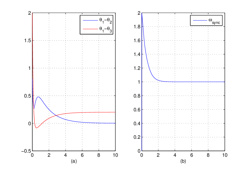
|θ1−θ2θ1−θ3|=|BT​Vθ​z|≤|BT​Vθ|​|z|≤|BT​Vθ|[∗∗𝐛z]=[0.23310.2023].\displaystyle\left|\begin{smallmatrix}\theta_{1}-\theta_{2}\\ \theta_{1}-\theta_{3}\end{smallmatrix}\right|=|B^{T}V_{\theta}z|\leq|B^{T}V_{\theta}||z|\leq|B^{T}V_{\theta}|\left[\begin{smallmatrix}*\\ *\\ \mathbf{b}_{z}\end{smallmatrix}\right]=\left[\begin{smallmatrix}0.2331\\ 0.2023\end{smallmatrix}\right].

where the ∗* entries are irrelevant since the first two columns of BT​VθB^{T}V_{\theta} are zero. The above bounds on the phase differences is validated as can be seen in Fig. 1(a).

The next variable derived from this simulation is the average frequency error as in (3). Corollary III.5 proves that this frequency converges to the steady state frequency ωs​y​n​cs​s{\omega_{sync}}_{ss} as in (34). It is also notable that this steady state average frequency static error is reliant on ϵ\epsilon, that is, by decreasing ϵ\epsilon we obtain a smaller ωs​y​n​cs​s{\omega_{sync}}_{ss}. For ϵ=1\epsilon=1 and ϵ=0.1\epsilon=0.1 the obtained values are

ϵ=1⟶ωs​y​n​cs​s=1,ϵ=0.1⟶ωs​y​n​cs​s=0.1818.\displaystyle\epsilon=1\longrightarrow{\omega_{sync}}_{ss}=1,\quad\epsilon=0.1\longrightarrow{\omega_{sync}}_{ss}=0.1818.

The convergency of ωs​y​n​c\omega_{sync} to ωs​y​n​cs​s{\omega_{sync}}_{ss} for ϵ=1\epsilon=1 is depicted in Fig. 1(b).

Refer to caption
Fig. 1: (a) Line phases, (b) convergence of ωs​y​n​c\omega_{sync} to ωs​y​n​cs​s{\omega_{sync}}_{ss}

V Conclusions

We have analysed theoretical properties of inverter-based microgrids controlled via primary and secondary loops. We have shown that frequency regulation is ensured without the need for time separation, and that ultimate boundedness of the trajectories starting inside a region of the state space is guaranteed under a condition on the inverters power injection errors. The trajectory ultimate bound can be computed by simple iterations of a nonlinear mapping and provides a certificate of the overall performance of the controlled microgrid. Future work includes the derivation of design procedures based on the provided analysis, the extension of the results to more general controller parameters and structures as well as relaxing some of the modelling assumptions.

References

  • [1] N. Ainsworth and S. Grijalva. A structure-preserving model and sufficient condition for frequency synchronization of lossless droop inverter-based AC networks. IEEE Trans. on Power Syst., 28(4):4310–4319, 2013.
  • [2] N. Ainsworth and S. Grijalva. Design and quasi-equilibrium analysis of a distributed frequency-restoration controller for inverter-based microgrids. In North American Power Symposium, pages 1–6, 2013.
  • [3] M. Andreasson, H. Sandberg, D.V. Dimarogonas, and K.H. Johansson. Distributed integral action: Stability analysis and frequency control of power systems. In IEEE Conf. on Dec. and Control, Hawai, 2012.
  • [4] A. Bidram and A. Davoudi. Hierarchical structure of microgrids control system. IEEE Transactions on Smart Grid, 3(4):1963–1976, 2012.
  • [5] M.C. Chandorkar, D.M. Divan, and R. Adapa. Control of parallel connected inverters in standalone AC supply systems. IEEE Transactions on Industry Applications, 29(1):136–143, 1993.
  • [6] F. Dörfler, J.W. Simpson-Porco, and F. Bullo.
  • [7] J.M. Guerrero, J.C. Vasquez, J. Matas, L.G. de Vicuña, and M. Castilla. Hierarchical Control of Droop-Controlled AC and DC Microgrids–A General Approach Toward Standardization. IEEE Transactions on Industrial Electronics, 58(1):158–172, 2011.
  • [8] H. Haimovich and M.M. Seron. Bounds and invariant sets for a class of switching systems with delayed-state-dependent perturbations, 2012. Available at http://arxiv.org/abs/1202.0455.
  • [9] H. Haimovich and M.M. Seron. Bounds and invariant sets for a class of switching systems with delayed-state-dependent perturbations. Automatica, 49(3):748–754, 2013.
  • [10] H. Khalil. Nonlinear Systems. Prentice-Hall, NJ, 3rd edition, 2002.
  • [11] R.H. Lasseter. Microgrids. In IEEE Power Engineering Society Winter Meeting, volume 1, pages 146–149, 2001. Panel: Role of Distributed Generation in Reinforcing the Critical Electric Power.
  • [12] J.A. Peças Lopes, C.L. Moreira, and A.G. Madureira. Defining control strategies for MicroGrids islanded operation. IEEE Transactions on Power Systems, 21(2):916–924, 2006.
  • [13] F.Z. Peng, Y.W. Li, and L.M. Tolbert. Control and protection of power electronics interfaced distributed generation systems in a customer-driven microgrid. In IEEE Power & Energy Society General Meeting, PES’09, 2009.
  • [14] J. Schiffer, A. Anta, T.D. Truong, J. Raisch, and T. Sezi. On power sharing and stability in autonomous inverter-based microgrids. In IEEE Conf. on Decision and Control, Maui, Hawaii, USA, December 2012.
  • [15] Q. Shafiee, J.C. Vasquez, and J.M. Guerrero. Distributed secondary control for islanded MicroGrids—a networked control systems approach. In Annual Conf. IEEE Industrial Electronics Society, 2012.
  • [16] J.W. Simpson-Porco, F. Dörfler, and F. Bullo. Synchronization and power sharing for droop-controlled inverters in islanded microgrids. Automatica, 49(9):2603–2611, 2013.
  • [17] T.S. Ustun, C. Ozansoy, and A. Zayegh. Recent developments in microgrids and example cases around the world. A review. Renewable and Sustainable Energy Reviews, 15(8):4030–4041, October 2011.
  • [18] A.I. Zecevic, G.Neskovic, and D.A. Siljak. Robust decentralized exciter control with linear feedback. IEEE Transactions on Power Systems, 19(2):1096–1103, 2004.
  • [19] Q.-C. Zhong and T. Hornik. Control of Power Inverters in Renewable Energy and Smart Grid Integration. John Wiley & Sons, 2013.