跳到论文正文
W Papers独立论文阅读器 arXiv:1409.4394 论文正文 计算阅读时间 · 0%
引用这篇论文根据当前论文元数据生成,正式投稿前建议核对。


License: arXiv.org perpetual non-exclusive license
arXiv:1409.4394v2 [physics.gen-ph] 12 Jan 2015

The Dark Energy Star and Stability analysis

Piyali Bhar Email: piyalibhar90@gmail.com Affiliation:  Department of Mathematics, Jadavpur University, Kolkata 700 032, West Bengal, India    Farook Rahaman Email: rahaman@iucaa.ernet.in Affiliation:  Department of Mathematics, Jadavpur University, Kolkata 700 032, West Bengal, India
Abstract

Abstract: We have proposed a new model of dark energy star consisting of five zones namely, solid core of constant energy density, the thin shell between core and interior, an inhomogeneous interior region with anisotropic pressures, thin shell and the exterior vacuum region. We have discussed various physical properties. The model satisfies all the physical requirements. The stability condition under small linear perturbation has also been discussed.

I Introduction

The study of dark energy star has become a subject of interest due to the fact that expansion of the universe is accelerating which was suggested by High-z supernova Search Team in 19981998 by observing type 1​a1a supernova. Dark energy is the most acceptable hypothesis to explain this accelerating expansion of the universe. According to the work done of Plank mission team and based on the standard model of cosmology the total mass energy of the universe contains 4.94.9 percent ordinary matter, 26.826.8 percent dark matter and 68.368.3 percent dark energy. Dark matter is attractive in nature which can not seen by a telescope and it does not absorbs or emits light or any gravitational waves. But its existence has been proved by gravitational effects on visible matter and gravitational lensing of background radiation. On the other hand the dark energy needs to have a strong negative pressure in order to explain the rate of accelerating expansion of the universe.

To construct a model of a relativistic star we generally assume that the underlying fluid distribution is homogeneous and isotropic. But it is proved by advance researches that the highly compact astrophysical objects like X-ray pulsar, Her-x-1, X-ray buster 4U 1820-30, millisecond pulsar SAXJ1804.4-3658 etc. whose density of core is expected to be beyond the nuclear density (∼1015​g​m/c​c)(\sim 10^{15}gm/cc) shows the anisotropy. Anisotropy may occurs in the existence of solid core, in presence of type P superfluid, phase transition, rotation, magnetic field, mixture of two fluid, existence of external field etc. In case of anisotropy distribution the pressure inside the fluid sphere is not homogeneous in nature, it can be decomposed into two parts radial pressure prp_{r} and the transverse pressure ptp_{t}. So obviously pr≠ptp_{r}\neq p_{t}. Where ptp_{t} is in the orthogonal direction to prp_{r}. Δ=pt−pr\Delta=p_{t}-p_{r} is defined as the anisotropic factor whereas Δr\frac{\Delta}{r} is defined as anisotropic force which is repulsive in nature if pt>prp_{t}>p_{r} and attractive if pt<prp_{t}<p_{r}.

In this paper,we are going to model of a anisotropic dark energy star characterized by the parameter ω=prρ\omega=\frac{p_{r}}{\rho}, where prp_{r} and ρ\rho are respectively the radial pressure and energy density. For accelerating expansion the dark energy parameter ω<−13\omega<-\frac{1}{3} is required. −1<ω<−13-1<\omega<-\frac{1}{3} is referred to as quintessence. The region where ω<−1\omega<-1 is named as phantom regime which has a peculiar property namely infinitely increasing energy density. ω=−1\omega=-1 corresponds to Einstein cosmological constant and this value is called cosmological constant barrier or phantom divide.

A two dimensional Brans-Dicke star model with exotic matter and dark energy was studied in [1]. In that paper, the author has taken the matter state equation as p=γ​ρp=\gamma\rho, where γ\gamma is the state parameter of exotic matter which satisfies −14<γ<0-\frac{1}{4}<\gamma<0 and has shown that the mass of the star decrease if γ\gamma decrease. Anisotropic dark energy star has been discussed in [2]. Star model with dark energy has been proposed in [3]. In this paper the authors have proposed a model of dark energy star consisting of four region and by analyzing the model they conclude that for static solution at least one of the regions must be constituted by dark energy. Anisotropic dark energy star was studied by Ghezzi et al [4]. In this paper the authors have assumed variable dark energy which suffers a phase transition at a critical density and the anisotropy. The anisotropy is concentrated on a thin shell where the phase transition takes place, while the rest of the star remains isotropic. The solutions shows several features similar to the gravastar model. Lobo[5] has given a model of stable dark energy star by assuming two spatial type of mass function one is of constant energy density and the other mass function is Tolman-Whitker mass. All the features of the dark energy star has been discussed and the system is stable under small linear perturbation. The van der Waals quintessence stars have been studied in [6]. In that work, the construction of inhomogeneous compact spheres supported by a van der Waals equation of state is explored. van der Waals gravastar, van der Waals wormhole have also been discussed. Variable Equation of State for Generalised Dark Energy Model has been studied in [7]. Yadav et al.have given a dark energy models with variable equation of state parameter in [8]. Some other works on dark energy star are in [15, 16, 17, 18, 19, 20, 21, 22].

The plan of the paper is as follows: In section II basic field equations have been given. The model of dark energy star,exterior spacetime and junction condition, TOV equation,Energy condition, Mass-radius relation have been respectively discussed in section III-VII. The stability analysis under small radial perturbation has been studied in section VIII. Finally in section IX we have provided a short discussion and made some concluding remarks.

II Basic Field Equations

A static and spherically symmetry spacetime in curvature coordinates is given by the following metric

ds2=−exp[−2∫r∞g(r~)dr~]dt2+d​r21−2​mrds^{2}=-exp\left[{-2\int_{r}^{\infty}g(\tilde{r})d\tilde{r}}\right]dt^{2}+\frac{dr^{2}}{1-\frac{2m}{r}}
+r2​(d​θ2+sin2⁡θ​d​ϕ2),~~~~~~~~~~~~~~~~~~~~~~+r^{2}(d\theta^{2}+\sin^{2}\theta d\phi^{2}), (1)

where g⁡(r)g(r) and m⁡(r)m(r) are arbitrary functions of the radial parameters r. The function m⁡(r)m(r) is the quasi local mass and is denoted as the mass function.The factor g⁡(r)g(r) is termed as the ’gravity profile’ which is used to measure the acceleration due to gravity by the relationship 𝒜=1−2​mr​g​(r)\mathcal{A}=\sqrt{1-\frac{2m}{r}}g(r). For inward gravitational attraction g⁡(r)>0g(r)>0 and g⁡(r)<0g(r)<0 for outward gravitational repulsion. One can note that Φ(r)=−∫r∞g(r)dr\Phi(r)=-\int_{r}^{\infty}g(r)dr, here Φ⁡(r)\Phi(r) is denoted as the redshift function.

The stress energy momentum tensor is given by the equation

Tμ​ν=(ρ+pt)​Uμ​Uμ+pt​gμ​ν+(pr−pt)​χμ​χνT_{\mu\nu}=(\rho+p_{t})U_{\mu}U_{\mu}+p_{t}g_{\mu\nu}+(p_{r}-p_{t})\chi_{\mu}\chi_{\nu} (2)

where UμU^{\mu} is the vector 44-velocity,χμ\chi^{\mu} is the spacelike vector. ρ⁡(r)\rho(r) is the energy density and prp_{r} is the radial pressure measured in the direction of the spacelike vector. ptp_{t} is the transverse pressure in the orthogonal direction to prp_{r} and Δ=pt−pr\Delta=p_{t}-p_{r} is called the anisotropic factor.

Using the Einstein field equations Gμ​ν=8​π​Tμ​νG_{\mu\nu}=8\pi T_{\mu\nu} we get the following relationship,

m′=4​π​r2​ρm^{\prime}=4\pi r^{2}\rho (3)
g=m+4​π​r3​prr⁡(r−2​m)g=\frac{m+4\pi r^{3}p_{r}}{r(r-2m)} (4)
pr′=−(ρ+pr)​(m+4​π​r3​pr)r⁡(r−2​m)+2r​(pt−pr)p_{r}^{\prime}=-\frac{(\rho+p_{r})(m+4\pi r^{3}p_{r})}{r(r-2m)}+\frac{2}{r}(p_{t}-p_{r}) (5)

where Gμ​νG_{\mu\nu} is the Einstein tensor and ’prime’ denotes the derivative with respect to radial coordinate rr.
The dark energy equation of state is given by the following equation

pr=ω​ρp_{r}=\omega\rho (6)

where ω<0\omega<0 is the equation of state parameter.

Now one can note that we have five unknown functions namely ρ,pr,pt,m⁡(r),g⁡(r)\rho,p_{r},p_{t},m(r),g(r) and four equations[(3)-(6)]. To solve the set of equations let us assume a particular choice of the energy density ρ\rho. This particular choice of ρ\rho was chosen earlier by Dev and Gleiser [9] to discuss anisotropic star model. Rahaman et al.have also used this density function in[10]. Using this particular choice of energy density we will find out the other parameters in explicit form.

III Model of the dark energy Star

Let us choose the energy density of the star as

ρ=18​π​(ar2+3​b)\rho=\frac{1}{8\pi}\left(\frac{a}{r^{2}}+3b\right) (7)

where both aa and bb are constants, e.g a=37a=\frac{3}{7} and b=0b=0 corresponds to relativistic Fermi gas which can be seen in the ultradense cores of a neutron star [11] and for a=37,b≠0a=\frac{3}{7},b\neq 0 we get relativistic fermi gas core in a constant density background.
Using (7)(7) into (3)(3) we obtain the expression of the mass function as,

m=12​r​(a+b​r2)m=\frac{1}{2}r(a+br^{2}) (8)

Solving equation (4)−(6)(4)-(6) we get,

g⁡(r)=a⁡(1+ω)+b​r2​(1+3​ω)2​r​(1−a−b​r2),g(r)=\frac{a(1+\omega)+br^{2}(1+3\omega)}{2r(1-a-br^{2})}, (9)

From Buchdahl limit, 2​m​(r)r<1\frac{2m(r)}{r}<1 one can see from equation (8) as 1−a−b​r2>01-a-br^{2}>0. This provides a constraint on the parameters a,ba,~b and radius r as

r2<1−ab(9.1)r^{2}<\frac{1-a}{b}~~~~~~~~~~~~~~~~~~~~~~~~~~~~~~~~~~~~~~~~~~~~~~~~~~~~~~~~~~(9.1)

This yields the restriction on a,ba,~b as

a<1​a​n​d​b>0.a<1~and~b>0.

We have chosen a=0.5a=0.5 and b=0.00b=0.001 motivated by the choice of Dev and Glaiser [9]. They chose a=3/7a=3/7 and b=0b=0 to describe their model. Our chosen values of aa and bb are very close to their choice. Now using those values for aa and bb from equation (9.1), we get r2<500r^{2}<500 i.e r<22.36r<22.36. Now, g⁡(r)>0g(r)>0 gives,

ω>−a+b​r2a+3​b​r2(9.2)\omega>-\frac{a+br^{2}}{a+3br^{2}}~~~~~~~~~~~~~~~~~~~~~~~~~~~~~~~~~~~~~~~~~~~~~~~~~~~~~~~~~~(9.2)

For large r i.e. in the maximum limit, we get by using (9.1) in (9.2) as

ω>−13−2​a\omega>-\frac{1}{3-2a}

For small r, from (9.2) we have ω>−1\omega>-1.
Therefore,

ω>m​a​x​(−1,−13−2​a)(9.3)\omega>max\left(-1,-\frac{1}{3-2a}\right)~~~~~~~~~~~~~~~~~~~~~~~~~~~~~~~~~~~~~~~~~~~~~~(9.3)

For the above choice, a=0.5a=0.5, m​a​x​(−1,−13−2​a)=−0.5max\left(-1,-\frac{1}{3-2a}\right)=-0.5 i.e. ω>−0.5\omega>-0.5.

Again for g⁡(r)<0g(r)<0, we have

ω<−a+b​r2a+3​b​r2(9.4)\omega<-\frac{a+br^{2}}{a+3br^{2}}~~~~~~~~~~~~~~~~~~~~~~~~~~~~~~~~~~~~~~~~~~~~~~~~~~~~~~~~~(9.4)

For small r, equation (9.4) yields
ω<−1\omega<-1 and for large r i.e. in the maximum limit,

ω<−13−2​a\omega<-\frac{1}{3-2a}

Thus,

ω<m​i​n​(−1,−13−2​a)(9.5)\omega<min\left(-1,-\frac{1}{3-2a}\right)~~~~~~~~~~~~~~~~~~~~~~~~~~~~~~~~~~~~~~~~~~~(9.5)

For our choice of aa, we get ω<−1\omega<-1. So, we have to choose ω\omega either ω>−0.5\omega>-0.5 or ω<−1\omega<-1 for plot.

The profiles of g(r) have been plotted in f​i​g​1fig~1 and f​i​g​2fig~2 for −0.45≤ω≤−0.1-0.45\leq\omega\leq-0.1 and ω<−1\omega<-1 respectively.
From the fig. 1 we see that g⁡(r)>0g(r)>0 when −0.45≤ω≤−0.1-0.45\leq\omega\leq-0.1 and fig. 2 shows that for ω<−1\omega<-1, g⁡(r)<0g(r)<0 for above choice of aa and bb.

Refer to caption
Figure 1: “gravity profile”, g⁡(r)g(r),  has been plotted against rr when −0.45≤ω≤−0.1-0.45\leq\omega\leq-0.1

The radial and transverse pressure can be obtained as,

pr=ω8​π​(ar2+3​b)p_{r}=\frac{\omega}{8\pi}\left(\frac{a}{r^{2}}+3b\right) (10)
pt=(1+ω)​(a+3​b​r2)32​π​r2​(1−a−b​r2)​[a⁡(1+ω)+b​r2​(1+3​ω)]+3​b​ω8​πp_{t}=\frac{(1+\omega)(a+3br^{2})}{32\pi r^{2}(1-a-br^{2})}\left[a(1+\omega)+br^{2}(1+3\omega)\right]+\frac{3b\omega}{8\pi} (11)

The matter density, radial and transverse pressures have been depicted in f​i​g​3.fig~3.
The anisotropy factor Δ\Delta is given by,

Δ=(1+ω)​(a+3​b​r2)32​π​r2​(1−a−b​r2)​[a⁡(1+ω)+b​r2​(1+3​ω)]−ω​a8​π​r2,\Delta=\frac{(1+\omega)(a+3br^{2})}{32\pi r^{2}(1-a-br^{2})}\left[a(1+\omega)+br^{2}(1+3\omega)\right]-\frac{\omega a}{8\pi r^{2}}, (12)

which has been shown in f​i​g​.4fig.4 and f​i​g​.5fig.5 respectively for −0.45≤ω≤−0.1-0.45\leq\omega\leq-0.1 and ω<−1\omega<-1. Now Δr\frac{\Delta}{r} re presents a force due to the pressure anisotropy. The force will be repulsive in nature i.e. in the outward direction if pt>prp_{t}>p_{r} and attractive if pt<prp_{t}<p_{r} or alternatively Δ<0\Delta<0. For our stellar model configuration (see fig.4 and fig.5) Δ>0\Delta>0 for both the cases when −0.5<ω<−0.1-0.5<\omega<-0.1 and for phantom regime i.e. for ω<−1\omega<-1.

Refer to caption
Figure 2: “gravity profile”, g⁡(r)g(r), has been plotted against rr when ω≤−1\omega\leq-1, a=0.45a=0.45 and b=0.001b=0.001.
Refer to caption
Figure 3: Matter density ρ\rho,radial pressure prp_{r} and transverse pressure ptp_{t} of the dark energy model has been plotted against rr
Refer to caption
Figure 4: The anisotropy parameter Δ=pt−pr\Delta=p_{t}-p_{r} has been shown against rr for −0.45≤ω≤−0.1-0.45\leq\omega\leq-0.1.
Refer to caption
Figure 5: The anisotropy parameter Δ=pt−pr\Delta=p_{t}-p_{r} has been shown against rr for ω<−1\omega<-1

Now, one can notice that there is a problem in the model such as the divergence of the physical quantities (energy density and pressures) in the origin. Now to overcome this problem in order to model a star, we propose that the star contains a core up to radius r1r_{1}.

III.1 Core Solution

To avoid this central singularity we cut the spacetime (1) around its origin and placed an anisotropy fluid of constant density ρ0\rho_{0} (say).
Now, to find the core solution, we assume the radial equation of state as,

pr=k​ρ0,k<0p_{r}=k\rho_{0},~~~~k<0 (13)

Here, the mass function becomes,

m⁡(r)=B​r3m(r)=Br^{3} (14)

where B=4​π​ρ03B=\frac{4\pi\rho_{0}}{3}.

Using this expression of m⁡(r)m(r) from equation (4) and using equation (14) we get,

g⁡(r)=B​r​(1+3​k)1−2​B​r2g(r)=\frac{Br(1+3k)}{1-2Br^{2}} (15)

Therefore the spacetime metric of the core is given by

d​s2=(1−2​B​r2)−1+3​k2​d​t2+d​r21−2​B​r2+r2​(d​θ2+sin2⁡θ​d​ϕ2)ds^{2}=(1-2Br^{2})^{-\frac{1+3k}{2}}dt^{2}+\frac{dr^{2}}{1-2Br^{2}}+r^{2}(d\theta^{2}+\sin^{2}\theta d\phi^{2}) (16)

The transverse pressure can be obtained as

pt=k​ρ0​[1+(1+k)​(1+3​k)​B​r22​k​(1−2​B​r2)]p_{t}=k\rho_{0}\left[1+\frac{(1+k)(1+3k)Br^{2}}{2k(1-2Br^{2})}\right] (17)

and the anisotropic factor Δ\Delta can be obtained as,

Δ=38​π​(1+k)​(1+3​k)​B2​r21−2​B​r2\Delta=\frac{3}{8\pi}(1+k)(1+3k)\frac{B^{2}r^{2}}{1-2Br^{2}} (18)

From the expression of Δ\Delta it is clear that Δ>0\Delta>0 if k<−1k<-1 and Δ<0\Delta<0 if −1<k<−13-1<k<-\frac{1}{3}. At the center of the star Δ=0\Delta=0 which is expected for a physically reasonable solution. It can also be noted that for k=−1k=-1 and k=−13k=-\frac{1}{3} the anisotropic pressure of the core reduces to isotropic pressure.

IV Energy Conditions

Our particular model of dark energy star consists of five regions:

  1. 1.

    Solid core of constant matter density

  2. 2.

    Thin shell between core and Interior

  3. 3.

    Interior

  4. 4.

    Thin shell between interior and exterior spacetime

  5. 5.

    Exterior Schwarzschild spacetime

To check whether our model satisfies all the energy conditions, we have to verify the energy conditions in first four regions described earlier.

At first check all the energy conditions, for regions 1 and 3 and later we will discuss the region 2. We will consider the following inequalities:

(i)​N​E​C:ρ+pr≥0(i)~NEC:\rho+p_{r}\geq 0 (19)
(i​i)​W​E​C:ρ+pr≥0,ρ≥0(ii)~WEC:\rho+p_{r}\geq 0,~~\rho\geq 0 (20)
(i​i​i)​S​E​C:ρ+pr≥0,ρ+pr+2​pt≥0(iii)~SEC:\rho+p_{r}\geq 0,~~~\rho+p_{r}+2p_{t}\geq 0 (21)
(i​v)​D​E​C:ρ>|pr|,ρ>|pt|(iv)~DEC:\rho>\left|p_{r}\right|,~~~\rho>\left|p_{t}\right| (22)

The fig:6 indicates that for our model, all the energy conditions are satisfied in the interior region. The fig:7, however, shows the SEC is violated within the core.

Refer to caption
Figure 6: The energy conditions in the interior has been plotted against rr
Refer to caption
Figure 7: The energy condition of within the core has been plotted against rr.

V Exterior Spacetime and Junction Condition

In this section we match our interior spacetime to the exterior schwarzschild vacuum solution along the junction surface with the junction radius R′′{}^{\prime}R^{\prime}.The exterior spacetime is given by the metric

d​s2=−(1−2​Mr)​d​t2+d​r21−2​Mr+r2​(d​θ2+sin2⁡θ​d​ϕ2)ds^{2}=-\left(1-\frac{2M}{r}\right)dt^{2}+\frac{dr^{2}}{1-\frac{2M}{r}}+r^{2}(d\theta^{2}+\sin^{2}\theta d\phi^{2}) (23)

Here,event horizon lies at r=2​Mr=2M.So obviously R>2​MR>2M.

Previously, we have matched our interior spacetime to the exterior Schwarzschild at the boundary r=Rr=R. Obviously the metric coefficients are continuous at r=Rr=R, but it does not ensure that their derivatives are also continuous at the junction surface. In other words the affine connections may be discontinuous there. To take care of this let us use the Darmois-Israel[12, 13] formation to determine the surface stresses at the junction boundary. The intrinsic surface stress energy tensor Si​jS_{ij} is given by Lancozs equations in the following form

Sji=−18​π​(κji−δji​κkk)S^{i}_{j}=-\frac{1}{8\pi}(\kappa^{i}_{j}-\delta^{i}_{j}\kappa^{k}_{k}) (24)

The discontinuity in the second fundamental form is given by,

Ki​j=Ki​j+−Ki​j−K_{ij}=K_{ij}^{+}-K_{ij}^{-} (25)

where the second fundamental form is given by,

Ki​j±=−nν±​[∂2Xν∂ξ1​∂ξj+Γα​βν​∂Xα∂ξi​∂Xβ∂ξj]|S,K_{ij}^{\pm}=-n_{\nu}^{\pm}\left[\frac{\partial^{2}X_{\nu}}{\partial\xi^{1}\partial\xi^{j}}+\Gamma_{\alpha\beta}^{\nu}\frac{\partial X^{\alpha}}{\partial\xi^{i}}\frac{\partial X^{\beta}}{\partial\xi^{j}}\right]|_{S}, (26)

where nν±n_{\nu}^{\pm} are the unit normal vector defined by,

nν±=±|gα​β​∂f∂Xα​∂f∂Xβ|−12​∂f∂Xν,n_{\nu}^{\pm}=\pm\left|g^{\alpha\beta}\frac{\partial f}{\partial X^{\alpha}}\frac{\partial f}{\partial X^{\beta}}\right|^{-\frac{1}{2}}\frac{\partial f}{\partial X^{\nu}}, (27)

with nν​nν=1n^{\nu}n_{\nu}=1. Here ξi\xi^{i} is the intrinsic coordinate on the shell.++and−- corresponds to exterior i.e., Schwarzschild spacetime and interior(our) spacetime respectively. The model of our dark energy star is consisting with five zones namely, core, the thin shell between core and interior, an inhomogeneous interior region with anisotropic pressures, thin shell and the exterior vacuum region.

Considering the spherical symmetry of the spacetime surface stress energy tensor can be written as Sji=d​i​a​g​(−σ,𝒫,𝒫)S^{i}_{j}=diag(-\sigma,\mathcal{P},\mathcal{P}), where σ\sigma and 𝒫\mathcal{P} are the surface energy density and surface pressure respectively.

Kττ+=MR2+R¨1−2​MR+R˙2K_{\tau}^{\tau+}=\frac{\frac{M}{R^{2}}+\ddot{R}}{\sqrt{1-\frac{2M}{R}+\dot{R}^{2}}} (28)
Kττ−=(1+ω)​a+b​R2​(1+3​ω)2​R+R¨−(1+ω)​R˙2​(a+3​b​R2)2​(R−R​a−b​R3)1−a−b​R2+R˙2K_{\tau}^{\tau-}=\frac{\frac{(1+\omega)a+bR^{2}(1+3\omega)}{2R}+\ddot{R}-\frac{(1+\omega)\dot{R}^{2}(a+3bR^{2})}{2(R-Ra-bR^{3})}}{\sqrt{1-a-bR^{2}+\dot{R}^{2}}} (29)
Kθθ+=1R​1−2​MR+R˙2K_{\theta}^{\theta+}=\frac{1}{R}\sqrt{1-\frac{2M}{R}+\dot{R}^{2}} (30)
Kθθ−=1R​1−a−b​R2+R˙2K_{\theta}^{\theta-}=\frac{1}{R}\sqrt{1-a-bR^{2}+\dot{R}^{2}} (31)

The expressions of σ\sigma and 𝒫\mathcal{P} are given by,

σ=−14​π​R​[1−2​MR+R˙2−1−(a+b​R2)+R˙2]\sigma=-\frac{1}{4\pi R}\left[\sqrt{1-\frac{2M}{R}+\dot{R}^{2}}-\sqrt{1-(a+bR^{2})+\dot{R}^{2}}\right] (32)
𝒫=18​π​R​[1−MR+R˙2+R​R¨1−2​MR+R˙2+1+R​g​(R)​(1−a−b​R2+R˙2)+R​R¨+b​R21−a−b​R2​R˙21−a−b​R2+R˙2]\mathcal{P}=\frac{1}{8\pi R}\left[\frac{1-\frac{M}{R}+\dot{R}^{2}+R\ddot{R}}{\sqrt{1-\frac{2M}{R}+\dot{R}^{2}}}+\frac{1+Rg(R)(1-a-bR^{2}+\dot{R}^{2})+R\ddot{R}+\frac{bR^{2}}{1-a-bR^{2}}\dot{R}^{2}}{\sqrt{1-a-bR^{2}+\dot{R}^{2}}}\right] (33)

Using conservation identity Sj,ii=−[σ˙+2​R˙R​(𝒫+σ)]S_{j,i}^{i}=-[\dot{\sigma}+2\frac{\dot{R}}{R}(\mathcal{P}+\sigma)], one can obtain

σ′=−2R​(𝒫+σ)+Ξ\sigma^{\prime}=-\frac{2}{R}(\mathcal{P}+\sigma)+\Xi (34)

where Ξ\Xi is given by,

Ξ=−14​π​R​m−m′​RR−2​m​1−a−b​R2+R˙2\Xi=-\frac{1}{4\pi R}\frac{m-m^{\prime}R}{R-2m}\sqrt{1-a-bR^{2}+\dot{R}^{2}} (35)

The surface mass of the thin shell is given by

ms=4​π​R2​σm_{s}=4\pi R^{2}\sigma (36)

Using the expression of σ\sigma given in equation (22)(22) (considering the static case) we get,

ms=R⁡[1−(a+b​R2)−1−2​MR]m_{s}=R\left[\sqrt{1-(a+bR^{2})}-\sqrt{1-\frac{2M}{R}}\right] (37)

After some little manipulation of equation (27)(27) the total mass of the dark energy star can be obtained as,

M=12​R​(a+b​R2)−ms22​R+ms​1−(a+b​R2)M=\frac{1}{2}R(a+bR^{2})-\frac{m_{s}^{2}}{2R}+m_{s}\sqrt{1-(a+bR^{2})} (38)

From equation (27)(27) one can obtain

(ms2​R)′′=Υ−4​π​σ′​η\left(\frac{m_{s}}{2R}\right)^{\prime\prime}=\Upsilon-4\pi\sigma^{\prime}\eta (39)

(for details calculation see the appendix) where,

η=𝒫′σ′,Υ=4​πR​(σ+𝒫)+2​π​R​Ξ′\eta=\frac{\mathcal{P^{\prime}}}{\sigma^{\prime}},~~~~~~~~\Upsilon=\frac{4\pi}{R}(\sigma+\mathcal{P})+2\pi R\Xi^{\prime} (40)

where the ’prime’ denotes derivative with respect to ’R’.

We will use the parameter η\eta to discuss the stability analysis of the system. This η\sqrt{\eta} is generally interpreted as the velocity of the sound. So, for the physical acceptability one must have 0<η≤10<\eta\leq 1. The profile of η\eta has been shown in f​i​g​.8fig.8 and f​i​g​.9fig.9.

Next we will discuss about the evolution identity given by,

[Tμ​ν​nμ​nν]−+=K¯ji​Sij\left[T_{\mu\nu}n^{\mu}n^{\nu}\right]_{-}^{+}=\bar{K}_{j}^{i}S_{i}^{j} (41)

where K¯ji=12​(Kji++Kji−)\bar{K}_{j}^{i}=\frac{1}{2}\left(K_{j}^{i+}+K_{j}^{i-}\right) From equation (31)(31) using the equation (18)−(21)(18)-(21) one can obtain

pr+(ρ+pr)​R˙21−a−b​R2=−12​R​(1−2​MR+R˙2+1−a−b​R2+R˙2)​𝒫p_{r}+\frac{(\rho+p_{r})\dot{R}^{2}}{1-a-bR^{2}}=-\frac{1}{2R}\left(\sqrt{1-\frac{2M}{R}+\dot{R}^{2}}+\sqrt{1-a-bR^{2}+\dot{R}^{2}}\right)\mathcal{P}
+12​(MR2+R¨1−2​MR+R˙2+(1+ω)​a+b​R2​(1+3​ω)2​R+R¨−(1+ω)​R˙2​(a+3​b​R2)2​(R−R​a−b​R3)1−a−b​R2+R˙2)​σ+\frac{1}{2}\left(\frac{\frac{M}{R^{2}}+\ddot{R}}{\sqrt{1-\frac{2M}{R}+\dot{R}^{2}}}+\frac{\frac{(1+\omega)a+bR^{2}(1+3\omega)}{2R}+\ddot{R}-\frac{(1+\omega)\dot{R}^{2}(a+3bR^{2})}{2(R-Ra-bR^{3})}}{\sqrt{1-a-bR^{2}+\dot{R}^{2}}}\right)\sigma (42)

Considering static solution at R=R0R=R_{0} with R˙=R¨=0\dot{R}=\ddot{R}=0, we get,

pr=−12​R0​(1−2​MR0+1−a−b​R02)​𝒫+12​(MR021−2​MR0+(1+ω)​a+b​R02​(1+3​ω)2​R01−a−b​R02)​σp_{r}=-\frac{1}{2R_{0}}\left(\sqrt{1-\frac{2M}{R_{0}}}+\sqrt{1-a-bR_{0}^{2}}\right)\mathcal{P}+\frac{1}{2}\left(\frac{\frac{M}{R_{0}^{2}}}{\sqrt{1-\frac{2M}{R_{0}}}}+\frac{\frac{(1+\omega)a+bR_{0}^{2}(1+3\omega)}{2R_{0}}}{\sqrt{1-a-bR_{0}^{2}}}\right)\sigma (43)

Here, σ<0\sigma<0, therefore, pr<0,p_{r}<0, i.e. tension is in radial direction. Hence a positive tangential surface pressure P>0P>0 is required to keep the shell stable i.e. to hold the shell against collapsing.

Refer to caption
Figure 8: The velocity of the sound for different values of mass MM has been plotted against rr when the dark energy parameter ω\omega is fixed
Refer to caption
Figure 9: The velocity of the sound for different values of energy parameter ω\omega has been plotted against rr when the mass of the dark energy star MM is fixed

V.1 Junction conditions between core and interior solution

Since core radius is r1r_{1}, therefore, we match the core solution with interior solution at the junction surface with junction radius r1r_{1}.

The core extrinsic curvature is given by,

Kτ​τ−=−B​r1​(1+3​k)​(1−2​B​r12)−12K_{\tau\tau}^{-}=-Br_{1}(1+3k)(1-2Br_{1}^{2})^{-\frac{1}{2}}
Kθ​θ−=r1​(1−2​B​r12)12K_{\theta\theta}^{-}=r_{1}(1-2Br_{1}^{2})^{\frac{1}{2}}

Therefore the surface energy density and surface pressure can be obtained as,

σ=−14​π​r1​[1−a−b​r12−1−2​B​r12]\sigma=-\frac{1}{4\pi r_{1}}\left[\sqrt{1-a-br_{1}^{2}}-\sqrt{1-2Br_{1}^{2}}\right] (44)
𝒫=18​π​r1​[1+r1​g​(r1)​(1−a−b​r12)1−a−b​r12−1+(1+3​k)​B​r121−2​B​r12]\mathcal{P}=\frac{1}{8\pi r_{1}}\left[\frac{1+r_{1}g(r_{1})(1-a-br_{1}^{2})}{\sqrt{1-a-br_{1}^{2}}}-\frac{1+(1+3k)Br_{1}^{2}}{\sqrt{1-2Br_{1}^{2}}}\right] (45)

V.2 Energy conditions for both the thin shells i.e. Interior thin shell between core and interior region and Outer thin shell between the interior region and the Schwarzschild spacetime

According to [25] for a thin shell all the energy conditions namely Null Energy conditions (NEC), Weak Energy Conditions (WEC), Dominant Energy conditions (DEC), Strong Energy Conditions (SEC) will be satisfied if the following inequalities hold.

  1. 1.

    NEC : σ+𝒫≥0\sigma+\mathcal{P}\geq 0

  2. 2.

    WEC : σ≥0\sigma\geq 0 and σ+𝒫≥0\sigma+\mathcal{P}\geq 0

  3. 3.

    SEC : σ+𝒫≥0\sigma+\mathcal{P}\geq 0 and σ+2​𝒫≥0\sigma+2\mathcal{P}\geq 0

  4. 4.

    DEC : σ+𝒫≥0\sigma+\mathcal{P}\geq 0 and σ−𝒫≥0\sigma-\mathcal{P}\geq 0

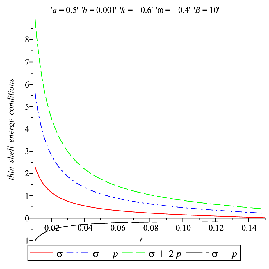
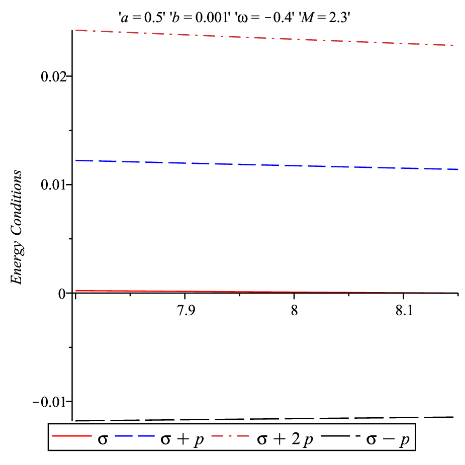
The f​i​g​.10fig.10 and f​i​g​.11fig.11 show all energy conditions except DEC, is violated within both interior and exterior thin shells.
Refer to caption
Figure 10: The energy condition of the thin shell between core and interior region has been plotted against rr.
Refer to caption
Figure 11: The energy condition of the thin shell between interior region and the exterior Schwarzschild spacetime has been plotted against rr.

VI TOV Equation

The generalized Tolman-Oppenheimer-Volkov (TOV) equation is given by the equation [14]

−MG​(ρ+pr)r2​eλ−ν2−d​prd​r+2r​(pt−pr)=0-\frac{M_{G}(\rho+p_{r})}{r^{2}}e^{\frac{\lambda-\nu}{2}}-\frac{dp_{r}}{dr}+\frac{2}{r}(p_{t}-p_{r})=0 (46)

Where MG=MG​(r)M_{G}=M_{G}(r) is the effective gravitational mass inside a sphere of radius rr given by the Tolmam-Whittaker formula which can be derived from the equation

MG​(r)=12​r2​eν−λ2​ν′M_{G}(r)=\frac{1}{2}r^{2}e^{\frac{\nu-\lambda}{2}}\nu^{\prime} (47)

The above equations describes the equilibrium conditions of the fluid sphere subject to gravitational,hydrostatics and anisotropy forces.

Refer to caption
Figure 12: The dark energy star is in static equilibrium under gravitational (Fg)(F_{g}),hydrostatics (Fh)(F_{h}) and anisotropy (Fa)(F_{a}) forces.

The equation (34)(34) can be modified in the form

Fg+Fh+Fa=0F_{g}+F_{h}+F_{a}=0 (48)

where

Fg=−ν′2​(ρ+pr)F_{g}=-\frac{\nu^{\prime}}{2}(\rho+p_{r}) (49)
Fh=−d​prd​rF_{h}=-\frac{dp_{r}}{dr} (50)
Fa=2r​(pt−pr)F_{a}=\frac{2}{r}(p_{t}-p_{r}) (51)

The profiles of Fg,Fh,FaF_{g},F_{h},F_{a} has shown in f​i​g​.12fig.12. The figure shows that our dark energy model is in static equilibrium under gravitational (Fg)(F_{g}) , hydrostatics (Fh)(F_{h}) and anisotropic (Fa)(F_{a}) forces.

VII Mass radius relation

The mass of the dark energy star has been given in equation (8)(8).
The compactness of the star is defined as

u=m⁡(r)r=12​(a+b​r2)u=\frac{m(r)}{r}=\frac{1}{2}(a+br^{2}) (52)

and the surface redshift is defined by

Zs=(1−2​u)−12−1=(1−a−b​r2)−12−1Z_{s}=(1-2u)^{-\frac{1}{2}}-1=(1-a-br^{2})^{-\frac{1}{2}}-1 (53)

The profile of mass function,compactness and surface redshift of the dark energy star have been given in f​i​g​s​.13,14​a​n​d​15figs.13,~14~and~15 respectively.

Refer to caption
Figure 13: mass function m⁡(r)m(r) has been shown against rr.
Refer to caption
Figure 14: The compactness of the dark energy star has been shown against rr.
Refer to caption
Figure 15: Surface redshift ZsZ_{s} has been shown against rr

VIII Stability Analysis

In this section we are going to analyzed the stability of our model.
Rearranging the equation (22)(22) we get,

R˙2+V⁡(R)=0\dot{R}^{2}+V(R)=0 (54)

Where V⁡(R)V(R) is given by,

V⁡(R)=1−M−mR−(ms2​R)2−(M−mms)2V(R)=1-\frac{M-m}{R}-\left(\frac{m_{s}}{2R}\right)^{2}-\left(\frac{M-m}{m_{s}}\right)^{2} (55)

(For details derivation see Appendix:1)

To discuss the linearized stability analysis let us take a linear perturbation around a static radius R0R_{0}. Expanding V⁡(R)V(R) by Taylor series around the radius of the static solution R=R0R=R_{0} one can obtain

V⁡(R)=V⁡(R0)+(R−R0)​V′​(R0)+(R−R0)22​V′′​(R0)V(R)=V(R_{0})+(R-R_{0})V^{\prime}(R_{0})+\frac{(R-R_{0})^{2}}{2}V^{\prime\prime}(R_{0})
+O⁡[(R−R0)3]~~~~~~~~~~~~~~~~~~~~~~~~~~~+O[(R-R_{0})^{3}] (56)

where ’prime’ denotes derivative with respect to R′′{}^{\prime}R^{\prime}
Since we are linearizing around static radius R=R0R=R_{0} we must have V⁡(R0)=0,V′​(R0)=0V(R_{0})=0,V^{\prime}(R_{0})=0.The configuration will be stable if V⁡(R)V(R) has a local minimum at R0R_{0} i.e,if V′′​(R0)>0V^{\prime\prime}(R_{0})>0
Now from the relation V′​(R0)=0V^{\prime}(R_{0})=0 we get,

(ms​(R0)2​R0)′=A⁡[F′​(R0)−2​(M−m⁡(R0)ms)​(M−m⁡(R0)ms)′]\left(\frac{m_{s}(R_{0})}{2R_{0}}\right)^{\prime}=A\left[F^{\prime}(R_{0})-2\left(\frac{M-m(R_{0})}{m_{s}}\right)\left(\frac{M-m(R_{0})}{m_{s}}\right)^{\prime}\right] (57)

where A is given in (*)
Now the configuration will be stable if V′′​(R0)>0V^{\prime\prime}(R_{0})>0.i.e if

η​dd​R​(σ2)>12​π​[σ​Υ−12​π​R0​(H2−G2)]\eta\frac{d}{dR}(\sigma^{2})>\frac{1}{2\pi}\left[\sigma\Upsilon-\frac{1}{2\pi R_{0}}(H^{2}-G^{2})\right] (58)

For details derivation see appendix:3

Refer to caption
Figure 16: d​σ2d​R\frac{d\sigma^{2}}{dR} has been shown against RR
G⁡(R0)=A⁡[F′​(R0)−2​(M−m⁡(R0)ms​(R0))​(M−m⁡(R0)ms​(R0))′]G(R_{0})=A\left[F^{\prime}(R_{0})-2\left(\frac{M-m(R_{0})}{m_{s}(R_{0})}\right)\left(\frac{M-m(R_{0})}{m_{s}(R_{0})}\right)^{\prime}\right] (59)
A=(R0ms​(R0))A=\left(\frac{R_{0}}{m_{s}(R_{0})}\right)
{H⁡(R0)}2=12​F′′​(R0)−[M−m⁡(R0)ms​(R0)]2\left\{H(R_{0})\right\}^{2}=\frac{1}{2}F^{\prime\prime}(R_{0})-\left[\frac{M-m(R_{0})}{m_{s}(R_{0})}\right]^{2}
−(M−m⁡(R0)ms​(R0))​(M−m⁡(R0)ms​(R0))′′-\left(\frac{M-m(R_{0})}{m_{s}(R_{0})}\right)\left(\frac{M-m(R_{0})}{m_{s}(R_{0})}\right)^{\prime\prime} (60)

Now from equation (50)(50) we get

η0​d​σ2d​R|R0>Ω\eta_{0}\frac{d\sigma^{2}}{dR}|_{R_{0}}>\Omega (61)

where Ω=12​π​[σ​Υ−12​π​R0​(H2−G2)]\Omega=\frac{1}{2\pi}\left[\sigma\Upsilon-\frac{1}{2\pi R_{0}}(H^{2}-G^{2})\right].From equation (53)(53) the stability regions are dictated by the following inequalities

η0>Ω​(d​σ2d​R|R0)−1​i​f​d​σ2d​R|R0>0\eta_{0}>\Omega\left(\frac{d\sigma^{2}}{dR}|_{R_{0}}\right)^{-1}~~~if\frac{d\sigma^{2}}{dR}|_{R_{0}}>0 (62)
η0<Ω​(d​σ2d​R|R0)−1​i​f​d​σ2d​R|R0<0\eta_{0}<\Omega\left(\frac{d\sigma^{2}}{dR}|_{R_{0}}\right)^{-1}~~~if\frac{d\sigma^{2}}{dR}|_{R_{0}}<0 (63)

From the plot of d​σ2d​R\frac{d\sigma^{2}}{dR} (see f​i​g​.16fig.16 ) we see that d​σ2d​R<0\frac{d\sigma^{2}}{dR}<0. So the stability region for our model is given by equation (55)(55).

IX Discussions and concluding remarks

In this work we have obtained a new class of exact interior solution by choosing a special form of energy density which describes a model of dark energy star parameterized by ω=prρ<0\omega=\frac{p_{r}}{\rho}<0. For our choice of a=0.5a=0.5 and b=0.001b=0.001, we have shown that dark energy parameter ω\omega lies in either −0.5<ω<−0.1-0.5<\omega<-0.1 or ω<−1.\omega<-1. The obtained solutions are well behaved for r>0r>0. From the figures 1 and 2, we see that gravity profile g⁡(r)>0g(r)>0 when −0.5≤ω≤−0.1-0.5\leq\omega\leq-0.1 and g⁡(r)<0g(r)<0 when ω\omega lies in the phantom regime. The energy density ρ\rho, radial pressure (pr)(p_{r}), transverse pressure (pt)(p_{t}) all are monotonic decreasing function of rr. The anisotropy factor Δ>0\Delta>0 for −0.5<ω<−0.1-0.5<\omega<-0.1 as well as for ω<−1\omega<-1 which implies pt>prp_{t}>p_{r} i.e. the anisotropic force is attractive in nature. We have matched our interior spacetime to the exterior Schwarzschild spacetime in presence of thin shell where we have assumed positive surface pressure to hold the thin shell against collapse. The mass of the dark energy star in terms of the thin shell mass has been proposed as well as the relationship among pr,σ,𝒫p_{r},\sigma,\mathcal{P} has been given. By keeping ω\omega fixed and choosing different values of of MM, we have shown that 0<η<10<\eta<1. Similarly by keeping the mass MM fixed and for −0.45≤ω<−0.1-0.45\leq\omega<-0.1, we have shown that 0<η<10<\eta<1. All the energy conditions in the interior region are satisfied. However, in the core SEC is violated and both the thin shells i.e. interior thin shell between core and interior region and Outer thin shell between the interior region and the Schwarzschild spacetime, DEC is violated.

The mass function is monotonic increasing and regular at the center. For (3+1)(3+1) dimensional astrophysical object, Buchdahl[23] has shown that 2​MR<89\frac{2M}{R}<\frac{8}{9}. For our model 2​MR=0.564<89\frac{2M}{R}=0.564<\frac{8}{9}. The stability analysis under small radial perturbation has also been discussed.

X Acknowledgements

FR gratefully acknowledge support from the Inter-University Centre for Astronomy and Astrophysics (IUCAA), Pune, India. We are very grateful to an anonymous referee for his/her insightful comments that have led to significant improvements, particularly on the interpretational aspects.

References

  • [1] YAN Jun,Commun. Theor. Phys 52,1016 (2009).
  • [2] R. Chan, M. F. A. da Silva, Jaime F. Villas da Rocha, Mod.Phys.Lett.A 24, 1137(2009).
  • [3] R. Chan, M. F. A. da Silva, Jaime F. Villas da Rocha,Gen.Rel.Grav. 411835(2009).
  • [4] Cristian R. Ghezzi, Astrophys.Space Sci. 333437(2011).
  • [5] Francisco S. N. Lobo,Class.Quant.Grav.23 1525 (2006).
  • [6] Francisco S. N. Lobo, Phys.Rev.D75 024023(2007).
  • [7] Saibal Ray , Farook Rahaman, Utpal Mukhopadhyay, Ruby Sarkar, Int. J. Theor. Phys 50, 2687 (2011).
  • [8] A K Yadav, F Rahaman, and S Ray, Int. J. Theor. Phys.50 , 871 (2011).
  • [9] Dev K and Gleiser M, Gen. Relat.Grav, 34,1793,(2002).
  • [10] F. Rahaman Mubasher Jamil, Ranjan Sharma, Kausik Chakraborty, Astrophys.Space Sci. 330 249 (2010).
  • [11] C.Misner and H.Zapolsky, Phys.Rev.Lett 12,635 (1964).
  • [12] W. Israel, Nuovo Cimento B 44 (1966) 1.
  • [13] W. Israel, Nuovo Cimento B 48 (1967) 463 (Erratum).
  • [14] J.Ponce de León, Gen.Relativ.Gravit 25, 1123 (1993).
  • [15] Neil J. Cornish, arxiv:gr-qc/9405065
  • [16] Dubravko Horvat, Anja Marunović,Class.Quant.Grav,
    30, 145006 (2013)
  • [17] Wen-Jie Su,Jun Yan,Can.J.Phys 90 ,1279 (2012)
  • [18] Paul Halpern,Michael Pecorino ISRN Astron.Astrophys,
    2013 939876 (2013)
  • [19] Vladimir Folomeev,Ascar Aringazin,Vladimir
    Dzhunushaliev Phys.Rev.D 88 063005 (2013)
  • [20] Jorge Ovalle,László.Á.Gergely,Roberto Casadio
    arXiv:1405.0252 [gr-qc].
  • [21] Chris Kouvaris,M. Angeles Perez-Garcia Phys.Rev.D 89 103539 (2014)
  • [22] Bridget Bertoni,Ann E. Nelson,Sanjay Redd Phys.Rev. D 88 123505 (2013)
  • [23] H.A.Buchdahl,Phys.Rev 116 ,1027, (1959)
  • [24] C. W. Misner and H. S. Zapolsky, Phys. Rev.Lett. 12635 (1964)
  • [25] S.W.Hawking and G.F.R.Ellis, The Large Scale structure of Spacetime, Cambridge University Press, Cambridge,(1973)

Appendix.1

ms=4​π​R2​σm_{s}=4\pi R^{2}\sigma

using the expression of σ\sigma we get,

o​r​ms4​π​R2=14​π​R​[1−2​mR+R˙2−1−2​MR+R˙2]or~~\frac{m_{s}}{4\pi R^{2}}=\frac{1}{4\pi R}\left[\sqrt{1-\frac{2m}{R}+\dot{R}^{2}}-\sqrt{1-\frac{2M}{R}+\dot{R}^{2}}\right]
o​r,msa=1−2​mR+R˙2−1−2​MR+R˙2or,~~\frac{m_{s}}{a}=\sqrt{1-\frac{2m}{R}+\dot{R}^{2}}-\sqrt{1-\frac{2M}{R}+\dot{R}^{2}}
o​r​msa−1−2​mR=−1−2​MR+R˙2or~~~\frac{m_{s}}{a}-\sqrt{1-\frac{2m}{R}}=-\sqrt{1-\frac{2M}{R}+\dot{R}^{2}}

Squaring bothside we get,

(msR)2−2​msR​1−2​mR+R˙2=2R​(m−M)\left(\frac{m_{s}}{R}\right)^{2}-2\frac{m_{s}}{R}\sqrt{1-\frac{2m}{R}+\dot{R}^{2}}=\frac{2}{R}(m-M)
o​r,msR​[msR−2​1−2​mR+R˙2]=2R​(m−M)or,~~~~~~~\frac{m_{s}}{R}\left[\frac{m_{s}}{R}-2\sqrt{1-\frac{2m}{R}+\dot{R}^{2}}\right]=\frac{2}{R}(m-M)
o​r,msR−2​1−2​mR+R˙2=2ms​(m−M)or,~~~\frac{m_{s}}{R}-2\sqrt{1-\frac{2m}{R}+\dot{R}^{2}}=\frac{2}{m_{s}}(m-M)
o​r,msR−2ms​(m−M)=2​1−2​mR+R˙2or,~~~\frac{m_{s}}{R}-\frac{2}{m_{s}}(m-M)=2\sqrt{1-\frac{2m}{R}+\dot{R}^{2}}
o​r,ms2​R+M−mms=1−2​mR+R˙2or,~~~~\frac{m_{s}}{2R}+\frac{M-m}{m_{s}}=\sqrt{1-\frac{2m}{R}+\dot{R}^{2}}

again squaring bothside we get,

(ms2​R)2+(M−mms)2+2​M−m2​R=1−2​mR+R˙2\left(\frac{m_{s}}{2R}\right)^{2}+\left(\frac{M-m}{m_{s}}\right)^{2}+2\frac{M-m}{2R}=1-\frac{2m}{R}+\dot{R}^{2}

which gives,

R˙2=(ms2​R)2+(M−mms)2+M−mR−1\dot{R}^{2}=\left(\frac{m_{s}}{2R}\right)^{2}+\left(\frac{M-m}{m_{s}}\right)^{2}+\frac{M-m}{R}-1

Now,

R˙2=−V⁡(R)\dot{R}^{2}=-V(R)

which gives,

V⁡(R)=1−M−mR−(ms2​R)2−(M−mms)2V(R)=1-\frac{M-m}{R}-\left(\frac{m_{s}}{2R}\right)^{2}-\left(\frac{M-m}{m_{s}}\right)^{2}

Appendix.2

ms=4​π​R2​σm_{s}=4\pi R^{2}\sigma
o​r,ms2​R=2​π​R​σor,~~\frac{m_{s}}{2R}=2\pi R\sigma

Differentiating bothside with respect to R we get,

o​r,(ms2​R)′=2​π​(R​σ′+σ)or,~~\left(\frac{m_{s}}{2R}\right)^{\prime}=2\pi(R\sigma^{\prime}+\sigma)
=2​π​R​{−2R​(σ+𝒫)+Ξ}+2​π​σ~~~~~~~~~~~~~~~~~~~~~~~~~~~~~~~~~~~~~~=2\pi R\left\{-\frac{2}{R}(\sigma+\mathcal{P})+\Xi\right\}+2\pi\sigma
=−4​π​𝒫+2​π​R​Ξ−2​π​σ~~~~~~~~~~~~~~~~~~~=-4\pi\mathcal{P}+2\pi R\Xi-2\pi\sigma

Differentiating bothside with respect to R we get,

(ms2​R)′′=−4​π​𝒫′+2​π​(R​Ξ′+Ξ)−2​π​σ′\left(\frac{m_{s}}{2R}\right)^{\prime\prime}=-4\pi\mathcal{P}^{\prime}+2\pi(R\Xi^{\prime}+\Xi)-2\pi\sigma^{\prime}

Using the value of σ′\sigma^{\prime} we get,

(ms2​R)′′=−4​π​𝒫′+2​π​(R​Ξ′+Ξ)−2​π​{−2R​(σ+𝒫)+Ξ}\left(\frac{m_{s}}{2R}\right)^{\prime\prime}=-4\pi\mathcal{P}^{\prime}+2\pi(R\Xi^{\prime}+\Xi)-2\pi\left\{-\frac{2}{R}(\sigma+\mathcal{P})+\Xi\right\}
=4​πR​(σ+𝒫)+2​π​R​Ξ′−4​π​η​σ′=\frac{4\pi}{R}(\sigma+\mathcal{P})+2\pi R\Xi^{\prime}-4\pi\eta\sigma^{\prime}

therefore,

(ms2​R)′′=Υ−4​π​η​σ′\left(\frac{m_{s}}{2R}\right)^{\prime\prime}=\Upsilon-4\pi\eta\sigma^{\prime}

where,

Υ=4​πR​(σ+𝒫)+2​π​R​Ξ′\Upsilon=\frac{4\pi}{R}(\sigma+\mathcal{P})+2\pi R\Xi^{\prime}

Appendix.3

V⁡(R)=F⁡(R)−(ms2​R)2−(M−mms)2V(R)=F(R)-\left(\frac{m_{s}}{2R}\right)^{2}-\left(\frac{M-m}{m_{s}}\right)^{2}
V′​(R)=F′​(R)−2​(ms2​R)​(ms2​R)′V^{\prime}(R)=F^{\prime}(R)-2\left(\frac{m_{s}}{2R}\right)\left(\frac{m_{s}}{2R}\right)^{\prime}
−2​(M−mms)​(M−mms)′-2\left(\frac{M-m}{m_{s}}\right)\left(\frac{M-m}{m_{s}}\right)^{\prime}

Now,V′​(R0)=0V^{\prime}(R_{0})=0 gives,

(ms​(R0)2​R0)′=(R0ms​(R0))​[F′​(R0)−2​(M−m⁡(R0)ms)​(M−m⁡(R0)ms)′]\left(\frac{m_{s}(R_{0})}{2R_{0}}\right)^{\prime}=\left(\frac{R_{0}}{m_{s}(R_{0})}\right)\left[F^{\prime}(R_{0})-2\left(\frac{M-m(R_{0})}{m_{s}}\right)\left(\frac{M-m(R_{0})}{m_{s}}\right)^{\prime}\right]
l​e​t,(ms​(R0)2​R0)′=G⁡(R0)=(R0ms​(R0))​[F′​(R0)−2​(M−m⁡(R0)ms​(R0))​(M−m⁡(R0)ms​(R0))′]let,~~~\left(\frac{m_{s}(R_{0})}{2R_{0}}\right)^{\prime}=G(R_{0})=\left(\frac{R_{0}}{m_{s}(R_{0})}\right)\left[F^{\prime}(R_{0})-2\left(\frac{M-m(R_{0})}{m_{s}(R_{0})}\right)\left(\frac{M-m(R_{0})}{m_{s}(R_{0})}\right)^{\prime}\right]

now

V′′​(R)=F′′​(R)−2​[(ms​(R)2​R)​(ms​(R)2​R)′′+{(ms​(R)2​R)′}2]−2​[(M−m⁡(R)ms​(R))​(M−m⁡(R)ms​(R))′′+{(M−m⁡(R)ms​(R))′}2]V^{\prime\prime}(R)=F^{\prime\prime}(R)-2\left[\left(\frac{m_{s}(R)}{2R}\right)\left(\frac{m_{s}(R)}{2R}\right)^{\prime\prime}+\left\{\left(\frac{m_{s}(R)}{2R}\right)^{\prime}\right\}^{2}\right]-2\left[\left(\frac{M-m(R)}{m_{s}(R)}\right)\left(\frac{M-m(R)}{m_{s}(R)}\right)^{\prime\prime}+\left\{\left(\frac{M-m(R)}{m_{s}(R)}\right)^{\prime}\right\}^{2}\right]
V′′​(R0)=F′′​(R0)−2​[(ms​(R0)2​R0)​(ms​(R0)2​R0)′′+G​(R0)2]−2​[(M−m⁡(R0)ms​(R0))​(M−m⁡(R0)ms​(R0))′′+{(M−m⁡(R0)ms​(R0))′}2]V^{\prime\prime}(R_{0})=F^{\prime\prime}(R_{0})-2\left[\left(\frac{m_{s}(R_{0})}{2R_{0}}\right)\left(\frac{m_{s}(R_{0})}{2R_{0}}\right)^{\prime\prime}+G(R_{0})^{2}\right]-2\left[\left(\frac{M-m(R_{0})}{m_{s}(R_{0})}\right)\left(\frac{M-m(R_{0})}{m_{s}(R_{0})}\right)^{\prime\prime}+\left\{\left(\frac{M-m(R_{0})}{m_{s}(R_{0})}\right)^{\prime}\right\}^{2}\right]

Now V′′​(R0)>0V^{\prime\prime}(R_{0})>0 gives,

H​(R0)2>[G⁡(R0)]2+(ms​(R0)2​R0)​(ms​(R0)2​R0)′′H(R_{0})^{2}>[G(R_{0})]^{2}+\left(\frac{m_{s}(R_{0})}{2R_{0}}\right)\left(\frac{m_{s}(R_{0})}{2R_{0}}\right)^{\prime\prime}

where

H​(R0)2=12​F′′​(R0)−[M−m⁡(R0)ms​(R0)]2H(R_{0})^{2}=\frac{1}{2}F^{\prime\prime}(R_{0})-\left[\frac{M-m(R_{0})}{m_{s}(R_{0})}\right]^{2}
−(M−m⁡(R0)ms​(R0))​(M−m⁡(R0)ms​(R0))′′~~~~~~~~~~~~-\left(\frac{M-m(R_{0})}{m_{s}(R_{0})}\right)\left(\frac{M-m(R_{0})}{m_{s}(R_{0})}\right)^{\prime\prime}
o​r,H2−G2>2​π​R0​σ​[4​πR0​(σ+𝒫)+2​π​R0​Ξ′−4​π​η​σ′]or,~~~H^{2}-G^{2}>2\pi R_{0}\sigma\left[\frac{4\pi}{R_{0}}(\sigma+\mathcal{P})+2\pi R_{0}\Xi^{\prime}-4\pi\eta\sigma^{\prime}\right]
o​r,H2−G2>2​π​R0​σ​(Υ−4​π​η​σ′)or,~~~H^{2}-G^{2}>2\pi R_{0}\sigma(\Upsilon-4\pi\eta\sigma^{\prime})
o​r,12​π​R0​(H2−G2)>σ​Υ−2​π​η​dd​a​(σ2)or,~~~\frac{1}{2\pi R_{0}}(H^{2}-G^{2})>\sigma\Upsilon-2\pi\eta\frac{d}{da}(\sigma^{2})
o​r,η​dd​a​(σ2)>12​π​[σ​Υ−12​π​R0​(H2−G2)]or,~~~~\eta\frac{d}{da}(\sigma^{2})>\frac{1}{2\pi}\left[\sigma\Upsilon-\frac{1}{2\pi R_{0}}(H^{2}-G^{2})\right]