Two-Phase Bicriterion Search for Finding
Fast and Efficient Electric Vehicle Routes
Abstract
The problem of finding an electric vehicle route that optimizes both driving time and energy consumption can be modeled as a bicriterion path problem. Unfortunately, the problem of finding optimal bicriterion paths is NP-complete. This paper studies such problems restricted to two-phase paths, which correspond to a common way people drive electric vehicles, where a driver uses one driving style (say, minimizing driving time) at the beginning of a route and another driving style (say, minimizing energy consumption) at the end. We provide efficient polynomial-time algorithms for finding optimal two-phase paths in bicriterion networks, and we empirically verify the effectiveness of these algorithms for finding good electric vehicle driving routes in the road networks of various U.S. states. In addition, we show how to incorporate charging stations into these algorithms, in spite of the computational challenges introduced by the negative energy consumption of such network vertices.
Keywords: road networks, electric vehicles, shortest paths, bicriterion paths, NP-complete.
1 Introduction
Finding an optimal path for an electric vehicle (EV) in a road network, from a given origin to a given destination, involves optimizing two criteria—driving time and energy consumption. Unfortunately, these two criteria are usually in conflict, since people typically would like to minimize driving time, but EVs are least efficient at high speeds. (E.g., see Figures 2 and 2.) Thus, planning good driving routes for EVs is challenging [9, 13], leading some to refer to the stress of dealing with the restricted driving distances imposed by battery capacities as “range anxiety” [10]. To help electric vehicle owners deal with range anxiety, therefore, it would be ideal if GIS route-planning systems could quickly provide electric vehicle owners with routes that optimize a set of preferred trade-offs for time and energy, based on the energy-usage characteristics and the battery capacity of their vehicle.


1.1 Modeling EV Route Planning
This electric-vehicle route-planning problem can be modeled as a bicriterion path optimization problem [14] (which is also known as the resource constrained shortest path problem [17]), where one is given a directed graph, , such that each edge, , has a weight, , that is a pair of integers, , such that cost of traversing uses units of one type and units of a second type. For instance, in a road network calibrated for a certain electric vehicle, a given edge, , might have a weight, , which indicates that driving at a given speed (say, 60 mph) will require 75 seconds and consume 304 Wh to traverse .
The graph is allowed to contain parallel edges, that is, multiple edges having the same origin and destination, and , so as to represent different ways of going from to . For example, one edge, , could represent a traversal from to at 60 mph, another edge, , could representing a traversal from to at 55 mph, and yet another edge, , could represent a traversal at 65 mph.
For a path, , in , whose edges have respective weights, , , , the weight, , of , is defined as
Given a starting vertex, , and a target vertex, , and two integer parameters, and , the bicriterion path problem is to find a path, , in , from to , such that with and . (See Figure 3.) Unfortunately, as we review below, the bicriterion path problem is NP-complete.
The bicriterion path problem has a rich history, and several heuristic and approximation algorithms have been proposed to solve it (e.g., see [14, 15, 16, 18, 17, 19, 4, 24]). Rather than take a heuristic or approximate approach, however, we are interested here in reformulating the problem so as to simultaneously achieve the following goals:
- •
The formulation should capture the way people drive electronic vehicles in the real world.
- •
This formulation should be solvable in (strongly) polynomial time, ideally, with the same asymptotic worst-case running time needed to solve a single-criterion shortest path problem.
1.2 Our Results
In this paper, we show that one can, indeed, achieve both of the above goals by using a formulation we call the two-phase bicriterion path problem. In a two-phase path, , we traverse the first part of according to one driving style and we traverse the remainder of according to a second driving style. For instance, we might begin an electric vehicle route optimizing primarily for driving time but finish this route optimizing primarily for energy consumption, which is a common way electric vehicles are driven in the real world (e.g., see [9, 13]). We provide a general mathematical framework for the two-phase bicriterion path problem and we show how to find such paths in a network of vertices and edges in time, if edge weights are pairs of non-negative integers, and in time otherwise. In addition, we show to extend our algorithms to incorporate charging stations in the network, with similar running times. We include an experimental validation of our algorithms using Tiger/Line USA road network data, showing that our algorithms are effective both in terms of their running times and in terms of the quality of the solutions that they find.
1.3 Additional Related Work
In ACM SIGSPATIAL GIS ’13, Baum et al. [3] describe an algorithm for finding energy-optimal routes for electric vehicles, based on a variant of Dijkstra’s shortest path algorithm. They contrast the paths their algorithm finds with shortest travel time and shortest distance paths, showing that the paths found by their algorithm are significantly more energy efficient. In addition to this work, the problem of finding energy-optimal paths for electric vehicles is also studied by Artmeier et al. [2], Eisner et al. [8], and Sachenbacher et al. [22]. Unfortunately, these energy-optimal paths are not that practically useful for typical drivers of electric vehicles, who care more about quickly reaching their destinations (while not depleting their batteries) than they do about minimizing overall energy consumption (e.g., see [9, 13]). For instance, as shown in Figures 2 and 2, in a Tesla Roadster or Model S 85kWh, a driver achieves optimal energy efficiency on level ground by maintaining a constant speed of 15 to 20 mph, which is unrealistic for real-world road trips. Thus, we feel it is more productive to provide algorithms that can find routes with small travel times that also conserve sufficient energy to avoid fully depleting a vehicle’s battery (if possible), which motivates studying electric vehicle route planning as a bicriterion path problem.
We are not familiar with any prior work on finding optimal two-phase bicriterion paths, but there are well-known algorithms for finding single-phase paths and for enumerating all Pareto optimal bicriterion paths. We review these classic results in the next section.
Bidirectional shortest-path algorithms have been used as an approach to speedup shortest path searching [12, 21], but, to our knowledge, these have not been applied in the way we are doing bidirectional search for finding optimal two-phase shortest paths. In addition, Storandt [26] studies EV route planning taking into account charging stations, but not in the same way that we incorporate charging stations into two-phase routes.
2 The Complexity of Bicriterion Path Finding
We begin by reviewing known results for the bicriterion path problem, absent of the two-phase path formulation, including that finding bicriterion shortest paths is NP-complete, but there is a pseudo-polynomial time algorithm for finding bicriterion paths, which can be very slow in practice.
2.1 Bicriterion Path Finding is NP-Complete
The bicriterion path problem is NP-complete, even if the values in the weight pairs are all positive integers (e.g., see [1, 11]). For instance, there is a simple polynomial-time reduction from the Partition problem, where one is given a set, , of positive numbers, , and asked if there is a subset, , such that . To reduce this to the bicriterion path problem, let the set of vertices be , and, for each , , create two edges, and , such that and . Let , and define this instance of the bicriterion path problem to ask if there is a path, , from to , with weight such that and . This instance of the bicriterion path problem has a solution if and only if there is a solution to the Partition problem.
2.2 A Pseudo-Polynomial Time Algorithm
As with the Partition problem, there is a pseudo-polynomial time algorithm for the bicriterion path problem (e.g., see [14, 15]). Recall that the input to this problem is an -vertex graph, , with integer weight pairs stored at its edges (and assume for now that none of these values are negative), together with parameters and . In this pseudo-polynomial time algorithm, which we call the “vertex-labeling” algorithm, we store at each vertex, , a set of pairs, , such that there is a path, , from to with weight . We store such a pair, , at , if we have discovered a path with this weight and only if, at this point in the algorithm, there is no other discovered weight pair, , with and , for a path from to .
Initially, we store at and we store at every other vertex in . Next, for a sequence of iterations, we perform a relaxation for each edge, , in , with , such that, for each pair, , stored at , we add to , provided there is no pair, , already stored at , such that and . Moreover, if we add such a pair to , then we remove each pair, , from such that and . The algorithm completes when an iteration causes no label updates, at which point we then test if there is a pair, , stored at the target vertex, , such that and .
If we let denote the maximum value of a sum of -values or -values along a path in , then the running time of this algorithm is , because each iteration takes at most time and there can be at most iterations (since there can be no negative-weight cycles). Because can be very large, this is only a pseudo-polynomial time algorithm. In practice, this algorithm can be quite inefficient; for instance, in a road network, , for an electric vehicle, could be the number of seconds in the maximum duration of a trip in or the capacity of the battery measured in Wh.
2.3 Battery Capacities and Charging Stations
Although the above algorithm is not very efficient, we can nevertheless modify it to work for electric vehicle routes, taking into consideration battery capacities and the existence of charging stations. Here, we assume that each edge weight , where is the time to traverse the edge (at a speed associated with the edge ) and is the energy consumed by this traversal. We also assume that the vehicle starts its journey from the start vertex, , with a fully charged battery.
A charging station can be modeled as a vertex that has a self-loop with a weight having a positive value and negative . There may be other edges in the graph with negative -values, as well, such as a stretch of road that goes sufficiently downhill to allow net battery charging through regenerative braking.
We store at each vertex a collection of values corresponding to the driving time, , and net energy consumption, , along some path starting from the start vertex, . We modify the above vertex-labeling algorithm, however, to disallow storing an pair with a negative value, since we assume our vehicle begins with a fully charged battery, and it is not possible to store more energy in a battery after it is fully charged.
Similarly, we assume we know the capacity, , for the vehicle’s battery. If we ever consider a weight pair, , for an -to- path, such that , then we discard this pair and do not add it to the label set for . Such a pair corresponds to a path that would fully discharge the battery; hence, attempting to traverse this path would cause the vehicle to stop functioning and it would not reach its destination.
Making these modifications allows the vertex-labeling algorithm to be adapted to an environment for planning the route of an electric vehicle, including consideration of its battery capacity, the fact that its battery cannot hold more than a full charge, and removal of paths that would require too much energy to traverse. These modifications do not improve its asymptotic running time, however, which becomes , where is the largest route duration or the battery capacity, since each iteration takes time and there can be at most iterations (given our restrictions based on the battery capacity).
2.4 Drawbacks
In addition to its inefficiency, the vertex-labeling algorithm might find an optimal path that could be difficult to actually drive in practice. For instance, it could involve many alternations between various styles of driving, such as “drive the speed limit” and “drive 10 mph below the speed limit.” In addition, it could involve several detours, for instance, asking a driver to systematically get on and off a limited-access high-speed highway. Such detours are distracting and difficult to follow, of course, but they could also be expensive, if that limited-access highway were a toll road. Thus, implementing the so-called “optimal” path that this algorithm produces might require an onboard GPS system to constantly be barking out strange orders to the driver, which, unless the driver enjoys road rallies, could be difficult and annoying to follow. Clearly, we prefer a formulation of the bicriterion path problem that would better match the ways people drive in practice.
3 Linear Utility Functions
Fortunately, there is a more natural and efficient algorithm for finding good bicriterion paths, by using linear utility functions (e.g., see [16, 17, 18]). Suppose we are given a directed network, , together with pairs, , defined for each edge in . Formally, we define a linear utility function in terms of a preference pair, , of non-negative real numbers. A path , from to , in , is optimal for a preference pair if it minimizes the cost, , of , with ,
taken over all possible paths from to in (that is, is a free variable and we do not limit the number of edges in ). For example, using the preference pair , for edge weights defined by pairs of driving times in seconds and energy consumption in watt-hours, would imply a driving style that tends to emphasize driving time over energy consumption. Note that we can also write this cost for a path, , as two global sums,
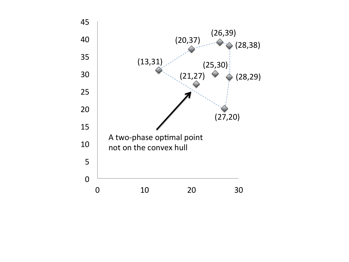
which implies that we can visualize this optimization as that of finding a vertex on the convex hull of points for the weights of - paths in , in a direction determined by and . Moreover, this algorithm cannot find points that are not on the convex hull. (See Figure 4.)

If the values for the edges in are all non-negative, then an optimal -to- path, for any preference pair, , can be found using a standard single-source shortest path algorithm [16], which runs in time, where is the number of vertices in and is the number of edges, by an implementation of Dijkstra’s algorithm (e.g., see [5]). Otherwise, such a path can be found in time, by the Bellman-Ford algorithm (e.g., see [5]). Indeed, for any vertex, , and a given preference pair, , we can use these algorithms to find the tree defined by the union of all -optimal paths in that emanate out from , or are directed into , in these same time bounds. (Note that we may allow such paths to include self-loops at charging stations a finite number of times, so that the topology of their union is still essentially a tree.)
4 Two-Phase Bicriterion Paths
Restriction to finding a route optimizing a single linear utility function, as described above, may be too constraining. Because it misses pairs that are not on the convex hull, if we are planning a route from a source, , to a target, , there might be fast and efficient -to- path, that is missed, since a path minimizing driving time might run out of energy before reaching , while a route minimizing energy consumption might be needlessly slow. (See, for example, Figure 3.) Thus, it would be desirable to consider routes that include a transition from one linear utility function to another at some point, such as a route that optimizes driving time in the beginning of the route and switches to optimizing energy consumption at the end, so as to reach the target vertex quickly without fully discharging the battery.
Suppose we are given two preference pairs, and . For example, we might have , which emphasizes driving time, and , which emphasizes energy consumption. A path, , from to is a two-phase path for and if there is a vertex, , in , such that we can divide into the path, , from to , and the path, , from to , so that is an optimal -to- path for the preference pair and is an optimal -to- path for the preference pair . (For example, in Figure 3, the path is a composition of a time-optimal path from to and an energy-optimal path from to , and this would be a two-phase optimal path for a battery capacity from 27 to 30, inclusive.) As a boundary case, we allow the vertex to be equal to or , so that a single-phase path is just a special case of a two-phase path.
4.1 Finding Two-Phase Paths
In this section, we describe our polynomial-time algorithm for finding an optimal two-phase path from a source, , to a target, , in a graph, , with bicriterion weights on its edges. We describe an algorithm that can search for two-phase paths based on optimizing two out of given preference pairs. Suppose, then, that we are given preference pairs, .
- 1.
For each preference pair, , use the algorithm of Section 3 to find the tree, , that is the union, for all in , of the optimal -to- paths in for the pair . With each node, , store the bicriterion weight, , of the -to- path in .
- 2.
For each preference pair, , use the (reverse) algorithm of Section 3 to find the tree, , that is the union, for all in , of the optimal -to- paths in for the pair . With each node, , store the bicriterion weight, , of the -to- path in .
- 3.
For each node in , and each pair of indices , compute the score
for performing a transition from preference pair to at , where “” is component-wise addition.
- 4.
Search all the values, including values , to find an optimal pair according to the user’s specified optimization goals, such as and , for some and .
We give a schematic illustration of this algorithm in Figure 5.
We note, in addition, that in combining weights in this two-phase manner, we are able to find Pareto-optimal scores that could not be found in any optimization using a single linear utility function. That is, we can find Pareto-optimal scores for paths from to that are not on the convex hull of scores. (See Figure 6.)
Let us analyze the running time of this algorithm. Suppose, first, that there are no negative-weight edges. In this case, we can use Dijkstra’s algorithm to compute each and ; hence, these steps run in time. If, on the other hand, there are negative-weight edges, but no negative cycles, in , then we use a Bellman-Ford algorithm to compute each and ; hence, these steps run in time in this case. Then, computing all the pairs and choosing an optimal such pair takes time. Thus, if is a fixed constant independent of and , then this algorithm runs in time if there are no negative-weight edges and in time otherwise. Note that these running times are asymptotically the same as that of computing an optimal path for a single traversal mode.
In the context of finding electric vehicle routes, each preference pair, , corresponds to a driving style, such as “minimize driving time,” “minimize energy consumption,” or “minimize a weighted combination of driving time and energy consumption.” In addition, the path that achieves the chosen optimal pair, , is simple to implement for the driver of an electric vehicle. He or she simply needs to drive according to driving style from to , that is, using the path in , and then switch to drive according to driving style from to , that is, using the path in .
5 Including Charging Stations
The above two-phase path finding algorithm can be used in the context of negative-weight edges (e.g., where regenerative braking charges the battery, provided we add the capacity constraints as discussed in Section 2). In this case, assuming there are no negative-weight cycles, we could use the Bellman-Ford algorithm to compute the optimal paths, requiring an running time.
If the charging stations themselves are the only places in the network that provide negative energy consumption, then we can achieve a potentially better algorithm for finding good paths. In this case, we consider and to themselves to be charging stations, and we let be the number of charging stations in the network. Moreover, in this case, we assume the user is interested in the shortest duration path from to that can be achieved with a given battery capacity, which starts out fully charged. Also, we assume here that the user fully charges the battery at each charging station at which he or she stops.
With the algorithm we discuss in this section, we can design a long route for an electric vehicle that starts at , and includes several charging stations, fully charging the vehicle at each one along the way, and finally going to , such that we implement a different two-phase path between each pair of charging stations along the way.
- 1.
For each charging station, , and each traversal mode, , use the Dijkstra-type algorithm of Section 3 to find the tree, , that is the union, for all in , of the optimal -to- paths in for the traversal . With each node, , store the bicriterion weight, , of the -to- path in .
- 2.
For each charging station, , and each traversal mode, , use the (reverse) Dijkstra-type algorithm of Section 3 to find the tree, , that is the union, for all in , of the optimal -to- paths in for the traversal . With each node, , store the bicriterion weight, , of the -to- path in .
- 3.
For each pair of charging stations, and , and, for each node in , and each pair of indices , compute the two-phase score,
where “” is component-wise addition.
- 4.
For each pair of charging stations, and , search all the values to find an optimal pair according to the user’s desired goals, to go from to , such as and for given values of and . Create a “super edge,” , from to , and label it with this weight.
- 5.
Create a graph, , whose vertices are charging stations and whose edges are the super edges created in the previous step. For each such super edge, , with weight, , replace this weight with the weight
where is the time needed to charge the battery to add units of energy capacity (and recall that is the capacity of the battery).
- 6.
Use Dijkstra’s algorithm to find a shortest duration path from to in .
We illustrate this algorithm in Figure 7.

Incidentally, if there are negative-weight edges in the graph, but no negative-weight cycles (ignoring charging stations), then we would substitute the Dijkstra-type algorithms used in Steps 1 and 2 for Bellman-Ford-type algorithms.
Let us analyze the running time of this algorithm. To compute all the trees of the form and , using Dijkstra’s algorithm, takes . The time to compute the optimal value for each super edge is , but in practice we only need to consider each pair of charging stations, and , such that is reachable from with a fully charged battery. So the term in this bound might be overly pessimistic. Finally, the final Dijkstra’s algorithm takes at most time, but this is dominated by the running times of the other steps. So the total running time of this algorithm is at most , assuming no negative-weight edges (other than charging stations). Note that if and are fixed constants independent of and , then this running time is , which is asymptotically the same as doing a single Dijkstra-like computation with a single-phase optimization criterion.
If there are negative-weight edges, but no negative-weight cycles, then replacing the Dijkstra-type algorithms in Steps 1 and 2 with Bellman-Ford-type algorithms increases the running time to be , which becomes asymptotically equal to that of a single Bellman-Ford-type computation, i.e., , if and are fixed constants.
6 Experiments
To empirically measure the performance of our algorithms, we tested them using road networks for several U.S. states from the TIGER/Line data sets [28], as prepared for the 9th DIMACS Implementation Challenge [23]. These road networks are undirected, with each edge (road segment) characterized as belonging to one of four general classes: highway, primary major road, secondary major road, or local road. For each road segment of a given class, we consider different driving styles for traversing an edge of that class, allowing for three different speeds at which it can be traveled, in order to capture both lower and upper speed limits inherent to all roads of a certain class. We derived these speeds based on the guidelines presented in the road design manual for the state of Florida [25] (the “Florida greenbook”). For these speed values, see Table 1.
| Road type | Speed | Energy Consumption | |
|---|---|---|---|
| [mph] | [Wh / mile] | ||
| Highway | fast | 70 | 378 |
| moderate | 60 | 329 | |
| slow | 50 | 291 | |
| Primary main road | fast | 70 | 378 |
| moderate | 55 | 308 | |
| slow | 40 | 258 | |
| Secondary main road | fast | 60 | 329 |
| moderate | 45 | 275 | |
| slow | 35 | 221 | |
| Local road | fast | 30 | 202 |
| moderate | 25 | 199 | |
| slow | 20 | 197 | |
Although our algorithms can accommodate elevation changes and even the negative energy consumption that comes from regenerative braking, the data sets in the TIGER/Line collection do not include elevation information; hence, for the sake of simplicity, we assumed in our tests that all roads lie on a flat surface. Extending our testing regime to include elevation data would change some of the weight pairs on some edges in hilly terrains, and would allow for including the second-order effect of elevation, but it would not significantly change the results for reasonably flat terrains.
Moreover, the main goal of our tests was to determine the effectiveness of the two-phase strategy, for which the TIGER/Line data sets were sufficient. In particular, in order to estimate energy consumption for each edge segment, we used the provided edge length and estimated energy consumption based on the data for the Tesla Model S with 85 kWh battery [20, 27] and air conditioning / heating turned on (see also Figure 2). The speed/energy consumption combinations are shown in Table 1. For the two-phase algorithm from Section 4, we considered three driving styles:
- •
emphasize smaller driving time
- •
emphasize smaller energy consumption
- •
balance energy consumption and driving time.
The preference pairs characterizing such paths are shown in Table 2.
| Path type | (time coeff.) | (energy coeff.) |
|---|---|---|
| Fast | 0.8 | 0.2 |
| Balanced | 0.5 | 0.5 |
| Energy-saving | 0.2 | 0.8 |
Rhode Island (, ):
| Capacity | Reachable | Two-phase algorithm | ||
|---|---|---|---|---|
| [Wh] | Nodes | % | Reachability | Longer % |
| 1000 | 2291 | 4.27 % | 100 % | 0.36 % |
| 2000 | 3580 | 6.67 % | 100 % | 0.37 % |
| 4000 | 9824 | 18.31 % | 99.90 % | 1.81 % |
| 6000 | 23482 | 43.76 % | 99.40 % | 2.33 % |
| 8000 | 44815 | 83.52 % | 99.69 % | 3.07 % |
Alaska (, ):
| Capacity | Reachable | Two-phase algorithm | ||
|---|---|---|---|---|
| [Wh] | Nodes | % | Reachability | Longer % |
| 1000 | 2824 | 4.09 % | 100 % | 0.29 % |
| 2000 | 7837 | 11.34 % | 100 % | 0.18 % |
| 4000 | 9497 | 13.75 % | 99.99 % | 0.02 % |
| 6000 | 11306 | 16.37 % | 99.85 % | 0.35 % |
| 8000 | 12129 | 17.56 % | 99.99 % | 0.25 % |
| 10000 | 13335 | 19.30 % | 99.50 % | 0.80 % |
| 12000 | 17658 | 25.56 % | 99.56 % | 2.36 % |
Delaware (, ):
| Capacity | Reachable | Two-phase algorithm | ||
|---|---|---|---|---|
| [Wh] | Nodes | % | Reachability | Longer % |
| 1000 | 3970 | 8.08 % | 100 % | 0.53 % |
| 2000 | 12249 | 24.94 % | 100 % | 1.43 % |
| 4000 | 18154 | 36.97 % | 99.99 % | 0.09 % |
| 6000 | 19875 | 40.47 % | 99.98 % | 0.18 % |
| 8000 | 21252 | 43.28 % | 99.98 % | 0.10 % |
| 10000 | 23113 | 47.06 % | 99.84 % | 0.13 % |
| 12000 | 26656 | 54.28 % | 99.87 % | 0.28 % |
| 14000 | 28783 | 58.61 % | 99.87 % | 0.37 % |
| 16000 | 31381 | 63.90 % | 99.80 % | 0.29 % |
District of Columbia (, ):
| Capacity | Reachable | Two-phase algorithm | ||
|---|---|---|---|---|
| [Wh] | Nodes | % | Reachability | Longer % |
| 1000 | 3370 | 35.25 % | 99.97 % | 3.20 % |
| 2000 | 8353 | 87.39 % | 99.96 % | 4.74 % |
| 4000 | 9522 | 99.61 % | 100 % | 0.76 % |
6.1 Quality of Paths
As we argue above, the real-world goal of people driving electric vehicles is to find a path that leads to the destination in the smallest amount of time while ensuring that the battery stays at least partially charged at all points along the way [9, 10, 13]. To measure the quality of the two-phase bicriterion algorithm of Section 4, we compared the paths it returns against the optimal paths (that arrive at reachable destinations in shortest time) found by the pseudo-polynomial time algorithm of Section 2, where we set to be the capacity (in Wh) of the battery.
Due to the time complexity needed for finding optimal paths using the vertex-labeling algorithm, we were only able to compare the two algorithms on smaller graphs (with ), representing small states (like Rhode Island, Delaware or the District of Columbia) or large states with sparse road network (Alaska). In addition, due to time constraints imposed by the slow running time of the vertex-labeling algorithm, we also did not consider placing charging stations in the graphs for these comparison tests.
The results are shown in Table 3 and Figure 8, comparing the paths found by our algorithm with the optimal paths found by the vertex-labeling algorithm. Due to high running times for the vertex-labeling algorithm (which depend in a pseudo-polynomial fashion on battery capacity), we restricted battery capacity to values much smaller than the actual 60 kWh (or 85 kWh) for the Tesla Model S. These capacities are shown in the first column of Table 3. In the second and third column, we show the number of nodes reachable by the vertex-labeling algorithm, both in absolute numbers and as a percentage of all nodes in the network. The next column shows the percentage of the (optimally) reachable nodes that can be reached by the two-phase algorithm. The final column depicts the average slowdown of the paths computed by the two-phase algorithm relative to the optimal paths.
California (, ):
| Capacity [Wh] | Chargers | Reachability | Time [s] |
|---|---|---|---|
| 60000 | 0 | 55.2 % | 12.80 |
| 60000 | 1 | 56.2 % | 24.63 |
| 60000 | 2 | 56.2 % | 33.37 |
| 60000 | 3 | 95.3 % | 53.98 |
| 60000 | 4 | 96.2 % | 73.04 |
| 60000 | 5 | 97.6 % | 91.39 |
| 85000 | 0 | 70.7 % | 21.38 |
| 85000 | 1 | 77.0 % | 28.26 |
| 85000 | 2 | 98.3 % | 43.01 |
Alaska (, ):
| Capacity [Wh] | Chargers | Reachability | Time [s] |
|---|---|---|---|
| 60000 | 0 | 29.2 % | 0.48 |
| 60000 | 2 | 39.5 % | 1.01 |
| 60000 | 5 | 40.8 % | 2.03 |
| 60000 | 13 | 40.9 % | 6.94 |
| 60000 | 14 | 43.3 % | 7.70 |
| 60000 | 15 | 47.7 % | 8.59 |
| 85000 | 0 | 43.6 % | 0.48 |
| 85000 | 2 | 47.6 % | 1.11 |
| 85000 | 13 | 47.7 % | 7.86 |
| 85000 | 15 | 47.8 % | 9.84 |
Montana (, ):
| Capacity [Wh] | Chargers | Reachability | Time [s] |
|---|---|---|---|
| 60000 | 0 | 88.3 % | 9.90 |
| 60000 | 1 | 88.4 % | 12.83 |
| 60000 | 2 | 96.1 % | 18.46 |
| 60000 | 3 | 96.7 % | 22.39 |
| 60000 | 6 | 97.5 % | 39.00 |
| 60000 | 7 | 97.9 % | 57.42 |
| 85000 | 0 | 97.0 % | 9.93 |
| 85000 | 1 | 97.3 % | 14.01 |
| 85000 | 2 | 98.2 % | 20.33 |
Texas (, ):
| Capacity [Wh] | Chargers | Reachability | Time [s] |
|---|---|---|---|
| 60000 | 0 | 47.2 % | 22.83 |
| 60000 | 1 | 49.8 % | 26.55 |
| 60000 | 2 | 56.1 % | 49.86 |
| 60000 | 3 | 57.9 % | 64.33 |
| 60000 | 4 | 58.4 % | 89.50 |
| 60000 | 5 | 69.2 % | 113.34 |
| 60000 | 7 | 69.3 % | 154.51 |
| 60000 | 9 | 71.2 % | 190.46 |
| 85000 | 0 | 68.7 % | 28.73 |
| 85000 | 1 | 75.1 % | 35.10 |
| 85000 | 2 | 80.6 % | 58.75 |
| 85000 | 3 | 82.4 % | 86.36 |
| 85000 | 5 | 94.9 % | 138.59 |
Nevada (, ):
| Capacity [Wh] | Chargers | Reachability | Time [s] |
|---|---|---|---|
| 60000 | 0 | 55.7 % | 2.87 |
| 60000 | 1 | 63.2 % | 4.81 |
| 60000 | 2 | 67.9 % | 6.43 |
| 60000 | 4 | 81.9 % | 11.62 |
| 60000 | 10 | 92.6 % | 34.06 |
| 85000 | 0 | 80.6 % | 3.44 |
| 85000 | 1 | 92.6 % | 5.99 |
6.2 Performance
As mentioned above, due to the extremely large running time of the optimal pseudo-polynomial algorithm (for the largest instances our runs exceeded 24 hours), we were forced to restrict our qualitative testing to road networks of small states, and use unrealistically small battery capacities. In this subsection, we focus on the performance of the two-phase algorithm, which, thanks to its superior time complexity, allows us to meet the following goals:
- •
Use actual capacities of Tesla Model S (60/85 kWh).
- •
Include charging stations.
- •
Test the algorithm on larger graphs.
Under the above assumptions, we measured the running time of the algorithm, as well as estimated the reachability percentage (measured as a ratio of feasible paths between pairs of randomly chosen vertices and the total number of pairs tested; in each case, we tested 1000 pairs). The results are summarized in Table 4, Table 5, Figure 9 and Figure 10. The times shown in the last column is the average duration of a single execution of the two-phase algorithm. Charging stations were placed at randomly selected vertices. Only instances that actually increased reachability are shown.
6.3 Discussion
Tests were implemented in C++ and carried out on a PC with a 2.2 GHz CPU, 1066 MHz bus, and 4 GB RAM running Linux. It is evident that the two-phase algorithm finds paths to almost all reachable destinations, with the paths being only slightly slower (taking more time) that the optimal ones.
Our results were obtained using the following procedure: for each state, we randomly chose a starting position and 1000 destinations. It gave us 1000 origin-destination pairs, on which we then tested the algorithms described above. The resolution of our algorithms was: seconds (for time) and Wh (for energy).
Our implementation of the two-phase algorithm is straightforward. We did not optimize it for running time and we deliberately ran it on a relatively old PC, and, admittedly, this shows in the results. Even then, the algorithm was able to compute paths within several dozens of seconds. Since the number of charging stations is the main factor in running time, one optimization would be to precompute best paths between all pairs of charging stations (which is feasible, as the number of charging stations is small and they are fixed features of a road network). The running time of the algorithm would then be reduced to the case of no charging stations. As the main component of our procedure is the Dijkstra’s shortest path algorithm, another straightforward improvement would be to incorporate some of existing approaches [7, 6] aimed at speeding up Dijkstra’s algorithm.
7 Conclusion
We have presented a two-phase approach for finding good paths in bicriterion networks, and we have demonstrated that our algorithms are both fast and effective for finding good routes for electric vehicles. In particular, we have shown empirically that the paths found by the two-phase algorithm can identify over 99% of the vertices reachable in a road network by some energy-efficient algorithm, while being only slightly longer on average than paths found by the inefficient vertex-labeling algorithm. Moreover, we believe that two-phase are easier for people to follow, since, in addition to the route they plan to take, they only need to remember two different driving styles and the point in the route where they transition from the first driving style to the second. Of course, if charging stations are involved, it may require style transitions. This is usually not a problem, since common trips tend to use a small number of charging station located far away.
As possible future work, it would be interesting to test the two-phase approach for finding good delivery routes for electric vehicles that have multiple destinations.
Acknowledgments
This work was supported in part by the NSF, under grant 1011840 and 1228639, and by the Office of Naval Research, under grant N00014-08-1-1015. We would like to thank David Eppstein and Amelia Regan for several helpful communications regarding the topics of this paper.
References
- [1] E. M. Arkin, J. S. Mitchell, and C. D. Piatko. Bicriteria shortest path problems in the plane. In Proc. 3rd Canad. Conf. Comput. Geom, pages 153–156, 1991.
- [2] A. Artmeier, J. Haselmayr, M. Leucker, and M. Sachenbacher. The shortest path problem revisited: Optimal routing for electric vehicles. In R. Dillmann, J. Beyerer, U. Hanebeck, and T. Schultz, editors, Advances in Artificial Intelligence, volume 6359 of LNCS, pages 309–316. Springer, 2010.
- [3] M. Baum, J. Dibbelt, T. Pajor, and D. Wagner. Energy-optimal routes for electric vehicles. In 21st ACM SIGSPATIAL Int. Conf. on Adv. in Geographic Information Systems, pages 54–63, 2013.
- [4] J. C. N. Climaco and E. Q. V. Martins. A bicriterion shortest path algorithm. European Journal of Operational Research, 11(4):399–404, 1982.
- [5] T. H. Cormen, C. E. Leiserson, R. L. Rivest, and C. Stein. Introduction to Algorithms. MIT Press, Cambridge, MA, 2nd edition, 2001.
- [6] D. Delling, A. V. Goldberg, T. Pajor, and R. F. F. Werneck. Customizable route planning. In P. M. Pardalos and S. Rebennack, editors, SEA, volume 6630 of Lecture Notes in Computer Science, pages 376–387. Springer, 2011.
- [7] D. Delling, P. Sanders, D. Schultes, and D. Wagner. Engineering route planning algorithms. In J. Lerner, D. Wagner, and K. A. Zweig, editors, Algorithmics of Large and Complex Networks, volume 5515 of Lecture Notes in Computer Science, pages 117–139. Springer, 2009.
- [8] J. Eisner, S. Funke, and S. Storandt. Optimal route planning for electric vehicles in large networks. In AAAI, 2011.
- [9] T. Franke and J. F. Krems. What drives range preferences in electric vehicle users? Transport Policy, 30(0):56–62, 2013.
- [10] T. Franke, I. Neumann, F. Bühler, P. Cocron, and J. F. Krems. Experiencing range in an electric vehicle: Understanding psychological barriers. Applied Psychology, 61(3):368–391, 2012.
- [11] M. R. Garey and D. S. Johnson. Computers and Intractability: A Guide to the Theory of NP-Completeness. W. H. Freeman, New York, NY, 1979.
- [12] A. V. Goldberg, H. Kaplan, and R. F. Werneck. Reach for : Efficient point-to-point shortest path algorithms. In Proc. 8th Workshop on Algorithm Engineering and Experiments (ALENEX), pages 129–143, 2006.
- [13] E. Graham-Rowe, B. Gardner, C. Abraham, S. Skippon, H. Dittmar, R. Hutchins, and J. Stannard. Mainstream consumers driving plug-in battery-electric and plug-in hybrid electric cars: A qualitative analysis of responses and evaluations. Transportation Research Part A: Policy and Practice, 46(1):140–153, 2012.
- [14] P. Hansen. Bicriterion path problems. In G. Fandel and T. Gal, editors, Multiple Criteria Decision Making Theory and Application, volume 177 of Lecture Notes in Economics and Mathematical Systems, pages 109–127. Springer, 1980.
- [15] R. Hassin. Approximation schemes for the restricted shortest path problem. Mathematics of Operations Research, 17(1):36–42, 1992.
- [16] M. I. Henig. The shortest path problem with two objective functions. European Journal of Operational Research, 25(2):281–291, 1986.
- [17] K. Mehlhorn and M. Ziegelmann. Resource constrained shortest paths. In M. S. Paterson, editor, European Symp. on Algorithms (ESA), volume 1879 of LNCS, pages 326–337. Springer, 2000.
- [18] P. Modesti and A. Sciomachen. A utility measure for finding multiobjective shortest paths in urban multimodal transportation networks. European Journal of Operational Research, 111(3):495–508, 1998.
- [19] J. Mote, I. Murthy, and D. L. Olson. A parametric approach to solving bicriterion shortest path problems. European Journal of Operational Research, 53(1):81–92, 1991.
- [20] E. Musk and J. B. Straubel. Model S efficiency and range, 2012. http://www.teslamotors.com/blog/model-s-efficiency-and-range.
- [21] G. Righini and M. Salani. Symmetry helps: Bounded bi-directional dynamic programming for the elementary shortest path problem with resource constraints. Discrete Optimization, 3(3):255–273, 2006.
- [22] M. Sachenbacher, M. Leucker, A. Artmeier, and J. Haselmayr. Efficient energy-optimal routing for electric vehicles. In AAAI, 2011.
- [23] D. Schultes. 9th DIMACS Implementation Challenge files, October 2005. http://www.dis.uniroma1.it/challenge9/data/tiger.
- [24] A. Skriver and K. Andersen. A label correcting approach for solving bicriterion shortest-path problems. Computers & Operations Research, 27(6):507–524, 2000.
- [25]
State of Florida, Department of Transportation.
Manual of uniform minimum standards for design, construction and
maintenance for streets and highways.
May 2011.
http://www.dot.state.fl.us/rddesign/
FloridaGreenbook/FGB.shtm. - [26] S. Storandt. Quick and energy-efficient routes: Computing constrained shortest paths for electric vehicles. In 5th ACM SIGSPATIAL Int. Workshop on Computational Transportation Science (IWCTS), pages 20–25, 2012.
- [27] Tesla Motors. Your questions answered, 2014. http://www.teslamotors.com/goelectric.
- [28] U.S. Census Bureau. Redistricting census 2000 TIGER/Line files [machine-readable data files], 2000.