跳到论文正文
W Papers独立论文阅读器 arXiv:1409.2849 论文正文 计算阅读时间 · 0%
引用这篇论文根据当前论文元数据生成,正式投稿前建议核对。


License: arXiv.org perpetual non-exclusive license
arXiv:1409.2849v1 [math.PR] 09 Sep 2014

Mod-Gaussian convergence and its applications
for models of statistical mechanics

Pierre-Loïc Méliot and Ashkan Nikeghbali In memoriam, Marc Yor.
Date: August 24, 2026
Abstract.

In this paper we complete our understanding of the role played by the limiting (or residue) function in the context of mod-Gaussian convergence. The question about the probabilistic interpretation of such functions was initially raised by Marc Yor. After recalling our recent result which interprets the limiting function as a measure of "breaking of symmetry" in the Gaussian approximation in the framework of general central limit theorems type results, we introduce the framework of L1\mathrm{L}^{1}-mod-Gaussian convergence in which the residue function is obtained as (up to a normalizing factor) the probability density of some sequences of random variables converging in law after a change of probability measure. In particular we recover some celebrated results due to Ellis and Newman on the convergence in law of dependent random variables arisisng in statistical mechanics. We complete our results by giving an alternative approach to the Stein method to obtain the rate of convergence in the Ellis-Newman convergence theorem and by proving a new local limit theorem. More generally we illustrate our results with simple models from statistical mechanics.

1. Introduction

Let (Xn)n∈ℕ(X_{n})_{n\in\mathbb{N}} be a sequence of real-valued random variables. In the series of papers [JKN11, DKN11, KN10, KN12, FMN13], we introduced the notion of mod-Gaussian convergence (and more generally of mod-convergence with respect to an infinitely divisible law ϕ\phi):

Definition 1.

The sequence (Xn)n∈ℕ(X_{n})_{n\in\mathbb{N}} is said to converge in the mod-Gaussian sense with parameters tn→+∞t_{n}\to+\infty and limiting (or residue) function θ\theta if, locally uniformly in ℝ\mathbb{R},

𝔼⁡[ei​t​Xn]​etn​t22=θ⁡(t)​(1+o⁡(1)),\mathbb{E}[\mathrm{e}^{\mathrm{i}tX_{n}}]\,\mathrm{e}^{\frac{t_{n}\,t^{2}}{2}}=\theta(t)\,(1+o(1)),

where θ\theta is a continuous function on ℝ\mathbb{R} with θ⁡(0)=1\theta(0)=1.

A trivial situation of mod-Gaussian convergence is when Xn=Gn+YnX_{n}=G_{n}+Y_{n} is the sum of a Gaussian variable of variance tnt_{n} and of an independent random variable YnY_{n} that converges in law to a variable YY with characteristic function θ\theta. More generally XnX_{n} can be thought of as a Gaussian variable of variance tnt_{n}, plus a noise which is encoded by the multiplicative residue θ\theta in the characteristic function. In this setting, θ\theta is not necessarily the characteristic function of a random variable (the residual noise). For instance, consider

Xn=1n1/3​∑i=1nYi,X_{n}=\frac{1}{n^{1/3}}\sum_{i=1}^{n}Y_{i},

where the YiY_{i} are centred, independent and identically distributed random variables with convergent moment generating function. Then a Taylor expansion of 𝔼⁡[ei​t​Y]\mathbb{E}[\mathrm{e}^{\mathrm{i}tY}] shows that (Xn)n∈ℕ(X_{n})_{n\in\mathbb{N}} converges in the mod-Gaussian sense with parameters n1/3​Var​(Y)n^{1/3}\,\mathrm{Var}(Y) and limiting function

θ⁡(t)=exp⁡(𝔼⁡[Y3]​(i​t)36),\theta(t)=\exp\left(\frac{\mathbb{E}[Y^{3}]\,(\mathrm{i}t)^{3}}{6}\right),

which is not the characteristic function of a random variable, since it does not go to zero as tt goes to infinity. In 2008, during the workshop "Random matrices, L-functions and primes" held in Zürich, Marc Yor asked the second author A. N. about the role of the limiting function θ\theta. In [KNN13] it is proved that the set of possible limiting functions is the set of continuous functions θ\theta from ℝ\mathbb{R} to ℂ\mathbb{C} such that θ⁡(0)=1\theta(0)=1 and θ​(−t)=θ¯​(t)\theta(-t)=\bar{\theta}(t) for t∈ℝt\in\mathbb{R}. But this characterization does not say anything on the probabilistic information encoded in θ\theta. We now wish to develop more on probabilistic interpretations of the limiting function and the implications of mod-Gaussian convergence in terms of classical limit theorems of probability theory.

We first note that by looking at 𝔼⁡[ei​t​Xn/tn]\mathbb{E}[\mathrm{e}^{\mathrm{i}tX_{n}/\sqrt{t_{n}}}], one immediately sees that mod-Gaussian convergence implies a central limit theorem for the sequence (Xntn)(\frac{X_{n}}{\sqrt{t_{n}}}):

(1) Xntn⇀n→∞𝒩(0,1),\frac{X_{n}}{\sqrt{t_{n}}}\rightharpoonup_{n\to\infty}\mathcal{N}(0,1),

where the convergence above holds in law (see [JKN11, §2-3] for more details on this). On the other hand, with somewhat stronger hypotheses on the remainder o⁡(1)o(1) that appears in Definition 1, a local limit theorem also holds, see [KN12, Theorem 4] and [DKN11, Theorem 5]:

ℙ[Xn∈B]=ℙ[Gn∈B](1+o(1))=m⁡(B)2​π​tn(1+o(1))\mathbb{P}[X_{n}\in B]=\mathbb{P}[G_{n}\in B]\,(1+o(1))=\frac{m(B)}{\sqrt{2\pi t_{n}}}\,(1+o(1))

for relatively compact sets BB with m⁡(∂B)=0m(\partial B)=0, mm denoting the Lebesgue measure.

In [FMN13], it is then explained that by looking at Laplace transforms instead of characteristic functions, and by assuming the convergence holds on a whole band of the complex plane, one can obtain in the setting of mod-Gaussian convergence precise estimates of moderate or large deviations. In fact these results provide a new probabilistic interpretation of the limiting function as a measure of the "breaking of symmetry" in the Gaussian approximation of the tails of XnX_{n} (see §1.1 for more details).

The goal of this paper is threefold:

  • •

    to propose a new interpretation of the limiting function in the framework of mod-Gaussian convergence with Laplace transforms; these results allow us in particular to recover some well known exotic limit theorems from statistical mechanics due to Ellis and Newman [EN78] and similar one for other models or in higher dimensions.

  • •

    to show that once one is able to prove mod-Gaussian convergence, then one can expect to obtain finer results than merely convergence in law, such as speed of convergence and local limit theorems. Results on the rate of convergence in the Curie-Weiss model were recently obtained using Stein’s method (see e.g. [EL10]) while the local limit theorem, to the best of our knowledge, is new.

  • •

    to explore the applications of the results obtained in [FMN13] on the "breaking of symmetry" in the central limit theorem to some classical models of statistical mechanics. In particular our approach determines the scale up to which the Gaussian approximation for the tails is valid and its breaking at this critical scale.

Our results are best illustrated with some classical one-dimensional models from statistical mechanics, such as the Curie-Weiss model or the Ising model. To illustrate the flexibility of our approach, we shall also prove similar results for weighted symmetric random walks in dimensions 22 and 33. The statistics of interest to us will be the total magnetization, which can be written as a sum of dependent random variables. These examples add to the already large class of examples of sums of dependent random variables we have already been able to deal with in the context of mod-ϕ\phi convergence.

In the remaining of the introduction we recall the results obtained in [FMN13] which led us to the "breaking of symmetry" interpretation, as well as an underlying method of cumulants that enabled us to establish the mod-Gaussian convergence for a large family of sums of dependent random variables. The important aspect of the cumulant method is that it provides a tool to prove mod-Gaussian convergence in situations where one cannot explicitly compute the characteristic function. We eventually give an outline of the paper.

1.1. Complex convergence and interpretation of the residue

We consider again a sequence of real-valued random variables (Xn)n∈ℕ(X_{n})_{n\in\mathbb{N}}, but this time we assume that their Laplace transforms 𝔼⁡[ez​Xn]\mathbb{E}[\mathrm{e}^{zX_{n}}] are convergent in an open disk of radius c>0c>0. In this case, they are automatically well-defined and holomorphic in a band of the complex plane ℬc={z∈ℂ,|Re⁡(z)|<c}\mathcal{B}_{c}=\{z\in\mathbb{C},\,\,|\mathrm{Re}(z)|<c\} (see [LS52, Theorem 6], and [Ess45] for a general survey of the properties of Laplace and Fourier transforms of probability measures).

Definition 2.

The sequence (Xn)n∈ℕ(X_{n})_{n\in\mathbb{N}} is said to converge in the complex mod-Gaussian sense with parameters tnt_{n} and limiting function ψ\psi if, locally uniformly on ℬc\mathcal{B}_{c},

𝔼⁡[ez​Xn]​e−tn​z22=ψ⁡(z)​(1+o⁡(1)),\mathbb{E}[\mathrm{e}^{zX_{n}}]\,\mathrm{e}^{-\frac{t_{n}\,z^{2}}{2}}=\psi(z)\,(1+o(1)),

where ψ\psi is a continuous function on ℬc\mathcal{B}_{c} with ψ⁡(0)=1\psi(0)=1. Then, one has in particular convergence in the sense of Definition 1, with θ⁡(t)=ψ⁡(i​t)\theta(t)=\psi(\mathrm{i}t).

In this setting which is more restrictive than before, the residue ψ\psi has a natural interpretation as a measure of "breaking of symmetry" when one tries to push the estimates of the central limit theorem from the scale tn\sqrt{t_{n}} to the scale tnt_{n}. The previously mentioned central limit theorem (1) tells us that:

ℙ[Xn≥atn]=(12​π∫a∞e−x22dx)(1+o(1))\mathbb{P}\!\left[X_{n}\geq a\sqrt{t_{n}}\right]=\left(\frac{1}{\sqrt{2\pi}}\int_{a}^{\infty}\mathrm{e}^{-\frac{x^{2}}{2}}\,dx\right)(1+o(1))

for any a∈ℝa\in\mathbb{R}. In the setting of complex mod-Gaussian convergence, this estimate remains true with a=o⁡(tn)a=o(\sqrt{t_{n}}), so that if ε=o⁡(1)\varepsilon=o(1), then

ℙ[Xn≥εtn]\displaystyle\mathbb{P}\left[X_{n}\geq\varepsilon\,t_{n}\right] =(12​π​∫ε​tn∞e−x22​𝑑x)​(1+o⁡(1)),\displaystyle=\left(\frac{1}{\sqrt{2\pi}}\int_{\varepsilon\sqrt{t_{n}}}^{\infty}\mathrm{e}^{-\frac{x^{2}}{2}}\,dx\right)(1+o(1)),
=e−tn​ε222​π​tn​ε​(1+o⁡(1)) if ​1≫ε≫1tn,\displaystyle=\frac{\mathrm{e}^{-\frac{t_{n}\varepsilon^{2}}{2}}}{\sqrt{2\pi t_{n}}\,\varepsilon}\,(1+o(1))\quad\text{ if }1\gg\varepsilon\gg\frac{1}{\sqrt{t_{n}}}\,,

where the notation an≫bna_{n}\gg b_{n} stands for bn=o⁡(an)b_{n}=o(a_{n}). Then, at scale tnt_{n}, the limiting residue ψ\psi comes into play, with the following estimate that holds without additional hypotheses than those in Definition 2:

(2) ∀x∈(0,c),ℙ[Xn≥xtn]=e−tn​x222​π​tn​xψ(x)(1+o(1)),\forall x\in(0,c),\,\,\,\mathbb{P}[X_{n}\geq xt_{n}]=\frac{\mathrm{e}^{-\frac{t_{n}x^{2}}{2}}}{\sqrt{2\pi t_{n}}\,x}\,\psi(x)\,(1+o(1)),

the remainder o⁡(1)o(1) being uniform when xx stays in a compact set of ℝ+∗∩(0,c)\mathbb{R}_{+}^{*}\cap(0,c). This estimate of positive large deviations has the following counterpart on the negative side:

∀x∈(0,c),ℙ[Xn≤−xtn]=e−tn​x222​π​tn​xψ(−x)(1+o(1)).\forall x\in(0,c),\,\,\,\mathbb{P}[X_{n}\leq-xt_{n}]=\frac{\mathrm{e}^{-\frac{t_{n}x^{2}}{2}}}{\sqrt{2\pi t_{n}}\,x}\,\psi(-x)\,(1+o(1)).

So for instance, if (Yn)n∈ℕ(Y_{n})_{n\in\mathbb{N}} is a sequence of i.i.d. random variables with convergent moment generating function, mean 00, variance 11 and third moment 𝔼⁡[Y]>0\mathbb{E}[Y]>0, then Xn=1n1/3​∑i=1nYiX_{n}=\frac{1}{n^{1/3}}\sum_{i=1}^{n}Y_{i} converges in the complex mod-Gaussian sense with parameters n1/3n^{1/3} and limiting function ψ⁡(z)=exp⁡(𝔼⁡[Y3]​z3/6)\psi(z)=\exp(\mathbb{E}[Y^{3}]\,z^{3}/6), and therefore for x>0x>0,

ℙ[∑i=1nYi≥xn2/3]=ℙ[𝒩(0,1)≥xn1/6]exp(𝔼⁡[Y3]​x36)(1+o(1)).\mathbb{P}\!\left[\sum_{i=1}^{n}Y_{i}\geq xn^{2/3}\right]=\mathbb{P}\!\left[\mathcal{N}(0,1)\geq xn^{1/6}\right]\,\,\exp\!\left(\frac{\mathbb{E}[Y^{3}]\,x^{3}}{6}\right)\,(1+o(1)).

Thus, at scale n2/3n^{2/3}, the fluctuations of the sum of i.i.d. random variables are no more Gaussian, and the residue ψ⁡(x)\psi(x) measures this "breaking of symmetry": in the previous example, it makes moderate deviations on the positive side more likely than moderate deviations on the negative side, since ψ⁡(x)>1>ψ⁡(−x)\psi(x)>1>\psi(-x) for x>0x>0.

Remark.

The problem of finding the normality zone, i.e. the scale up to which the central limit theorem is valid, is a known problem in the case of i.i.d. random variables (see e.g. [IL71]). The description of the "symmetry breaking" is new and moreover the mod-Gaussian framework covers many examples with dependent random variables (see also [FMN13] for more examples).

Thus, the observation of large deviations of the random variables XnX_{n} provides a first probabilistic interpretation of the residue ψ\psi in the deconvolution of a sequence of characteristic functions of random variables by a sequence of large Gaussian variables. In Section 3, we shall provide another interpretation of ψ\psi, which is inspired by some classical results from statistical mechanics (cf. [EN78, ENR80]).

1.2. The method of joint cumulants

The appearance of an exponential of a monomial K​xr≥3Kx^{r\geq 3} as the limiting residue in mod-Gaussian convergence is a phenomenon that occurs not only for sums of i.i.d. random variables, but more generally for sums of possibly non identically distributed and/or dependent random variables. For instance,

  1. (1)

    the number of zeroes of a random Gaussian analytic function ∑k=0∞(𝒩ℂ)k​zk\sum_{k=0}^{\infty}(\mathcal{N}_{\mathbb{C}})_{k}\,z^{k} in the disk of radius 1−1n1-\frac{1}{n};

  2. (2)

    the number of triangles in a random Erdös-Rényi graph G⁡(n,p)G(n,p);

are both mod-Gaussian convergent after proper rescaling, and with limiting function of the form exp⁡(L​z3)\exp(Lz^{3}), with the constant LL depending on the model (see again [FMN13]). The reason behind these universal asymptotics lies in the following method of cumulants. If XX is a random variable with convergent Laplace transform 𝔼⁡[ez​X]\mathbb{E}[\mathrm{e}^{zX}] on a disk, we recall that its cumulant generating function is

(3) log⁡𝔼⁡[ez​X]=∑r≥1κ(r)​(X)r!​zr,\log\mathbb{E}[\mathrm{e}^{zX}]=\sum_{r\geq 1}\frac{\kappa^{(r)}(X)}{r!}\,z^{r},

which is also well-defined and holomorphic on a disk around the origin. Its coefficients κ(r)​(X)\kappa^{(r)}(X) are the cumulants of the variable XX, and they are homogenenous polynomials in the moments of XX; for instance, κ(1)​(X)=𝔼​[X]\kappa^{(1)}(X)=\mathbb{E}[X], κ(2)​(X)=𝔼⁡[X2]−𝔼​[X]2\kappa^{(2)}(X)=\mathbb{E}[X^{2}]-\mathbb{E}[X]^{2}, and κ(3)​(X)=𝔼⁡[X3]−3​𝔼​[X2]​𝔼​[X]+2​𝔼​[X]3\kappa^{(3)}(X)=\mathbb{E}[X^{3}]-3\,\mathbb{E}[X^{2}]\,\mathbb{E}[X]+2\,\mathbb{E}[X]^{3}.

Consider now a sequence of random variables (Wn)n∈ℕ(W_{n})_{n\in\mathbb{N}} with κ(1)​(Wn)=0\kappa^{(1)}(W_{n})=0, and for r≥2r\geq 2,

(4) κ(r)​(Wn)=Kr​αn​(1+o⁡(1)),\kappa^{(r)}(W_{n})=K_{r}\,\alpha_{n}\,(1+o(1)),

with αn→+∞\alpha_{n}\to+\infty. This assumption is inspired by the case of a sum Wn=∑i=1nYiW_{n}=\sum_{i=1}^{n}Y_{i} of centred i.i.d. random variables for which κr​(Wn)=n​κ(r)​(Y)\kappa^{r}(W_{n})=n\,\kappa^{(r)}(Y). If it is satisfied, then one can formally write

log\displaystyle\log 𝔼⁡[ez​Wn(αn)1/3]\displaystyle\,\mathbb{E}\!\left[\mathrm{e}^{z\,\frac{W_{n}}{(\alpha_{n})^{1/3}}}\right]
=(αn)−2/3κ(2)​(Wn)​z22+(αn)−1κ(3)​(Wn)​z36+∑r≥4κ(r)​(Wn)r!((αn)−1/3z)r\displaystyle=(\alpha_{n})^{-2/3}\,\frac{\kappa^{(2)}(W_{n})\,z^{2}}{2}+(\alpha_{n})^{-1}\,\frac{\kappa^{(3)}(W_{n})\,z^{3}}{6}+\sum_{r\geq 4}\frac{\kappa^{(r)}(W_{n})}{r!}((\alpha_{n})^{-1/3}z)^{r}
≃(αn)1/3​K2​z22+K3​z36+∑r≥4Kr​zrr!​(αn)1−r/3\displaystyle\simeq(\alpha_{n})^{1/3}\,\frac{K_{2}\,z^{2}}{2}+\frac{K_{3}\,z^{3}}{6}+\sum_{r\geq 4}\frac{K_{r}\,z^{r}}{r!}(\alpha_{n})^{1-r/3}
≃(αn)1/3​K2​z22+K3​z36\displaystyle\simeq(\alpha_{n})^{1/3}\,\frac{K_{2}\,z^{2}}{2}+\frac{K_{3}\,z^{3}}{6}

whence the mod-Gaussian convergence of Xn=(αn)−1/3WnX_{n}=(\alpha_{n})^{-1/3}\,W_{n}, with parameters tn=K2​(αn)1/3t_{n}=K_{2}\,(\alpha_{n})^{1/3} and limiting function exp⁡(K3​z3/6)\exp(K_{3}\,z^{3}/6). The approximation is valid if the o⁡(1)o(1) in the asymptotics of κ(2)​(Wn)\kappa^{(2)}(W_{n}) is small enough (namely o((αn)−1/3)o((\alpha_{n})^{-1/3})), and if the series ∑r≥4\sum_{r\geq 4} can be controlled, which is the case if

(5) ∀r,|κ(r)​(Wn)|≤(C​r)r​αn\forall r,\,\,|\kappa^{(r)}(W_{n})|\leq(Cr)^{r}\,\alpha_{n}

for some constant CC. The method of cumulants in the setting of mod-Gaussian convergence amounts to prove (4) for the first cumulants of the sequence (Xn)n∈ℕ(X_{n})_{n\in\mathbb{N}}, and (5) for all the other cumulants. From such estimates one then obtains mod-Gaussian convergence for an appropriate renormalisation of (Wn)r≥3(W_{n})_{r\geq 3}, with limiting function exp⁡(Kr​zr/r!)\exp(K_{r}\,z^{r}/r!), where rr is the smallest integer greater or equal than 33 such that Kr≠0K_{r}\neq 0.

This method of cumulants works well with sequences (Wn)n∈ℕ(W_{n})_{n\in\mathbb{N}} that write as sums of (weakly) dependent random variables. Indeed, cumulants admit the following generalization to families of random variables, see [LS59]. Denote 𝔔r\mathfrak{Q}_{r} the set of partitions of [[1,r]]={1,2,3,…,r}\left[\!\left[1,r\right]\!\right]=\{1,2,3,\ldots,r\}, and μ\mu the Möbius function of this poset (see [Rot64] for basic facts about Möbius functions of posets):

μ⁡(Π)=(−1)ℓ⁡(Π)−1​(ℓ⁡(Π)−1)!\mu(\Pi)=(-1)^{\ell(\Pi)-1}\,(\ell(\Pi)-1)!

where ℓ⁡(Π)=s\ell(\Pi)=s if Π=π1⊔π2⊔⋯⊔πs\Pi=\pi_{1}\sqcup\pi_{2}\sqcup\cdots\sqcup\pi_{s} has ss parts. The joint cumulant of a family of rr random variables with well defined moments of all order is

κ⁡(X1,…,Xr)=∑Π∈𝔔rμ⁡(Π)​∏i=1ℓ⁡(Π)𝔼⁡[∏j∈πiXj].\kappa(X_{1},\ldots,X_{r})=\sum_{\Pi\in\mathfrak{Q}_{r}}\mu(\Pi)\,\prod_{i=1}^{\ell(\Pi)}\mathbb{E}\!\left[\prod_{j\in\pi_{i}}X_{j}\right].

It is multilinear and generalizes Equation (3), since

κ⁡(X1,…,Xr)\displaystyle\kappa(X_{1},\ldots,X_{r}) =∂r∂z1∂z2⋯∂zr|z1=⋯=zr=0​(log⁡𝔼⁡[ez1​X1+⋯+zr​Xr])\displaystyle=\left.\frac{\partial^{r}}{\partial z_{1}\partial z_{2}\cdots\partial z_{r}}\right|_{z_{1}=\cdots=z_{r}=0}\big(\log\mathbb{E}[\mathrm{e}^{z_{1}X_{1}+\cdots+z_{r}X_{r}}]\big)
κ⁡(X,…,X⏟r​ times)\displaystyle\kappa\big(\underbrace{X,\ldots,X}_{r\text{ times}}\big) =κ(r)​(X).\displaystyle=\kappa^{(r)}(X).

Suppose now that Wn=W=∑i=1nYiW_{n}=W=\sum_{i=1}^{n}Y_{i} is a sum of dependent random variables. By multilinearity,

(6) κ(r)​(W)=∑i1,…,irκ⁡(Yi1,…,Yir),\kappa^{(r)}(W)=\sum_{i_{1},\ldots,i_{r}}\kappa(Y_{i_{1}},\ldots,Y_{i_{r}}),

so in order to obtain the bound (5), it suffices to bound each "elementary" joint cumulant κ⁡(Yi1,…,Yir)\kappa(Y_{i_{1}},\ldots,Y_{i_{r}}). To this purpose, it is convenient to introduce the dependency graph of the family of random variables (Y1,…,Yn)(Y_{1},\ldots,Y_{n}), which is the smallest subgraph GG of the complete graph on nn vertices such that the following property holds: if (Yi)i∈I(Y_{i})_{i\in I} and (Yj)j∈J(Y_{j})_{j\in J} are disjoint subsets of random variables with no edge of GG between a variable YiY_{i} and a variable YjY_{j}, then (Yi)i∈I(Y_{i})_{i\in I} and (Yj)j∈J(Y_{j})_{j\in J} are independent. Then, in many situations, one can write a bound on the elementary cumulant κ⁡(Yi1,…,Yir)\kappa(Y_{i_{1}},\ldots,Y_{i_{r}}) that only depends on the induced subgraph G⁡[i1,…,ir]G[i_{1},\ldots,i_{r}] obtained from the dependency graph by keeping only the vertices i1,…,iri_{1},\ldots,i_{r} and the edges between them. In particular:

  1. (1)

    κ⁡(Yi1,…,Yir)=0\kappa(Y_{i_{1}},\ldots,Y_{i_{r}})=0 if the induced graph G⁡[i1,…,ir]G[i_{1},\ldots,i_{r}] is not connected.

  2. (2)

    if |Yi|≤1|Y_{i}|\leq 1 for all ii, then |κ⁡(Yi1,…,Yir)|≤2r−1​ST​(G⁡[i1,…,ir])|\kappa(Y_{i_{1}},\ldots,Y_{i_{r}})|\leq 2^{r-1}\,\mathrm{ST}(G[i_{1},\ldots,i_{r}]), where ST⁡(H)\mathrm{ST}(H) is the number of spanning trees on a (connected) graph HH.

By gathering the contributions to the sum of Formula (6) according to the nature and position of the induced subgraph G⁡[i1,…,ir]G[i_{1},\ldots,i_{r}] in GG, one is able to prove efficient bounds on cumulants of sums of dependent variables, and to apply the method of cumulants to get their mod-Gaussian convergence. We refer to [FMN13] for precise statements, in particular in the case where each vertex in GG has less than DD neighbors, with DD independent of the vertex and of nn. In Section 5, we shall apply this method to a case where GG is the complete graph on nn vertices, but where one can still find correct bounds (and in fact exact formulas) for the joint cumulants κ⁡(Yi1,…,Yir)\kappa(Y_{i_{1}},\ldots,Y_{i_{r}}): the one-dimensional Ising model.

1.3. Basic models

As mentioned above, the goal of the paper is to study the phenomenon of mod-Gaussian convergence for probabilistic models stemming from statistical mechanics; this extends the already long list of models for which we were able to establish this asymptotic behavior of the Fourier or Laplace transforms ([JKN11, KN12, FMN13]). More precisely, we shall focus on one-dimensional spin configurations, which already yield an interesting illustration of the theory and technics of mod-Gaussian convergence. Given two parameters α∈ℝ\alpha\in\mathbb{R} and β∈ℝ+\beta\in\mathbb{R}_{+}, we recall that the Curie-Weiss model and the one-dimensional Ising model are the probability laws on spin configurations σ:[[1,n]]→{±1}\sigma:\left[\!\left[1,n\right]\!\right]\to\{\pm 1\} given by

(7) ℂ​𝕎α,β​(σ)\displaystyle\mathbb{C}\mathbb{W}_{\alpha,\beta}(\sigma) =1Zn​(ℂ​𝕎,α,β)​exp⁡(α​∑i=1nσ⁡(i)+β2​n​(∑i=1nσ⁡(i))2);\displaystyle=\frac{1}{Z_{n}(\mathbb{C}\mathbb{W},\alpha,\beta)}\,\exp\left(\alpha\sum_{i=1}^{n}\sigma(i)+\frac{\beta}{2n}\left(\sum_{i=1}^{n}\sigma(i)\right)^{\!\!2\,}\right);
(8) 𝕀α,β​(σ)\displaystyle\mathbb{I}_{\alpha,\beta}(\sigma) =1Zn​(𝕀,α,β)​exp⁡(α​∑i=1nσ⁡(i)+β⁡(∑i=1n−1σ⁡(i)​σ​(i+1))).\displaystyle=\frac{1}{Z_{n}(\mathbb{I},\alpha,\beta)}\,\exp\left(\alpha\sum_{i=1}^{n}\sigma(i)+\beta\left(\sum_{i=1}^{n-1}\sigma(i)\,\sigma(i+1)\right)\right).

The coefficient α\alpha measures the strength and direction of the exterior magnetic field, whereas β\beta measures the strength of the interaction between spins, which tend to align in the same direction. This interaction is local for the Ising model, and global for the Curie-Weiss model. Set Mn=∑i=1nσ⁡(i)M_{n}=\sum_{i=1}^{n}\sigma(i): this is the total magnetization of the system, and a random variable under the probabilities ℂ​𝕎α,β\mathbb{C}\mathbb{W}_{\alpha,\beta} and 𝕀α,β\mathbb{I}_{\alpha,\beta}.

In Section 2, we quickly establish the mod-Gaussian convergence of the magnetization for the Ising model, using the explicit form of the Laplace transform of the magnetization, which is given by the transfer matrix method. Alternatively, when α=0\alpha=0, in the appendix, we apply the cumulant method and give an explicit formula for each elementary cumulant of spins (see Section 5). This allows us to prove the analogue for joint cumulants of the well-known fact that covariances between spins decrease exponentially with distance in the 1​D1\mathrm{D}-Ising model. This second method is much less direct than the transfer matrix method, but we consider the Ising model to be a very good illustration of the method of joint cumulants. Moreover it illustrates the fact that one does not necessarily need to be able to compute precisely the moment generating function of the random variables.

In Section 3, we focus on the Curie-Weiss model, and we interpret the magnetization as a change of measure on a sum of i.i.d. random variables. Since these sums converge in the mod-Gaussian sense, it leads us to study the effect of a change of measure on a mod-Gaussian convergent sequence. We prove that in the setting of L1\mathrm{L}^{1}-mod-Gaussian convergence, such changes of measures either conserve the mod-Gaussian convergence (with different parameters), or lead to a convergence in law, with a limiting distribution that involves the residue ψ\psi. We thus recover the results of [EN78, ENR80], and extend them to the setting of L1\mathrm{L}^{1}-mod-Gaussian convergence. In Section 4, using Fourier analytic arguments, we quickly recover the optimal rate of convergence of the Ellis-Newman limit theorem for the Curie-Weiss model which was recently obtained in [EL10] using Stein’s method, and then we establish a local limit theorem, thus completing the existing limit theorems for the Curie-Weiss model at critical temperature ℂ​𝕎0,1\mathbb{C}\mathbb{W}_{0,1}.

2. Mod-Gaussian convergence for the Ising model:
the transfer matrix method

In this section, (σ⁡(i))i∈[[1,n]](\sigma(i))_{i\in\left[\!\left[1,n\right]\!\right]} is a random configuration of spins under the Ising measure (8), and Mn=∑i=1nσ⁡(i)M_{n}=\sum_{i=1}^{n}\sigma(i) is its magnetization. The mod-Gaussian convergence of MnM_{n} after appropriate rescaling can be obtained by two different methods: the transfer matrix method, which yields an explicit formula for 𝔼⁡[ez​Mn]\mathbb{E}[\mathrm{e}^{zM_{n}}]; and the cumulant method, which gives an explicit combinatorial formula for the coefficients of the power series log⁡𝔼⁡[ez​Mn]\log\mathbb{E}[\mathrm{e}^{zM_{n}}]. We use here the transfer matrix method, and refer to the appendix (Section 5) for the cumulant method.

Figure 1. Two configurations of spins under the Ising measures of parameters (α=0,β=0.3)(\alpha=0,\beta=0.3) and (α=0,β=1)(\alpha=0,\beta=1).

The Laplace transform 𝔼⁡[ez​Mn]\mathbb{E}[\mathrm{e}^{zM_{n}}] of the magnetization of the one-dimensional Ising model is well-known to be computable by the following transfert matrix method, see [Bax82, Chapter 2]. Introduce the matrix

T=(eα+βe−α−βeα−βe−α+β),T=\begin{pmatrix}\mathrm{e}^{\alpha+\beta}&\mathrm{e}^{-\alpha-\beta}\\ \mathrm{e}^{\alpha-\beta}&\mathrm{e}^{-\alpha+\beta}\end{pmatrix},

and the two vectors V=(eα,e−α)V=(\mathrm{e}^{\alpha},\mathrm{e}^{-\alpha}) and W=(11)W=(\begin{smallmatrix}1\\ 1\end{smallmatrix}). If the rows and columns of TT correspond to the two signs +1+1 and −1-1, then any configuration of spins σ=(σ⁡(i))i∈[[1,n]]\sigma=(\sigma(i))_{i\in\left[\!\left[1,n\right]\!\right]} has under the Ising measure 𝕀α,β\mathbb{I}_{\alpha,\beta} a probability proportional to

Vσ⁡(1)Tσ⁡(1),σ⁡(2)Tσ⁡(2),σ⁡(3)⋯Tσ⁡(n−1),σ⁡(n).V_{\sigma(1)}T_{\sigma(1),\sigma(2)}T_{\sigma(2),\sigma(3)}\cdots T_{\sigma(n-1),\sigma(n)}.

Therefore, the partition function Zn​(𝕀,α,β)Z_{n}(\mathbb{I},\alpha,\beta) is given by

∑σ⁡(1),…,σ⁡(n)Vσ⁡(1)Tσ⁡(1),σ⁡(2)Tσ⁡(2),σ⁡(3)⋯Tσ⁡(n−1),σ⁡(n)\displaystyle\sum_{\sigma(1),\ldots,\sigma(n)}V_{\sigma(1)}T_{\sigma(1),\sigma(2)}T_{\sigma(2),\sigma(3)}\cdots T_{\sigma(n-1),\sigma(n)} =V​(T)n−1​W\displaystyle=V(T)^{n-1}W
=a+​(λ+)n−1+a−​(λ−)n−1,\displaystyle=a_{+}(\lambda_{+})^{n-1}+a_{-}(\lambda_{-})^{n-1},

where

a+\displaystyle a_{+} =cosh⁡α+eβ​sinh2⁡α+e−βe2​β​sinh2⁡α+e−2​β;a−=cosh⁡α−eβ​sinh2⁡α+e−βe2​β​sinh2⁡α+e−2​β\displaystyle=\cosh\alpha+\frac{\mathrm{e}^{\beta}\sinh^{2}\alpha+\mathrm{e}^{-\beta}}{\sqrt{\mathrm{e}^{2\beta}\sinh^{2}\alpha+\mathrm{e}^{-2\beta}}}\qquad;\qquad a_{-}=\cosh\alpha-\frac{\mathrm{e}^{\beta}\sinh^{2}\alpha+\mathrm{e}^{-\beta}}{\sqrt{\mathrm{e}^{2\beta}\sinh^{2}\alpha+\mathrm{e}^{-2\beta}}}
λ+\displaystyle\lambda_{+} =eβ​cosh⁡α+e2​β​sinh2⁡α+e−2​β;λ−=eβ​cosh⁡α−e2​β​sinh2⁡α+e−2​β.\displaystyle=\mathrm{e}^{\beta}\,\cosh\alpha+\sqrt{\mathrm{e}^{2\beta}\sinh^{2}\alpha+\mathrm{e}^{-2\beta}}\qquad;\qquad\lambda_{-}=\mathrm{e}^{\beta}\,\cosh\alpha-\sqrt{\mathrm{e}^{2\beta}\sinh^{2}\alpha+\mathrm{e}^{-2\beta}}.

Indeed, λ±\lambda_{\pm} are the two eigenvalues of TT, and a+a_{+} and a−a_{-} are obtained by identification of coefficients in the two formulas

Z1​(𝕀,α,β)\displaystyle Z_{1}(\mathbb{I},\alpha,\beta) =eα+e−α\displaystyle=\mathrm{e}^{\alpha}+\mathrm{e}^{-\alpha}
Z2​(𝕀,α,β)\displaystyle Z_{2}(\mathbb{I},\alpha,\beta) =e2​α+β+e−2​α+β+2​e−β.\displaystyle=\mathrm{e}^{2\alpha+\beta}+\mathrm{e}^{-2\alpha+\beta}+2\mathrm{e}^{-\beta}.

Then, the Laplace transform of MnM_{n} is given by

𝔼α,β​[ez​Mn]=Zn​(𝕀,α+z,β)Zn​(𝕀,α,β).\mathbb{E}_{\alpha,\beta}[\mathrm{e}^{zM_{n}}]=\frac{Z_{n}(\mathbb{I},\alpha+z,\beta)}{Z_{n}(\mathbb{I},\alpha,\beta)}.

In particular,

𝔼α,β​[Mn]=∂𝔼⁡[ez​Mn]∂z|z=0=∂∂α​log⁡Zn​(𝕀,α,β)=n​eβ​sinh⁡αe2​β​sinh2⁡α+e−2​β+O⁡(1).\mathbb{E}_{\alpha,\beta}[M_{n}]=\left.\frac{\partial\mathbb{E}[\mathrm{e}^{zM_{n}}]}{\partial z}\right|_{z=0}=\frac{\partial}{\partial\alpha}\log Z_{n}(\mathbb{I},\alpha,\beta)=n\,\frac{\mathrm{e}^{\beta}\sinh\alpha}{\sqrt{\mathrm{e}^{2\beta}\sinh^{2}\alpha+\mathrm{e}^{-2\beta}}}+O(1).

whence a formula for the (asymptotic) mean magnetization by spin:

m¯=eβ​sinh⁡αe2​β​sinh2⁡α+e−2​β.\overline{m}=\frac{\mathrm{e}^{\beta}\sinh\alpha}{\sqrt{\mathrm{e}^{2\beta}\sinh^{2}\alpha+\mathrm{e}^{-2\beta}}}.

A more precise Taylor expansion of Zn​(𝕀,α+z,β)Z_{n}(\mathbb{I},\alpha+z,\beta) leads to the following:

Theorem 3.

Under the Ising measure 𝕀α,β\mathbb{I}_{\alpha,\beta}, Mn−n​m¯n1/3\frac{M_{n}-n\overline{m}}{n^{1/3}} converges in the complex mod-Gaussian sense with parameters

tn=n1/3​e−β​cosh⁡α(e2​β​sinh2⁡α+e−2​β)3/2t_{n}=n^{1/3}\,\frac{\mathrm{e}^{-\beta}\cosh\alpha}{(\mathrm{e}^{2\beta}\sinh^{2}\alpha+\mathrm{e}^{-2\beta})^{3/2}}

and limiting function

ψ⁡(z)=exp⁡(−2​eβ​sinh3⁡α+(3​eβ−e−3​β)​sinh⁡α6​(e2​β​sinh2⁡α+e−2​β)5/2​z3).\psi(z)=\exp\left(-\frac{2\mathrm{e}^{\beta}\sinh^{3}\alpha+(3\mathrm{e}^{\beta}-\mathrm{e}^{-3\beta})\sinh\alpha}{6(\mathrm{e}^{2\beta}\sinh^{2}\alpha+\mathrm{e}^{-2\beta})^{5/2}}\,z^{3}\right).
Proof.

In the following, we are dealing with square roots and logarithms of complex numbers, but each time in a neighborhood of ℝ+∗\mathbb{R}_{+}^{*}, so there is no ambiguity in the choice of the branches of these functions. That said, it is easier to work with log-Laplace transforms:

log⁡𝔼⁡[ez​Mn−n​m¯n1/3]\displaystyle\log\mathbb{E}\!\left[\mathrm{e}^{z\,\frac{M_{n}-n\overline{m}}{n^{1/3}}}\right] =log⁡Zn​(𝕀,α+zn1/3,β)−log⁡Zn​(𝕀,α,β)−z​n2/3​m¯\displaystyle=\log Z_{n}\left(\mathbb{I},\alpha+\frac{z}{n^{1/3}},\beta\right)-\log Z_{n}(\mathbb{I},\alpha,\beta)-zn^{2/3}\overline{m}
log⁡Zn​(𝕀,α,β)\displaystyle\log Z_{n}(\mathbb{I},\alpha,\beta) =log⁡a+​(α,β)+(n−1)​log⁡λ+​(α,β)+o⁡(1)\displaystyle=\log a_{+}(\alpha,\beta)+(n-1)\log\lambda_{+}(\alpha,\beta)+o(1)
log⁡Zn​(𝕀,α+zn1/3,β)\displaystyle\log Z_{n}\left(\mathbb{I},\alpha+\frac{z}{n^{1/3}},\beta\right) =log⁡a+​(α+zn1/3,β)+(n−1)​log⁡λ+​(α+zn1/3,β)+o⁡(1)\displaystyle=\log a_{+}\left(\alpha+\frac{z}{n^{1/3}},\beta\right)+(n-1)\log\lambda_{+}\left(\alpha+\frac{z}{n^{1/3}},\beta\right)+o(1)
=log⁡a+​(α,β)+(n−1)​log⁡λ+​(α,β)+z​n2/3​∂∂α​(log⁡λ+​(α,β))\displaystyle=\log a_{+}(\alpha,\beta)+(n-1)\log\lambda_{+}(\alpha,\beta)+zn^{2/3}\frac{\partial}{\partial\alpha}\left(\log\lambda_{+}(\alpha,\beta)\right)
+z2​n1/32​∂2∂α2​(log⁡λ+​(α,β))+z36​∂3∂α3​(log⁡λ+​(α,β))+o⁡(1).\displaystyle\quad+\frac{z^{2}n^{1/3}}{2}\frac{\partial^{2}}{\partial\alpha^{2}}\left(\log\lambda_{+}(\alpha,\beta)\right)+\frac{z^{3}}{6}\frac{\partial^{3}}{\partial\alpha^{3}}\left(\log\lambda_{+}(\alpha,\beta)\right)+o(1).

Thus, it suffices to compute the first derivatives of log⁡λ+​(α,β)\log\lambda_{+}(\alpha,\beta) with respect to α\alpha:

log⁡λ+​(α,β)\displaystyle\log\lambda_{+}(\alpha,\beta) =log⁡(eβ​cosh⁡α+e2​β​sinh2⁡α+e−2​β)\displaystyle=\log\left(\mathrm{e}^{\beta}\cosh\alpha+\sqrt{\mathrm{e}^{2\beta}\sinh^{2}\alpha+\mathrm{e}^{-2\beta}}\right)
∂∂α​(log⁡λ+​(α,β))\displaystyle\frac{\partial}{\partial\alpha}\left(\log\lambda_{+}(\alpha,\beta)\right) =eβ​sinh⁡αe2​β​sinh2⁡α+e−2​β=m¯\displaystyle=\frac{\mathrm{e}^{\beta}\sinh\alpha}{\sqrt{\mathrm{e}^{2\beta}\sinh^{2}\alpha+\mathrm{e}^{-2\beta}}}=\overline{m}
∂2∂α2​(log⁡λ+​(α,β))\displaystyle\frac{\partial^{2}}{\partial\alpha^{2}}\left(\log\lambda_{+}(\alpha,\beta)\right) =e−β​cosh⁡α(e2​β​sinh2⁡α+e−2​β)3/2=σ2\displaystyle=\frac{\mathrm{e}^{-\beta}\cosh\alpha}{(\mathrm{e}^{2\beta}\sinh^{2}\alpha+\mathrm{e}^{-2\beta})^{3/2}}=\sigma^{2}
∂3∂α3​(log⁡λ+​(α,β))\displaystyle\frac{\partial^{3}}{\partial\alpha^{3}}\left(\log\lambda_{+}(\alpha,\beta)\right) =−2​eβ​sinh3⁡α+(3​eβ−e−3​β)​sinh⁡α(e2​β​sinh2⁡α+e−2​β)5/2=K3.\displaystyle=-\frac{2\mathrm{e}^{\beta}\sinh^{3}\alpha+(3\mathrm{e}^{\beta}-\mathrm{e}^{-3\beta})\sinh\alpha}{(\mathrm{e}^{2\beta}\sinh^{2}\alpha+\mathrm{e}^{-2\beta})^{5/2}}=K_{3}.

We therefore get

log⁡𝔼⁡[ez​Mn−n​m¯n1/3]=n1/3​σ2​z22+K3​z36+o⁡(1).\log\mathbb{E}\!\left[\mathrm{e}^{z\,\frac{M_{n}-n\overline{m}}{n^{1/3}}}\right]=n^{1/3}\,\frac{\sigma^{2}\,z^{2}}{2}+\frac{K_{3}\,z^{3}}{6}+o(1).

∎

By using Formula 2, this result leads to new estimates of moderate deviations for the probability ℙα,β[Mn≥nm¯+n1/3x]\mathbb{P}_{\alpha,\beta}[M_{n}\geq n\overline{m}+n^{1/3}x]. In the special case when α=0\alpha=0, the limiting function ψ⁡(z)\psi(z) of Theorem 3 is equal to 11, and one has to push the expansion of log⁡Zn​(𝕀,0,β)\log Z_{n}(\mathbb{I},0,\beta) to order 44 to get a meaningful mod-Gaussian convergence (the same phenomenon will occur in the case of the Curie-Weiss model):

Theorem 4.

Under the Ising measure 𝕀0,β\mathbb{I}_{0,\beta}, Mnn1/4\frac{M_{n}}{n^{1/4}} converges in the complex mod-Gaussian sense with parameters tn=n1/2​e2​βt_{n}=n^{1/2}\,\mathrm{e}^{2\beta} and limiting function

ψ⁡(z)=exp⁡(−3​e6​β−e2​β24​z4).\psi(z)=\exp\left(-\frac{3\mathrm{e}^{6\beta}-\mathrm{e}^{2\beta}}{24}\,z^{4}\right).

3. Mod-Gaussian convergence in L1\mathrm{L}^{1} and the Curie-Weiss model

In this Section, (Xn)n∈ℕ(X_{n})_{n\in\mathbb{N}} is a sequence of random variables with entire moment generating series 𝔼⁡[ez​Xn]\mathbb{E}[\mathrm{e}^{zX_{n}}], and we assume the following:

  1. (A)

    One has mod-Gaussian convergence of the Laplace transforms, i.e., there is a sequence tn→+∞t_{n}\to+\infty and a function ψ\psi continuous on ℝ\mathbb{R} such that

    ψn​(t)=𝔼⁡[et​Xn]​e−tn​t22\psi_{n}(t)=\mathbb{E}[\mathrm{e}^{tX_{n}}]\,\mathrm{e}^{-\frac{t_{n}\,t^{2}}{2}}

    converges locally uniformly on ℝ\mathbb{R} to ψ⁡(t)\psi(t).

  2. (B)

    Each function ψn\psi_{n}, and their limit ψ\psi are in L1​(ℝ)\mathrm{L}^{1}(\mathbb{R}).

We denote ℙn\mathbb{P}_{n} the law of XnX_{n},

(9) ℚn​[d​x]=ex22​tn𝔼⁡[e(Xn)22​tn]​ℙn​[d​x],\mathbb{Q}_{n}[dx]=\frac{\mathrm{e}^{\frac{x^{2}}{2t_{n}}}}{\mathbb{E}\!\left[\mathrm{e}^{\frac{(X_{n})^{2}}{2t_{n}}}\right]}\,\,\mathbb{P}_{n}[dx],

and YnY_{n} a random variable under the new law ℚn\mathbb{Q}_{n}. Note that hypothesis (B) implies that Zn=𝔼⁡[e(Xn)2/2​tn]Z_{n}=\mathbb{E}[\mathrm{e}^{(X_{n})^{2}/2t_{n}}] is finite for all n∈ℕn\in\mathbb{N}. Indeed,

∫ℝψn​(t)​𝑑t=𝔼⁡[∫ℝet​Xn−tn​t22​𝑑t]=𝔼⁡[e(Xn)22​tn​(∫ℝe−(Xn−tn​t)22​tn​𝑑t)]=2​πtn​𝔼​[e(Xn)22​tn].\int_{\mathbb{R}}\psi_{n}(t)\,dt=\mathbb{E}\!\left[\int_{\mathbb{R}}\mathrm{e}^{tX_{n}-\frac{t_{n}\,t^{2}}{2}}\,dt\right]=\mathbb{E}\!\left[\mathrm{e}^{\frac{(X_{n})^{2}}{2t_{n}}}\,\left(\int_{\mathbb{R}}\mathrm{e}^{-\frac{(X_{n}-t_{n}t)^{2}}{2t_{n}}}\,dt\right)\right]=\sqrt{\frac{2\pi}{t_{n}}}\,\,\mathbb{E}\!\left[\mathrm{e}^{\frac{(X_{n})^{2}}{2t_{n}}}\right].

Therefore the new probability measures ℚn\mathbb{Q}_{n} are well defined. The goal of this section is to study the asymptotics of the new sequence (Yn)n∈ℕ(Y_{n})_{n\in\mathbb{N}}. As we shall see in §3.3, the Curie-Weiss model defined by Equation (7) is one of the main examples in this framework. However, it is more convenient to look at the general problem, and we shall introduce later other models concerned by our general results.

3.1. Ellis-Newman lemma and deconvolution of a large Gaussian noise

Suppose for a moment that hypothesis (A) is replaced by the stronger hypotheses of Definition 2, with c=+∞c=+\infty and therefore ℬc=ℂ\mathcal{B}_{c}=\mathbb{C}. Fix then 0<a<b0<a<b, and consider the partial integral 𝔼⁡[e(Xn)2/2​tn​ 1tn​a≤Xn≤tn​b]\mathbb{E}[\mathrm{e}^{(X_{n})^{2}/2t_{n}}\,\mathbbm{1}_{t_{n}a\leq X_{n}\leq t_{n}b}]. By integration by parts of Riemann-Stieltjes integrals, one has:

∫tn​atn​bex22​tn​ℙn​[𝑑x]\displaystyle\int_{t_{n}a}^{t_{n}b}\mathrm{e}^{\frac{x^{2}}{2t_{n}}}\,\mathbb{P}_{n}[dx] =[−ex22​tnℙn[Xn≥x]]tn​atn​b+∫tn​atn​bxtnex22​tnℙn[Xn≥x]dx\displaystyle=\left[-\mathrm{e}^{\frac{x^{2}}{2t_{n}}}\,\mathbb{P}_{n}[X_{n}\geq x]\right]_{t_{n}a}^{t_{n}b}+\int_{t_{n}a}^{t_{n}b}\frac{x}{t_{n}}\,\mathrm{e}^{\frac{x^{2}}{2t_{n}}}\,\mathbb{P}_{n}[X_{n}\geq x]\,dx
=[−etn​x22ℙn[Xn≥tnx]]ab+∫abtnxetn​x22ℙn[Xn≥tnx]dx\displaystyle=\left[-\mathrm{e}^{\frac{t_{n}\,x^{2}}{2}}\,\mathbb{P}_{n}[X_{n}\geq t_{n}x]\right]_{a}^{b}+\int_{a}^{b}t_{n}x\,\mathrm{e}^{\frac{t_{n}\,x^{2}}{2}}\,\mathbb{P}_{n}[X_{n}\geq t_{n}x]\,dx
=([−ψ⁡(x)2​π​tn​x]ab+tn2​π​∫abψ⁡(x)​𝑑x)​(1+oa,b​(1))\displaystyle=\left(\left[-\frac{\psi(x)}{\sqrt{2\pi t_{n}}\,x}\right]_{a}^{b}+\sqrt{\frac{t_{n}}{2\pi}}\int_{a}^{b}\psi(x)\,dx\right)(1+o_{a,b}(1))
=(tn2​π​∫abψ⁡(x)​𝑑x)​(1+oa,b​(1))\displaystyle=\left(\sqrt{\frac{t_{n}}{2\pi}}\int_{a}^{b}\psi(x)\,dx\right)(1+o_{a,b}(1))

because of the estimates of precise deviations (2). In this computation, oa,b​(1)o_{a,b}(1) is uniform for a,ba,b in compact sets of (0,+∞)(0,+\infty). In fact this estimate remains true for a,ba,b in a compact set of ℝ\mathbb{R}; hence, aa and bb can be possibly negative. If the estimate is also true with a=−∞a=-\infty and b=+∞b=+\infty, then

ℚn[tna≤Yn≤tnb]\displaystyle\mathbb{Q}_{n}[t_{n}a\leq Y_{n}\leq t_{n}b] =𝔼⁡[e(Xn)2/2​tn​ 1tn​a≤Xn≤tn​b]𝔼⁡[e(Xn)2/2​tn]\displaystyle=\frac{\mathbb{E}[\mathrm{e}^{(X_{n})^{2}/2t_{n}}\,\mathbbm{1}_{t_{n}a\leq X_{n}\leq t_{n}b}]}{\mathbb{E}[\mathrm{e}^{(X_{n})^{2}/2t_{n}}]}
=tn2​π​∫abψ⁡(x)​𝑑xtn2​π​∫−∞+∞ψ⁡(x)​𝑑x​(1+o⁡(1))\displaystyle=\frac{\sqrt{\frac{t_{n}}{2\pi}}\,\int_{a}^{b}\psi(x)\,dx}{\sqrt{\frac{t_{n}}{2\pi}}\,\int_{-\infty}^{+\infty}\psi(x)\,dx}\,(1+o(1))
=∫abψ⁡(x)​𝑑x∫−∞+∞ψ⁡(x)​𝑑x​(1+o​(1)),\displaystyle=\frac{\int_{a}^{b}\psi(x)\,dx}{\int_{-\infty}^{+\infty}\psi(x)\,dx}\,(1+o(1)),

so (Yntn)n∈ℕ(\frac{Y_{n}}{t_{n}})_{n\in\mathbb{N}} converges in law to the density ψ⁡(x)/∫ℝψ⁡(x)​𝑑x\psi(x)/\int_{\mathbb{R}}\psi(x)\,dx.

We now wish to identify the most general conditions under which this convergence in law happens. To this purpose, it is useful to produce random variables with density ψn​(x)/∫ℝψn​(x)​𝑑x\psi_{n}(x)/\int_{\mathbb{R}}\psi_{n}(x)\,dx. They are given by the following Proposition, which appeared in [EN78] as Lemma 3.3:

Proposition 5.

Let GnG_{n} be a centred Gaussian variable with variance 1tn\frac{1}{t_{n}}, and independent from YnY_{n}. The law of Wn=Gn+YntnW_{n}=G_{n}+\frac{Y_{n}}{t_{n}} has density ψn​(x)/∫ℝψn​(x)​𝑑x\psi_{n}(x)/\int_{\mathbb{R}}\psi_{n}(x)\,dx.

Proof.

Denote Zn=𝔼⁡[e(Xn)2/2​tn]Z_{n}=\mathbb{E}[\mathrm{e}^{(X_{n})^{2}/2t_{n}}], and fX​(x)​d​xf_{X}(x)\,dx (respectively, ℙX\mathbb{P}_{X}) the density (respectively, the law) of a random variable XX. One has

ℙ[Wn≤w]\displaystyle\mathbb{P}[W_{n}\leq w] =∫−∞w(∫ℝfGn​(x−u)​ℙYntn​[𝑑u])​𝑑x\displaystyle=\int_{-\infty}^{w}\left(\int_{\mathbb{R}}f_{G_{n}}(x-u)\,\mathbb{P}_{\frac{Y_{n}}{t_{n}}}[du]\right)\,dx
=tn2​π​∫−∞w(∫ℝe−tn​(x−ytn)22​ℙYn​[𝑑y])​𝑑x\displaystyle=\sqrt{\frac{t_{n}}{2\pi}}\int_{-\infty}^{w}\left(\int_{\mathbb{R}}\mathrm{e}^{-\frac{t_{n}\,(x-\frac{y}{t_{n}})^{2}}{2}}\,\mathbb{P}_{Y_{n}}[dy]\right)\,dx
=tn2​π​∫−∞w(∫ℝey​x−y22​tn​ℚn​[𝑑y])​e−tn​x22​𝑑x\displaystyle=\sqrt{\frac{t_{n}}{2\pi}}\int_{-\infty}^{w}\left(\int_{\mathbb{R}}\mathrm{e}^{yx-\frac{y^{2}}{2t_{n}}}\,\mathbb{Q}_{n}[dy]\right)\,\mathrm{e}^{-\frac{t_{n}\,x^{2}}{2}}\,dx
=1Zn​tn2​π​∫−∞w(∫ℝey​x​ℙn​[𝑑y])​e−tn​x22​𝑑x\displaystyle=\frac{1}{Z_{n}}\,\sqrt{\frac{t_{n}}{2\pi}}\int_{-\infty}^{w}\left(\int_{\mathbb{R}}\mathrm{e}^{yx}\,\mathbb{P}_{n}[dy]\right)\,\mathrm{e}^{-\frac{t_{n}\,x^{2}}{2}}\,dx
=1Zn​tn2​π​∫−∞wψn​(x)​𝑑x.\displaystyle=\frac{1}{Z_{n}}\,\sqrt{\frac{t_{n}}{2\pi}}\int_{-\infty}^{w}\psi_{n}(x)\,dx.

Making ww go to +∞+\infty gives an equation for Zn=tn2​π​∫ℝψn​(x)​𝑑xZ_{n}=\sqrt{\frac{t_{n}}{2\pi}}\int_{\mathbb{R}}\psi_{n}(x)\,dx. One concludes that:

ℙ[Wn≤w]=∫−∞wψn​(x)​𝑑x∫−∞∞ψn​(x)​𝑑x.\mathbb{P}[W_{n}\leq w]=\frac{\int_{-\infty}^{w}\psi_{n}(x)\,dx}{\int_{-\infty}^{\infty}\psi_{n}(x)\,dx}.

∎

This important property was not used in our previous works: to get the residue of deconvolution ψn\psi_{n} of a random variable XnX_{n} by a large Gaussian variable of variance tnt_{n} (that is to say that one wants to remove a Gaussian variable of variance tnt_{n} from XnX_{n}), one can make the exponential change of measure (9), and add an independent Gaussian variable of variance tnt_{n}: the random variable thus obtained, which is tn​Wnt_{n}W_{n} with the previous notation, has density proportional to ψn​(w/tn)​d​w\psi_{n}(w/t_{n})\,dw.

3.2. The residue of mod-Gaussian convergence as a limiting law

We can now state and prove the main result of this Section. We assume the hypotheses (A) and (B), and keep the same notation as before.

Theorem 6.

The following assertions are equivalent:

  1. (i)

    The sequence (Yntn)n∈ℕ(\frac{Y_{n}}{t_{n}})_{n\in\mathbb{N}} is tight.

  2. (ii)

    The sequence (Yntn)n∈ℕ(\frac{Y_{n}}{t_{n}})_{n\in\mathbb{N}} converges in law to a variable with density ψ⁡(x)/∫ℝψ⁡(x)​𝑑x\psi(x)/\int_{\mathbb{R}}\psi(x)\,dx.

  3. (iii)

    The convergence ψn→ψ\psi_{n}\to\psi, which is supposed locally uniform on ℝ\mathbb{R}, also occurs in L1​(ℝ)\mathrm{L}^{1}(\mathbb{R}).

We shall then say that (Xn)n∈ℕ(X_{n})_{n\in\mathbb{N}} converges in the L1\mathrm{L}^{1}-mod-Gaussian sense with parameters tnt_{n} and limiting function ψ\psi. In this setting, the residue ψ\psi can be interpreted as the limiting law of (Xn)n∈ℕ(X_{n})_{n\in\mathbb{N}} after an appropriate change of measure.

Proof.

Since the Gaussian variable GnG_{n} of variance 1tn\frac{1}{t_{n}} converges in probability to 00, (Yntn)n∈ℕ(\frac{Y_{n}}{t_{n}})_{n\in\mathbb{N}} converges to a law μ\mu if and only if (Wn)n∈ℕ(W_{n})_{n\in\mathbb{N}} converges to the law μ\mu. If (iii) is satisfied, then by Proposition 5,

limn→∞ℙ[Wn≤w]=∫−∞wψ⁡(x)​𝑑x∫−∞∞ψ⁡(x)​𝑑x,\lim_{n\to\infty}\mathbb{P}[W_{n}\leq w]=\frac{\int_{-\infty}^{w}\psi(x)\,dx}{\int_{-\infty}^{\infty}\psi(x)\,dx},

so the cumulative distribution functions of the variables WnW_{n} converge to the cumulative distribution function of the law ψ⁡(x)/∫ℝψ⁡(x)​𝑑x\psi(x)/\int_{\mathbb{R}}\psi(x)\,dx, and (ii) is established. Obviously, one also has (ii)⇒\,\Rightarrow\,(i). Finally, if (iii) is not satisfied, then by Scheffe’s lemma one also has

∫ℝψn​(x)​𝑑x↛∫ℝψ⁡(x)​𝑑x.\int_{\mathbb{R}}\psi_{n}(x)\,dx\not\to\int_{\mathbb{R}}\psi(x)\,dx.

However, by Fatou’s lemma, ∫ℝψ⁡(x)​𝑑x≤lim infn→∞∫ℝψn​(x)​𝑑x\int_{\mathbb{R}}\psi(x)\,dx\leq\liminf_{n\to\infty}\int_{\mathbb{R}}\psi_{n}(x)\,dx. Therefore, the non-convergence in L1\mathrm{L}^{1} is only possible if ∫ℝψ⁡(x)​𝑑x<lim supn→∞∫ℝψn​(x)​𝑑x\int_{\mathbb{R}}\psi(x)\,dx<\limsup_{n\to\infty}\int_{\mathbb{R}}\psi_{n}(x)\,dx. Thus, there is an ε>0\varepsilon>0 and a subsequence (nk)k∈ℕ(n_{k})_{k\in\mathbb{N}} such that

∀k∈ℕ,∫ℝψnk​(x)​𝑑x≥ε+∫ℝψ⁡(x)​𝑑x.\forall k\in\mathbb{N},\,\,\int_{\mathbb{R}}\psi_{n_{k}}(x)\,dx\geq\varepsilon+\int_{\mathbb{R}}\psi(x)\,dx.

Then, for all a,b∈ℝa,b\in\mathbb{R},

lim supk→∞ℙ[a≤Wnk≤b]\displaystyle\limsup_{k\to\infty}\,\mathbb{P}[a\leq W_{n_{k}}\leq b] =lim supk→∞(∫abψnk​(x)​𝑑x∫ℝψnk​(x)​𝑑x)=∫abψ⁡(x)​𝑑xlim infk→∞∫ℝψnk​(x)​𝑑x\displaystyle=\limsup_{k\to\infty}\left(\frac{\int_{a}^{b}\psi_{n_{k}}(x)\,dx}{\int_{\mathbb{R}}\psi_{n_{k}}(x)\,dx}\right)=\frac{\int_{a}^{b}\psi(x)\,dx}{\liminf_{k\to\infty}\int_{\mathbb{R}}\psi_{n_{k}}(x)\,dx}
≤∫ℝψ⁡(x)​𝑑xε+∫ℝψ⁡(x)​𝑑x<1\displaystyle\leq\frac{\int_{\mathbb{R}}\psi(x)\,dx}{\varepsilon+\int_{\mathbb{R}}\psi(x)\,dx}<1

which amounts to saying that (Wn)n∈ℕ(W_{n})_{n\in\mathbb{N}} (and therefore (Yntn)n∈ℕ(\frac{Y_{n}}{t_{n}})_{n\in\mathbb{N}}) is not tight; hence, (i) implies (iii). ∎

To complete this result, it is important to compare the two notions of complex mod-Gaussian convergence and of integral L1\mathrm{L}^{1}-mod-Gaussian convergence. Though there are no direct implication between these two assumptions, the following Proposition shows that the latter notion is a stronger type of convergence:

Proposition 7.

Let (Xn)n∈ℕ(X_{n})_{n\in\mathbb{N}} be a sequence that converges in the L1\mathrm{L}^{1}-mod-Gaussian sense with parameters tn→∞t_{n}\to\infty and limiting function ψ∈L1​(ℝ)\psi\in\mathrm{L}^{1}(\mathbb{R}). The estimate of precise large deviations (2) is then satisfied.

Proof.

Recall than Zn=𝔼⁡[e(Xn)2/2​tn]=tn2​π​∫ℝψn​(x)​𝑑xZ_{n}=\mathbb{E}[\mathrm{e}^{(X_{n})^{2}/2t_{n}}]=\sqrt{\frac{t_{n}}{2\pi}}\,\int_{\mathbb{R}}\psi_{n}(x)\,dx. We want to compute

ℙ[Xn≥tnx]=∫tn​x∞ℙn[dy]=Zn∫tn​x∞e−y22​tnℚn[dy]=Zn∫x∞e−tn​u22ℙYntn[du].\mathbb{P}[X_{n}\geq t_{n}x]=\int_{t_{n}x}^{\infty}\mathbb{P}_{n}[dy]=Z_{n}\,\int_{t_{n}x}^{\infty}\mathrm{e}^{-\frac{y^{2}}{2t_{n}}}\,\mathbb{Q}_{n}[dy]=Z_{n}\,\int_{x}^{\infty}\mathrm{e}^{-\frac{t_{n}\,u^{2}}{2}}\,\mathbb{P}_{\frac{Y_{n}}{t_{n}}}[du].

Suppose for a moment that we can replace the law of Yntn\frac{Y_{n}}{t_{n}} by the one of Wn=Gn+YntnW_{n}=G_{n}+\frac{Y_{n}}{t_{n}} in the previous computation. Then, one obtains from Proposition 5

Zn​∫x∞e−tn​u22​ℙWn​[𝑑u]=tn2​π​∫x∞e−tn​u22​ψn​(u)​𝑑u.Z_{n}\,\int_{x}^{\infty}\mathrm{e}^{-\frac{t_{n}\,u^{2}}{2}}\,\mathbb{P}_{W_{n}}[du]=\sqrt{\frac{t_{n}}{2\pi}}\,\int_{x}^{\infty}\mathrm{e}^{-\frac{t_{n}u^{2}}{2}}\psi_{n}(u)\,du.

Fix ε>0\varepsilon>0. Since ψn\psi_{n} converges locally uniformly to the continuous function ψ\psi, there is an interval [x,x+η][x,x+\eta] such that for nn large enough and u∈[x,x+η]u\in[x,x+\eta],

ψ⁡(x)−ε<ψn​(u)<ψ⁡(x)+ε.\psi(x)-\varepsilon<\psi_{n}(u)<\psi(x)+\varepsilon.

Therefore, for nn large enough,

(ψ⁡(x)−ε)​∫xx+ηe−tn​u22​𝑑u\displaystyle(\psi(x)-\varepsilon)\,\int_{x}^{x+\eta}\mathrm{e}^{-\frac{t_{n}u^{2}}{2}}\,du ≤∫xx+ηe−tn​u22​ψn​(u)​𝑑u≤(ψ⁡(x)+ε)​∫xx+ηe−tn​u22​𝑑u\displaystyle\leq\int_{x}^{x+\eta}\mathrm{e}^{-\frac{t_{n}u^{2}}{2}}\psi_{n}(u)\,du\leq(\psi(x)+\varepsilon)\,\int_{x}^{x+\eta}\mathrm{e}^{-\frac{t_{n}u^{2}}{2}}\,du
↓\displaystyle\downarrow\qquad ↓\displaystyle\qquad\qquad\qquad\qquad\qquad\qquad\qquad\qquad\qquad\qquad\downarrow
(ψ⁡(x)−ε)​e−tn​x22tn​x\displaystyle(\psi(x)-\varepsilon)\,\frac{\mathrm{e}^{-\frac{t_{n}x^{2}}{2}}}{t_{n}x} (ψ⁡(x)+ε)​e−tn​x22tn​x.\displaystyle\qquad\qquad\qquad\qquad\qquad\qquad\qquad\qquad(\psi(x)+\varepsilon)\,\frac{\mathrm{e}^{-\frac{t_{n}x^{2}}{2}}}{t_{n}x}.

Indeed, by integration by parts, ∫xx+ηe−tn​u22​𝑑u\int_{x}^{x+\eta}\mathrm{e}^{-\frac{t_{n}\,u^{2}}{2}}\,du is asymptotic to e−tn​x22tn​x\frac{\mathrm{e}^{-\frac{t_{n}\,x^{2}}{2}}}{t_{n}\,x}. On the other hand, since ψn→L1ψ\psi_{n}\to_{\mathrm{L}^{1}}\psi, for the remaining part of the integral,

∫x+η∞e−tn​u22​ψn​(u)​𝑑u≤e−tn​(x+η)22​(∫x+η∞ψn​(u)​𝑑u)≃e−tn​(x+η)22​(∫x+η∞ψ⁡(u)​𝑑u)\int_{x+\eta}^{\infty}\mathrm{e}^{-\frac{t_{n}u^{2}}{2}}\,\psi_{n}(u)\,du\leq\mathrm{e}^{-\frac{t_{n}(x+\eta)^{2}}{2}}\left(\int_{x+\eta}^{\infty}\,\psi_{n}(u)\,du\right)\simeq\mathrm{e}^{-\frac{t_{n}(x+\eta)^{2}}{2}}\left(\int_{x+\eta}^{\infty}\,\psi(u)\,du\right)

which is much smaller than the previous quantities. Therefore, assuming that one can replace Yntn\frac{Y_{n}}{t_{n}} by WnW_{n}, we obtain the asymptotics

ℙ[Xn≥tnx]=e−tn​x222​π​tn​xψ(x)(1+o(1))\mathbb{P}[X_{n}\geq t_{n}x]=\frac{\mathrm{e}^{-\frac{t_{n}\,x^{2}}{2}}}{\sqrt{2\pi t_{n}}\,x}\,\psi(x)\,(1+o(1))

for all x>0x>0; this is what we wanted to prove. Finally, the replacement Yntn↔Wn\frac{Y_{n}}{t_{n}}\leftrightarrow W_{n} is indeed valid, because

∫x∞e−tn​u22​ℙWn​[𝑑u]\displaystyle\int_{x}^{\infty}\mathrm{e}^{-\frac{t_{n}\,u^{2}}{2}}\,\mathbb{P}_{W_{n}}[du] =[e−tn​u22ℙ[Wn≤u]]x∞+∫x∞tnue−tn​u22ℙ[Wn≤u]du\displaystyle=\left[\mathrm{e}^{-\frac{t_{n}\,u^{2}}{2}}\,\mathbb{P}[W_{n}\leq u]\right]_{x}^{\infty}+\int_{x}^{\infty}t_{n}u\,\mathrm{e}^{-\frac{t_{n}\,u^{2}}{2}}\,\mathbb{P}[W_{n}\leq u]\,du
≃[e−tn​u22ℙ[Yn/tn≤u]]x∞+∫x∞tnue−tn​u22ℙ[Yn/tn≤u]du\displaystyle\simeq\left[\mathrm{e}^{-\frac{t_{n}\,u^{2}}{2}}\,\mathbb{P}[Y_{n}/t_{n}\leq u]\right]_{x}^{\infty}+\int_{x}^{\infty}t_{n}u\,\mathrm{e}^{-\frac{t_{n}\,u^{2}}{2}}\,\mathbb{P}[Y_{n}/t_{n}\leq u]\,du
≃∫x∞e−tn​u22​ℙYntn​[𝑑u]\displaystyle\simeq\int_{x}^{\infty}\mathrm{e}^{-\frac{t_{n}\,u^{2}}{2}}\,\mathbb{P}_{\frac{Y_{n}}{t_{n}}}[du]

by using on the second line the fact that both Yntn\frac{Y_{n}}{t_{n}} and WnW_{n} converge in law to the same limit, and therefore have equivalent cumulative distribution function on ℝ+\mathbb{R}_{+}. ∎

In the same setting of L1\mathrm{L}^{1}-mod-Gaussian convergence, one has similarly the estimates on the negative part of the real line, and around 00, as described on page 2 in the setting of complex mod-Gaussian convergence.

3.3. Application to the Curie-Weiss model

Consider i.i.d. Bernoulli random variables (σ⁡(i))i≥1(\sigma(i))_{i\geq 1} with ℙ[σ(i)=1]=1−ℙ[σ(i)=−1]=eα2​cosh⁡α\mathbb{P}[\sigma(i)=1]=1-\mathbb{P}[\sigma(i)=-1]=\frac{\mathrm{e}^{\alpha}}{2\,\cosh\alpha} for some α∈ℝ\alpha\in\mathbb{R}. We set Un=∑i=1nσ⁡(i)U_{n}=\sum_{i=1}^{n}\sigma(i), so that

𝔼⁡[ez​Un]\displaystyle\mathbb{E}[\mathrm{e}^{zU_{n}}] =(cosh⁡(z+α)cosh⁡α)n=(cosh⁡z+sinh⁡z​tanh⁡α)n\displaystyle=\left(\frac{\cosh(z+\alpha)}{\cosh\alpha}\right)^{n}=\left(\cosh z+\sinh z\,\tanh\alpha\right)^{n}
𝔼⁡[ez​Un−n​tanh⁡αn1/3]\displaystyle\mathbb{E}\!\left[\mathrm{e}^{z\,\frac{U_{n}-n\,\tanh\alpha}{n^{1/3}}}\right] =(cosh(zn−1/3)+sinh(zn−1/3)tanhαezn−1/3tanhα)n\displaystyle=\left(\frac{\cosh(zn^{-1/3})+\sinh(zn^{-1/3})\,\tanh\alpha}{\mathrm{e}^{zn^{-1/3}\,\tanh\alpha}}\right)^{n}
log⁡𝔼⁡[ez​Un−n​tanh⁡αn1/3]\displaystyle\log\mathbb{E}\!\left[\mathrm{e}^{z\,\frac{U_{n}-n\,\tanh\alpha}{n^{1/3}}}\right] =n1/32​cosh2⁡α​z2−sinh⁡α3​cosh3⁡α​z3+o⁡(1)\displaystyle=\frac{n^{1/3}}{2\,\cosh^{2}\alpha}\,z^{2}-\frac{\sinh\alpha}{3\cosh^{3}\alpha}\,z^{3}+o(1)

so one has complex mod-Gaussian convergence of Un−n​tanh⁡αn1/3\frac{U_{n}-n\tanh\alpha}{n^{1/3}} with parameters n1/3cosh2⁡α\frac{n^{1/3}}{\cosh^{2}\alpha} and limiting function exp⁡(−sinh⁡α3​cosh3⁡α​z3)\exp(-\frac{\sinh\alpha}{3\cosh^{3}\alpha}\,z^{3}).

If α=0\alpha=0, then the term of order 33 disappears in the Taylor expansion of the characteristic function, and one obtains instead

log⁡𝔼⁡[ez​Unn1/4]=n1/2​z22−z412+o⁡(1),\log\mathbb{E}\!\left[\mathrm{e}^{z\,\frac{U_{n}}{n^{1/4}}}\right]=\frac{n^{1/2}\,z^{2}}{2}-\frac{z^{4}}{12}+o(1),

hence a complex mod-Gaussian convergence of Xn=Unn1/4X_{n}=\frac{U_{n}}{n^{1/4}} with parameters n1/2n^{1/2} and limiting function exp(−z4/12)\exp(-z^{4}/12). Since this function restricted to ℝ\mathbb{R} is integrable, this leads us to the following result, which originally appeared in [EN78] (without the mod-Gaussian interpretation):

Theorem 8.

Let Xn=n−1/4∑i=1nσ(i)X_{n}=n^{-1/4}\sum_{i=1}^{n}\sigma(i) be a rescaled sum of centred ±1\pm 1 independent Bernoulli random variables. It converges in the L1\mathrm{L}^{1}-mod-Gaussian sense, with parameters n1/2n^{1/2} and limiting function exp⁡(−z412)\exp(-\frac{z^{4}}{12}). As a consequence, if Yn=n−1/4MnY_{n}=n^{-1/4}M_{n} is the rescaled magnetization of a Curie-Weiss model ℂ​𝕎0,1\mathbb{C}\mathbb{W}_{0,1} of parameters α=0\alpha=0 and β=1\beta=1, then Yn/n1/2Y_{n}/n^{1/2} converges in law to the distribution

exp⁡(−x412)​d​x∫ℝexp⁡(−x412)​𝑑x.\frac{\exp(-\frac{x^{4}}{12})\,dx}{\int_{\mathbb{R}}\exp(-\frac{x^{4}}{12})\,dx}.
Proof.

The function ψn​(t)\psi_{n}(t) is in our case

ψn​(t)=e−t2​n1/22​(cosh⁡tn1/4)n,\psi_{n}(t)=\mathrm{e}^{-\frac{t^{2}n^{1/2}}{2}}\,\left(\cosh\frac{t}{n^{1/4}}\right)^{n},

and we have seen that it converges locally uniformly to ψ⁡(t)=exp⁡(−t412)\psi(t)=\exp(-\frac{t^{4}}{12}). By Scheffe’s lemma, to obtain the L1\mathrm{L}^{1}-mod-convergence, it is sufficient to prove that ∫ℝψn​(t)​𝑑t\int_{\mathbb{R}}\psi_{n}(t)\,dt converges to ∫ℝexp⁡(−t412)​𝑑t\int_{\mathbb{R}}\exp(-\frac{t^{4}}{12})\,dt. This is a simple application of Laplace’s method:

∫ℝψn​(t)​𝑑t\displaystyle\int_{\mathbb{R}}\psi_{n}(t)\,dt =∫ℝe−t2​n1/22​(cosh⁡tn1/4)n​𝑑t=n1/4​∫ℝ(e−u22​cosh⁡u)n​𝑑u\displaystyle=\int_{\mathbb{R}}\mathrm{e}^{-\frac{t^{2}n^{1/2}}{2}}\,\left(\cosh\frac{t}{n^{1/4}}\right)^{n}\,dt=n^{1/4}\int_{\mathbb{R}}\left(\mathrm{e}^{-\frac{u^{2}}{2}}\,\cosh u\right)^{n}\,du

and the function u↦e−u22​cosh⁡uu\mapsto\mathrm{e}^{-\frac{u^{2}}{2}}\,\cosh u attains its global maximum at u=0u=0, with a Taylor expansion 1−u412+o⁡(u4)1-\frac{u^{4}}{12}+o(u^{4}), see Figure 2.

Figure 2. The function f⁡(u)=e−u22​cosh⁡uf(u)=\mathrm{e}^{-\frac{u^{2}}{2}}\,\cosh u.

Then, the exponential change of measure (9) gives a probability measure on spin configurations proportional to

exp⁡((Yn)22​n1/2)=exp⁡(12​n​(Mn)2),\exp\left(\frac{(Y_{n})^{2}}{2n^{1/2}}\right)=\exp\left(\frac{1}{2n}\,(M_{n})^{2}\right),

so it is indeed the Curie-Weiss model ℂ​𝕎0,1\mathbb{C}\mathbb{W}_{0,1}. ∎

It is easily seen that the proof adapts readily to the case where Bernoulli variables are replaced by so-called pure measures, so we recover all the limit theorems stated in [EN78, ENR80]. However, by choosing the setting of mod-Gaussian convergence, we also obtain new limit theorems for models that do not fall in the Curie-Weiss setting. The following result explains how it would work to replace the Bernoulli distribution by more general ones; cf. [KNN13, Proposition 2.2].

Proposition 9.

Let k≥2k\geq 2 be an integer, and let (Bn)n≥1(B_{n})_{n\geq 1} be a sequence of i.i.d random variables in Lr\mathrm{L}^{r} for some r>k+1r>k+1, such that the first kk moments of B1B_{1} are the same as the corresponding moments of the Standard Gaussian distribution. Then the sequence of random variables

(1n1/(k+1)​∑k=1nBk)n≥1\left(\frac{1}{n^{1/(k+1)}}\sum_{k=1}^{n}B_{k}\right)_{n\geq 1}

converges in the mod-Gaussian sense with parameters

tn=n(k−1)/(k+1),t_{n}=n^{(k-1)/(k+1)},

and limiting function

θ⁡(t)=e(i​t)k+1​ck+1(k+1)!,\theta(t)=\mathrm{e}^{(\mathrm{i}t)^{k+1}\frac{c_{k+1}}{(k+1)!}},

where ck+1c_{k+1} denotes the (k+1)(k+1)-th cumulant of B1B_{1}.

When the random variables BnB_{n} have an entire moment generating function, then one can replace tt with −i​t-\mathrm{i}t to obtain mod-Gaussian convergence with the Laplace transforms. If B1B_{1} is symmetric, then kk is necessarily an odd number of the form 2​s−12s-1 and hence

ψ⁡(t)=e(−1)s​t2​s​c2​s(2​s)!.\psi(t)=\mathrm{e}^{(-1)^{s}t^{2s}\frac{c_{2s}}{(2s)!}}.

In the case of the Bernoulli random variables, s=2s=2 and c4=−1/12c_{4}=-1/12. In order to have our theorem of L1\mathrm{L}^{1}-mod-Gaussian convergence to hold, we need to find conditions on the distribution of B1B_{1} such that c2​sc_{2s} is negative and that ∫ℝψn\int_{\mathbb{R}}\psi_{n} converges to ∫ℝψ\int_{\mathbb{R}}\psi. The conditions in [EN78] and [ENR80] precisely imply these. But within our more general framework, following the discussion in Section 1.2, we could well imagine a situation which fulfils the assumptions of Theorem 6 but where the initial symmetric random variables are not necessarily i.i.d but simply independent or even weakly dependent. The following paragraph yields an example of such a setting.

3.4. Mixed Curie-Weiss-Ising model

Consider the one-dimensional Ising model of parameter α=0\alpha=0, and β\beta arbitrary. We have shown in Section 2 the complex mod-Gaussian convergence of (n−1/4Mn)n∈ℕ(n^{-1/4}\,M_{n})_{n\in\mathbb{N}} with parameters n1/2​e2​βn^{1/2}\,\mathrm{e}^{2\beta} and limiting function ψ(z)=exp(−(3e6​β−e2​β)z4/24)\psi(z)=\exp(-(3\mathrm{e}^{6\beta}-\mathrm{e}^{2\beta})\,z^{4}/24). Restricted to ℝ\mathbb{R}, this limiting function is integrable, and again one has L1\mathrm{L}^{1}-mod-convergence. Indeed, recall that

𝔼⁡[et​Mn]=Zn​(𝕀,t,β)Zn​(𝕀,0,β)=12​(a+​(t,β)​(λ+​(t,β)2​cosh⁡β)n−1+a−​(t,β)​(λ−​(t,β)2​cosh⁡β)n−1).\mathbb{E}[\mathrm{e}^{tM_{n}}]=\frac{Z_{n}(\mathbb{I},t,\beta)}{Z_{n}(\mathbb{I},0,\beta)}=\frac{1}{2}\left(a_{+}(t,\beta)\left(\frac{\lambda_{+}(t,\beta)}{2\cosh\beta}\right)^{n-1}+a_{-}(t,\beta)\left(\frac{\lambda_{-}(t,\beta)}{2\cosh\beta}\right)^{n-1}\right).

It will be convenient to work with n−1/4Mn+1n^{-1/4}\,M_{n+1} instead of n−1/4Mnn^{-1/4}\,M_{n} in order to work with nn-th powers. Then,

ψn​(t)\displaystyle\psi_{n}(t) =𝔼⁡[et​Mn+1n1/4]​e−n1/2​e2​β​z22\displaystyle=\mathbb{E}\!\left[\mathrm{e}^{t\frac{M_{n+1}}{n^{1/4}}}\right]\,\mathrm{e}^{-\frac{n^{1/2}\mathrm{e}^{2\beta}z^{2}}{2}}
∫ℝψn​(t)​𝑑t\displaystyle\int_{\mathbb{R}}\psi_{n}(t)dt =n1/42​∫ℝa+​(u,β)​(λ+​(u,β)2​cosh⁡β​e−e2​β​u22)n+a−​(u,β)​(λ−​(u,β)2​cosh⁡β​e−e2​β​u22)n​𝑑u\displaystyle=\frac{n^{1/4}}{2}\int_{\mathbb{R}}a_{+}(u,\beta)\left(\frac{\lambda_{+}(u,\beta)}{2\cosh\beta}\,\mathrm{e}^{-\frac{\mathrm{e}^{2\beta}u^{2}}{2}}\right)^{n}+a_{-}(u,\beta)\left(\frac{\lambda_{-}(u,\beta)}{2\cosh\beta}\,\mathrm{e}^{-\frac{\mathrm{e}^{2\beta}u^{2}}{2}}\right)^{n}du

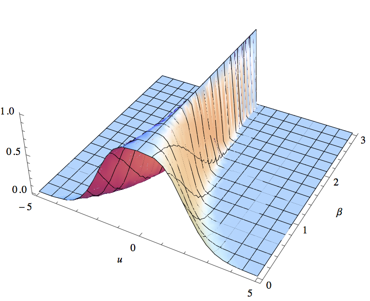
and for every parameter β≥0\beta\geq 0, the functions

u↦λ+​(u,β)2​cosh⁡β​e−e2​β​u22andu↦λ−​(u,β)2​cosh⁡β​e−e2​β​u22u\mapsto\frac{\lambda_{+}(u,\beta)}{2\cosh\beta}\,\mathrm{e}^{-\frac{\mathrm{e}^{2\beta}u^{2}}{2}}\quad\text{and}\quad u\mapsto\frac{\lambda_{-}(u,\beta)}{2\cosh\beta}\,\mathrm{e}^{-\frac{\mathrm{e}^{2\beta}u^{2}}{2}}

attain their unique maximum at u=0u=0, see Figure 3 for the graph of the first function.
Refer to caption
Figure 3. The function f⁡(u,β)=λ+​(u,β)2​cosh⁡β​e−e2​β​u22f(u,\beta)=\frac{\lambda_{+}(u,\beta)}{2\cosh\beta}\,\mathrm{e}^{-\frac{\mathrm{e}^{2\beta}u^{2}}{2}} (using Mathematica).

Their Taylor expansions at u=0u=0 are respectively

1−3​e6​β−e2​β24​u4+o⁡(u4)andtanh⁡β+o⁡(1),1-\frac{3\mathrm{e}^{6\beta}-\mathrm{e}^{2\beta}}{24}\,u^{4}+o(u^{4})\quad\text{and}\quad\tanh\beta+o(1),

so again by the Laplace method we get limn→∞∫ℝψn​(t)​𝑑t=∫ℝψ⁡(t)​𝑑t\lim_{n\to\infty}\int_{\mathbb{R}}\psi_{n}(t)\,dt=\int_{\mathbb{R}}\psi(t)\,dt and the L1\mathrm{L}^{1}-mod-convergence. As a consequence, consider the random configuration of spins σ\sigma on [[1,n]]\left[\!\left[1,n\right]\!\right] with probability proportional to

exp⁡(β⁡(∑i=1n−1σ⁡(i)​σ​(i+1))+12​n​e2​β​(∑i=1nσ⁡(i))2).\exp\left(\beta\left(\sum_{i=1}^{n-1}\sigma(i)\sigma(i+1)\right)+\frac{1}{2n\mathrm{e}^{2\beta}}\left(\sum_{i=1}^{n}\sigma(i)\right)^{2}\right).

This model has a local interaction with coefficient β\beta and a global interaction with coefficient 1e2​β\frac{1}{\mathrm{e}^{2\beta}}, so it is a mix of the Ising model and of the Curie-Weiss model. The previous discussion and Theorem 6 show that its magnetization satisfies the non standard limit theorem

Mnn3/4⇀n→∞ψ⁡(x)​d​x∫ℝψ⁡(x)​𝑑xwith ψ(x)=exp(−3​e6​β−e2​β24x4).\frac{M_{n}}{n^{3/4}}\rightharpoonup_{n\to\infty}\frac{\psi(x)\,dx}{\int_{\mathbb{R}}\psi(x)\,dx}\quad\text{with }\psi(x)=\exp\left(-\frac{3\mathrm{e}^{6\beta}-\mathrm{e}^{2\beta}}{24}\,x^{4}\right).

3.5. Sub-critical changes of measures

In the mixed Curie-Weiss-Ising model, one may ask what happens if instead of β\beta and 1e2​β\frac{1}{\mathrm{e}^{2\beta}} one puts arbitrary coefficients for the local and the global interaction. More generally, given a sequence (Xn)n∈ℕ(X_{n})_{n\in\mathbb{N}} that converges in the L1\mathrm{L}^{1}-mod-Gaussian sense with parameters tnt_{n} and limiting function ψ\psi, one can look at the change of measure

ℚn(γ)​[d​x]=eγ​x22​tn𝔼⁡[eγ​(Xn)22​tn]​ℙn​[d​x]\mathbb{Q}_{n}^{(\gamma)}[dx]=\frac{\mathrm{e}^{\frac{\gamma x^{2}}{2t_{n}}}}{\mathbb{E}\!\left[\mathrm{e}^{\frac{\gamma(X_{n})^{2}}{2t_{n}}}\right]}\,\mathbb{P}_{n}[dx]

with γ∈(0,1)\gamma\in(0,1) (for γ>1\gamma>1, the change of measure is not necessarily well-defined, since the hypotheses (A) and (B) do not ensure that 𝔼⁡[eγ​(Xn)2/2​tn]<+∞\mathbb{E}[\mathrm{e}^{\gamma(X_{n})^{2}/2t_{n}}]<+\infty). These subcritical changes of measures do not modify the order of magnitude of the fluctuations of XnX_{n}, and more precisely:

Theorem 10.

Suppose that (Xn)n∈ℕ(X_{n})_{n\in\mathbb{N}} converges in the L1\mathrm{L}^{1}-mod-Gaussian sense with parameters tnt_{n} and limiting function ψ\psi. Then, if (Xn(γ))n∈ℕ(X_{n}^{(\gamma)})_{n\in\mathbb{N}} is a sequence of random variables under the new probability measures ℚn(γ)\mathbb{Q}_{n}^{(\gamma)}, it converges in the L1\mathrm{L}^{1}-mod-Gaussian sense with parameters (1−γ)​tn(1-\gamma)t_{n} and limit ψ\psi.

Example.

Consider a random configuration of spins σ\sigma on [[1,n]]\left[\!\left[1,n\right]\!\right] with probability proportional to

exp⁡(β⁡(∑i=1n−1σ⁡(i)​σ​(i+1))+γ2​n​(∑i=1nσ⁡(i))2),\exp\left(\beta\left(\sum_{i=1}^{n-1}\sigma(i)\sigma(i+1)\right)+\frac{\gamma}{2n}\left(\sum_{i=1}^{n}\sigma(i)\right)^{2}\right),

with γ<e−2​β\gamma<\mathrm{e}^{-2\beta}. The total magnetization of the system has order of magnitude n1/2n^{1/2}, and more precisely, one has the central limit theorem

Mnn1/2⇀n→∞𝒩(0,(1−γe2​β)e2​β),\frac{M_{n}}{n^{1/2}}\rightharpoonup_{n\to\infty}\mathcal{N}(0,(1-\gamma\mathrm{e}^{2\beta})\mathrm{e}^{2\beta}),

and in fact a L1\mathrm{L}^{1}-mod-Gaussian convergence of Mnn1/4\frac{M_{n}}{n^{1/4}}, with a limiting function

ψ(x)=exp(−(3e6​β−e2​β)x4/24)\psi(x)=\exp(-(3\mathrm{e}^{6\beta}-\mathrm{e}^{2\beta})\,x^{4}/24)

that does not depend on γ\gamma.

Proof of Theorem 10.

We denote as before (Yn)n∈ℕ(Y_{n})_{n\in\mathbb{N}} a sequence of random variables under the laws ℚn=ℚn(1)\mathbb{Q}_{n}=\mathbb{Q}_{n}^{(1)}. We first compute the asymptotics of Zn(γ)=𝔼⁡[eγ​(Xn)2/2​tn]Z_{n}^{(\gamma)}=\mathbb{E}[\mathrm{e}^{\gamma(X_{n})^{2}/2t_{n}}]:

Zn(γ)\displaystyle Z_{n}^{(\gamma)} =Zn𝔼[e−(1−γ)(Yn)2/2tn]\displaystyle=Z_{n}\,\,\mathbb{E}[\mathrm{e}^{-(1-\gamma)(Y_{n})^{2}/2t_{n}}]
=tn2​π​(∫ℝψ⁡(x)​𝑑x)​𝔼​[e−tn​(1−γ)2​(Yntn)2]​(1+o⁡(1))\displaystyle=\sqrt{\frac{t_{n}}{2\pi}}\left(\int_{\mathbb{R}}\psi(x)\,dx\right)\,\mathbb{E}\!\left[\mathrm{e}^{-\frac{t_{n}(1-\gamma)}{2}(\frac{Y_{n}}{t_{n}})^{2}}\right](1+o(1))
=tn2​π​(∫ℝψ⁡(x)​𝑑x)​𝔼​[e−tn​(1−γ)2​(Wn)2]​(1+o⁡(1))\displaystyle=\sqrt{\frac{t_{n}}{2\pi}}\left(\int_{\mathbb{R}}\psi(x)\,dx\right)\,\mathbb{E}\!\left[\mathrm{e}^{-\frac{t_{n}(1-\gamma)}{2}\,(W_{n})^{2}}\right](1+o(1))
=11−γ​(1+o​(1))\displaystyle=\sqrt{\frac{1}{1-\gamma}}\,(1+o(1))

by using on the third line the same argument as in the proof of Proposition 7 to replace Yntn\frac{Y_{n}}{t_{n}} by WnW_{n}; and by using the Laplace method on the fourth line in order to compute ∫ℝe−tn(1−γ)x2/2ψn(x)dx\int_{\mathbb{R}}\mathrm{e}^{-t_{n}(1-\gamma)x^{2}/2}\,\psi_{n}(x)\,dx. The same computations give the asymptotics of

𝔼⁡[et​Xn+γ​(Xn)2/2​tn]\displaystyle\mathbb{E}[\mathrm{e}^{tX_{n}+\gamma(X_{n})^{2}/2t_{n}}] =Zn​𝔼​[et​Yn−(1−γ)​(Yn)2/2​tn]\displaystyle=Z_{n}\,\mathbb{E}[\mathrm{e}^{tY_{n}-(1-\gamma)(Y_{n})^{2}/2t_{n}}]
=tn2​π​(∫ℝψ⁡(x)​𝑑x)​𝔼​[etn​t​(Yntn)−tn​(1−γ)2​(Yntn)2]​(1+o⁡(1))\displaystyle=\sqrt{\frac{t_{n}}{2\pi}}\left(\int_{\mathbb{R}}\psi(x)\,dx\right)\,\mathbb{E}\!\left[\mathrm{e}^{t_{n}t\,(\frac{Y_{n}}{t_{n}})-\frac{t_{n}(1-\gamma)}{2}(\frac{Y_{n}}{t_{n}})^{2}}\right](1+o(1))
=tn2​π​(∫ℝψ⁡(x)​𝑑x)​𝔼​[etn​t​Wn−tn​(1−γ)2​(Wn)2]​(1+o⁡(1))\displaystyle=\sqrt{\frac{t_{n}}{2\pi}}\left(\int_{\mathbb{R}}\psi(x)\,dx\right)\,\mathbb{E}\!\left[\mathrm{e}^{t_{n}t\,W_{n}-\frac{t_{n}(1-\gamma)}{2}(W_{n})^{2}}\right](1+o(1))
=e−tn​t22​(1−γ)​11−γ​ψ​(t)​(1+o⁡(1))\displaystyle=\mathrm{e}^{-\frac{t_{n}t^{2}}{2(1-\gamma)}}\sqrt{\frac{1}{1-\gamma}}\,\psi(t)\,(1+o(1))

with again a Laplace method on the fourth line. Since

𝔼⁡[et​Xn(γ)]=𝔼⁡[et​Xn+γ​(Xn)2/2​tn]Zn(γ),\mathbb{E}[\mathrm{e}^{tX_{n}^{(\gamma)}}]=\frac{\mathbb{E}[\mathrm{e}^{tX_{n}+\gamma(X_{n})^{2}/2t_{n}}]}{Z_{n}^{(\gamma)}},

this shows the hypotheses (A) and (B) for the sequence (Xn(γ))n∈ℕ(X_{n}^{(\gamma)})_{n\in\mathbb{N}}. Then, since (Yntn)n∈ℕ(\frac{Y_{n}}{t_{n}})_{n\in\mathbb{N}} converges in law, by using the implication (ii) ⇒\Rightarrow (iii) in Theorem 6 for the sequence (Xn(γ))n∈ℕ(X_{n}^{(\gamma)})_{n\in\mathbb{N}}, we see that the mod-Gaussian convergence of Laplace transforms necessarily happens in L1​(ℝ)\mathrm{L}^{1}(\mathbb{R}). ∎

3.6. Random walks changed in measure

In this section, we shall make a brief excursion in the higher dimensions. Since we do not want to enter details on mod-Gaussian convergence for random vectors (for which we refer the reader to [KN12] and [FMN13]), we shall only consider the simple case X=(X(1),…,X(d))X=(X^{(1)},\ldots,X^{(d)}) is a random vector with values in ℝd\mathbb{R}^{d} such that 𝔼⁡[exp⁡(z1​X(1)+⋯+zd​X(d))]\mathbb{E}[\exp(z_{1}X^{(1)}+\cdots+z_{d}X^{(d)})] is entire in ℂd\mathbb{C}^{d}. We shall say that the sequence (Xn)(X_{n}) of random vectors converges in the complex mod-Gaussian sense with parameter tnt_{n} and limiting function ψ⁡(z1,⋯,zd)\psi(z_{1},\cdots,z_{d}) if the following convergence holds locally uniformly on compact subsets of ℂd\mathbb{C}^{d}:

ψn​(t)=𝔼⁡[exp⁡(z1​Xn(1)+⋯+zd​Xn(d))]​exp⁡(−tn​(z1)2+⋯+(zd)22)→ψ⁡(z1,…,zd).\psi_{n}(t)=\mathbb{E}[\exp(z_{1}X_{n}^{(1)}+\cdots+z_{d}X_{n}^{(d)})]\exp\left(-t_{n}\frac{(z_{1})^{2}+\cdots+(z_{d})^{2}}{2}\right)\to\psi(z_{1},\ldots,z_{d}).

In this vector setting, the assumptions (A) and (B) of Section 3 now simply amount to the fact that the convergence above holds locally uniformly for t=(t(1),⋯,t(d))∈ℝdt=(t^{(1)},\cdots,t^{(d)})\in\mathbb{R}^{d} and that ψn\psi_{n} and ψ\psi are both in L1​(ℝd)\mathrm{L}^{1}(\mathbb{R}^{d}).

Following the case d=1d=1 we denote ℙn\mathbb{P}_{n} the law of XnX_{n} on ℝd\mathbb{R}^{d},

ℚn​[d​x]=e‖x‖22​tn𝔼⁡[e‖Xn‖22​tn]​ℙn​[d​x],\mathbb{Q}_{n}[dx]=\frac{\mathrm{e}^{\frac{\|x\|^{2}}{2t_{n}}}}{\mathbb{E}\!\left[\mathrm{e}^{\frac{\|X_{n}\|^{2}}{2t_{n}}}\right]}\,\,\mathbb{P}_{n}[dx],

and YnY_{n} a random variable under the new law ℚn\mathbb{Q}_{n}. Note that here again hypothesis (B) implies that Zn=𝔼⁡[e‖Xn‖2/2​tn]Z_{n}=\mathbb{E}[\mathrm{e}^{\|X_{n}\|^{2}/2t_{n}}] is finite for all n∈ℕn\in\mathbb{N}. Indeed, with the notation ⟨u,v⟩=u1​v1+⋯+ud​vd\langle u,v\rangle=u_{1}v_{1}+\cdots+u_{d}v_{d}, we have

∫ℝdψn​(t)​𝑑t\displaystyle\int_{\mathbb{R}^{d}}\psi_{n}(t)\,dt =𝔼⁡[∫ℝde⟨t,Xn⟩−tn​‖t‖22​𝑑t]\displaystyle=\mathbb{E}\!\left[\int_{\mathbb{R}^{d}}\mathrm{e}^{\langle t,X_{n}\rangle-\frac{t_{n}\,\|t\|^{2}}{2}}\,dt\right]
=𝔼⁡[e(‖Xn‖2CLOSE2​tn​(∫ℝde−‖Xn−tn​t‖22​tn​𝑑t)]=(2​πtn)d/2​𝔼​[e‖Xn‖22​tn].\displaystyle=\mathbb{E}\!\left[\mathrm{e}^{\frac{(\|X_{n}\|^{2}}{2t_{n}}}\,\left(\int_{\mathbb{R}^{d}}\mathrm{e}^{-\frac{\|X_{n}-t_{n}t\|^{2}}{2t_{n}}}\,dt\right)\right]=\left(\frac{2\pi}{t_{n}}\right)^{d/2}\,\,\mathbb{E}\!\left[\mathrm{e}^{\frac{\|X_{n}\|^{2}}{2t_{n}}}\right].

Therefore, the new probabilities ℚn\mathbb{Q}_{n} are well-defined and

Zn=𝔼⁡[e‖Xn‖2/2​tn]=(tn2​π)d/2​∫ℝdψn​(t)​𝑑t.Z_{n}=\mathbb{E}[\mathrm{e}^{\|X_{n}\|^{2}/2t_{n}}]=\left(\frac{t_{n}}{2\pi}\right)^{d/2}\int_{\mathbb{R}^{d}}\psi_{n}(t)\,dt.

Then it is clear that Proposition 5 holds with GnG_{n} being a Gaussian vector with covariance matrix 1/tn​Id1/t_{n}\;I_{d} where IdI_{d} is the identity matrix of size dd. Similarly one can establish an analogue of Theorem 6 in ℝd\mathbb{R}^{d}.

Let WnW_{n} be a simple random walk on the lattice ℤd≥2\mathbb{Z}^{d\geq 2}: at each step, each of the 2​d2d neighbors of the state that is occupied has the same probability of transition (2​d)−1(2d)^{-1}. The dd-dimensional characteristic function of Wn=(Wn(1),…,Wn(d))W_{n}=(W_{n}^{(1)},\ldots,W_{n}^{(d)}) is

𝔼⁡[ez1​Wn(1)+⋯+zd​Wn(d)]=(cosh⁡z1+⋯+cosh⁡zdd)n.\mathbb{E}[\mathrm{e}^{z_{1}W_{n}^{(1)}+\cdots+z_{d}W_{n}^{(d)}}]=\left(\frac{\cosh z_{1}+\cdots+\cosh z_{d}}{d}\right)^{n}.

Therefore, one has the asymptotics

log⁡𝔼⁡[ez1​Wn(1)+⋯+zd​Wn(d)n1/4]\displaystyle\log\,\mathbb{E}\!\left[\mathrm{e}^{\frac{z_{1}W_{n}^{(1)}+\cdots+z_{d}W_{n}^{(d)}}{n^{1/4}}}\right]
=n​log⁡(1+(z1)2+⋯+(zd)22​d​n1/2+(z1)4+⋯+(zd)424​d​n+o⁡(1n))\displaystyle=n\log\left(1+\frac{(z_{1})^{2}+\cdots+(z_{d})^{2}}{2dn^{1/2}}+\frac{(z_{1})^{4}+\cdots+(z_{d})^{4}}{24dn}+o\left(\frac{1}{n}\right)\right)
=n1/2​(z1)2+⋯+(zd)22​d−3​((z1)2+⋯+(zd)2)2−d⁡((z1)4+⋯+(zd)4)24​d2+o⁡(1).\displaystyle=n^{1/2}\,\frac{(z_{1})^{2}+\cdots+(z_{d})^{2}}{2d}-\frac{3((z_{1})^{2}+\cdots+(z_{d})^{2})^{2}-d((z_{1})^{4}+\cdots+(z_{d})^{4})}{24d^{2}}+o(1).

One obtains a dd-dimensional complex mod-Gaussian convergence of Xn=n−1/4WnX_{n}=n^{-1/4}\,W_{n} with parameters n1/2d\frac{n^{1/2}}{d} and limiting function

ψ⁡(z1,…,zd)=exp⁡(−3​((z1)2+⋯+(zd)2)2−d⁡((z1)4+⋯+(zd)4)24​d2).\psi(z_{1},\ldots,z_{d})=\exp\left(-\frac{3\,((z_{1})^{2}+\cdots+(z_{d})^{2})^{2}-d\,((z_{1})^{4}+\cdots+(z_{d})^{4})}{24d^{2}}\right).

In [FMN13], we used this mod-convergence to prove quantitative estimates regarding the breaking of the radial symmetry when one considers random walks conditioned to be of large size (of order n3/4n^{3/4} instead of the expected order n1/2n^{1/2}). With the notion of L1\mathrm{L}^{1}-mod-Gaussian convergence, one can give another interpretation, but only for d=2d=2 or d=3d=3. Restricted to ℝd\mathbb{R}^{d}, the limiting function is indeed not integrable for d≥4d\geq 4: if t2,…,td∈[−1,1]t_{2},\ldots,t_{d}\in[-1,1], then

3​((t1)2+⋯+(td)2)2−d\displaystyle 3\,((t_{1})^{2}+\cdots+(t_{d})^{2})^{2}-d\, ((t1)4+⋯+(td)4)≤3​((t1)2+(d−1))2−d​(t1)4\displaystyle((t_{1})^{4}+\cdots+(t_{d})^{4})\leq 3\,((t_{1})^{2}+(d-1))^{2}-d\,(t_{1})^{4}
≤(3−d)​(t1)4+6​(d−1)​(t1)2+3​(d−1)2.\displaystyle\leq(3-d)(t_{1})^{4}+6(d-1)(t_{1})^{2}+3(d-1)^{2}.

So, restricted to the domain ℝ×[−1,1]d−1\mathbb{R}\times[-1,1]^{d-1}, ψ⁡(t1,…,td)≤K​exp⁡(a​(t1)4−b​(t1)2)\psi(t_{1},\ldots,t_{d})\leq K\,\exp(a(t_{1})^{4}-b(t_{1})^{2}) for some positive constants aa, bb and KK; therefore, this function is not integrable.

On the other hand, if d=2d=2 or d=3d=3, then ψ\psi is integrable on ℝd\mathbb{R}^{d}, and one has L1\mathrm{L}^{1}-mod-Gaussian convergence. Indeed, when d=2d=2, the limiting function is

(10) ψ⁡(t1,t2)=exp⁡(−(t1)4+(t2)4+6​(t1​t2)296),\psi(t_{1},t_{2})=\exp\left(-\frac{(t_{1})^{4}+(t_{2})^{4}+6(t_{1}t_{2})^{2}}{96}\right),

which is clearly integrable; and the residues

ψn​(t1,t2)=𝔼⁡[et1​Wn(1)+t2​Wn(2)n1/4]​e−n1/2​((t1)2+(t2)2)4\psi_{n}(t_{1},t_{2})=\mathbb{E}\left[\mathrm{e}^{\frac{t_{1}W_{n}^{(1)}+t_{2}W_{n}^{(2)}}{n^{1/4}}}\right]\,\mathrm{e}^{-\frac{n^{1/2}((t_{1})^{2}+(t_{2})^{2})}{4}}

converge locally uniformly on ℝ2\mathbb{R}^{2} to ψ⁡(t1,t2)\psi(t_{1},t_{2}), but also in L1​(ℝ2)\mathrm{L}^{1}(\mathbb{R}^{2}). Indeed,

∫ℝ2ψn​(t1,t2)​d​t1​d​t2\displaystyle\int_{\mathbb{R}^{2}}\psi_{n}(t_{1},t_{2})\,dt_{1}\,dt_{2} =∫ℝ2(cosh⁡t1n1/4+cosh⁡t2n1/42)n​e−n1/2​((t1)2+(t2)2)4​d​t1​d​t2\displaystyle=\int_{\mathbb{R}^{2}}\left(\frac{\cosh\frac{t_{1}}{n^{1/4}}+\cosh\frac{t_{2}}{n^{1/4}}}{2}\right)^{n}\mathrm{e}^{-\frac{n^{1/2}((t_{1})^{2}+(t_{2})^{2})}{4}}\,dt_{1}\,dt_{2}
=n1/2​∫ℝ2(cosh⁡u1+cosh⁡u22​e−(u1)2+(u2)24)n​d​u1​d​u2,\displaystyle=n^{1/2}\int_{\mathbb{R}^{2}}\left(\frac{\cosh u_{1}+\cosh u_{2}}{2}\,\mathrm{e}^{-\frac{(u_{1})^{2}+(u_{2})^{2}}{4}}\right)^{n}\,du_{1}\,du_{2},

and the function (u1,u2)↦cosh⁡u1+cosh⁡u22​e−(u1)2+(u2)24(u_{1},u_{2})\mapsto\frac{\cosh u_{1}+\cosh u_{2}}{2}\,\mathrm{e}^{-\frac{(u_{1})^{2}+(u_{2})^{2}}{4}} reaches its unique global maximum at u1=u2=0u_{1}=u_{2}=0, with Taylor expansion

1−(u1)4+(u2)4+6​(u1​u2)296+o⁡(‖u‖4)1-\frac{(u_{1})^{4}+(u_{2})^{4}+6(u_{1}u_{2})^{2}}{96}+o(\|u\|^{4})

around this point (see Figure 4).

Refer to caption
Figure 4. The function f⁡(u1,u2)=cosh⁡u1+cosh⁡u22​e−(u1)2+(u2)24f(u_{1},u_{2})=\frac{\cosh u_{1}+\cosh u_{2}}{2}\,\mathrm{e}^{-\frac{(u_{1})^{2}+(u_{2})^{2}}{4}}.

Thus, by using the multi-dimensional Laplace method, one sees that the limit of the integral ∫ℝ2ψn​(t1,t2)​d​t1​d​t2\int_{\mathbb{R}^{2}}\psi_{n}(t_{1},t_{2})\,dt_{1}\,dt_{2} is ∫ℝ2ψ⁡(t1,t2)​d​t1​d​t2\int_{\mathbb{R}^{2}}\psi(t_{1},t_{2})\,dt_{1}\,dt_{2}, and the L1\mathrm{L}^{1} convergence is shown. Similarly, when d=3d=3, the limiting function is

(11) ψ⁡(t1,t2,t3)=exp⁡(−(t1​t2)2+(t1​t3)2+(t2​t3)236),\psi(t_{1},t_{2},t_{3})=\exp\left(-\frac{(t_{1}t_{2})^{2}+(t_{1}t_{3})^{2}+(t_{2}t_{3})^{2}}{36}\right),

and the following computation shows that it is integrable:

∫ℝ3ψ⁡(x,y,z)​𝑑x​𝑑y​𝑑z\displaystyle\int_{\mathbb{R}^{3}}\psi(x,y,z)\,dx\,dy\,dz =∫ℝ2e−(y​z)236​(∫ℝe−y2+z236​x2​𝑑x)​𝑑y​𝑑z\displaystyle=\int_{\mathbb{R}^{2}}\mathrm{e}^{-\frac{(yz)^{2}}{36}}\left(\int_{\mathbb{R}}\mathrm{e}^{-\frac{y^{2}+z^{2}}{36}\,x^{2}}dx\right)dy\,dz
=6​π​∫ℝ2e−(y​z)236y2+z2​𝑑y​𝑑z\displaystyle=6\sqrt{\pi}\int_{\mathbb{R}^{2}}\frac{\mathrm{e}^{-\frac{(yz)^{2}}{36}}}{\sqrt{y^{2}+z^{2}}}\,dy\,dz
=3​π​∫r=0∞∫θ=0πe−r4​sin2⁡θ144​𝑑r​𝑑θ\displaystyle=3\sqrt{\pi}\int_{r=0}^{\infty}\int_{\theta=0}^{\pi}\mathrm{e}^{-\frac{r^{4}\,\sin^{2}\theta}{144}}\,dr\,d\theta
=12​3​π​∫r=0∞e−r4​𝑑r​∫θ=0π2d​θsin⁡θ<+∞\displaystyle=12\sqrt{3\pi}\int_{r=0}^{\infty}\mathrm{e}^{-r^{4}}\,dr\int_{\theta=0}^{\frac{\pi}{2}}\frac{d\theta}{\sqrt{\sin\theta}}<+\infty

since 1sin⁡θ\frac{1}{\sqrt{\sin\theta}} is integrable at 00. On the other hand, the residues

ψn​(t1,t2,t3)=𝔼⁡[et1​Wn(1)+t2​Wn(2)+t3​Wn(3)n1/4]​e−n1/2​((t1)2+(t2)2+(t3)2)6\psi_{n}(t_{1},t_{2},t_{3})=\mathbb{E}\left[\mathrm{e}^{\frac{t_{1}W_{n}^{(1)}+t_{2}W_{n}^{(2)}+t_{3}W_{n}^{(3)}}{n^{1/4}}}\right]\,\mathrm{e}^{-\frac{n^{1/2}((t_{1})^{2}+(t_{2})^{2}+(t_{3})^{2})}{6}}

converge to ψ⁡(t1,t2,t3)\psi(t_{1},t_{2},t_{3}) locally uniformly on ℝ3\mathbb{R}^{3} and in L1​(ℝ3)\mathrm{L}^{1}(\mathbb{R}^{3}). Indeed, one has again

∫ℝ3ψn​(t1,t2,t3)​𝑑t=n1/2​∫ℝ3(cosh⁡u1+cosh⁡u2+cosh⁡u33​e−(u1)2+(u2)2+(u3)26)n​𝑑u\int_{\mathbb{R}^{3}}\psi_{n}(t_{1},t_{2},t_{3})\,dt=n^{1/2}\int_{\mathbb{R}^{3}}\left(\frac{\cosh u_{1}+\cosh u_{2}+\cosh u_{3}}{3}\,\mathrm{e}^{-\frac{(u_{1})^{2}+(u_{2})^{2}+(u_{3})^{2}}{6}}\right)^{n}\,du

and the function in the brackets reaches its unique maximum at u1=u2=u3=0u_{1}=u_{2}=u_{3}=0, with Taylor expansion corresponding to the limiting function ψ\psi after application of the Laplace method.

The multidimensional analogue of Theorem 6 thus yields the following multidimensional extension of the limit theorem for the Curie-Weiss model:

Theorem 11.

Let WnW_{n} be a simple random walk in dimension d≤3d\leq 3. If VnV_{n} is obtained from WnW_{n} by a change of measure by the factor exp⁡(d​‖Wn‖2/2​n)\exp(d\,\|W_{n}\|^{2}/2n), then

Vnn3/4⇀n→∞ψ⁡(x)​d​x∫ℝ3ψ⁡(x)​𝑑x,\frac{V_{n}}{n^{3/4}}\rightharpoonup_{n\to\infty}\frac{\psi(x)\,dx}{\int_{\mathbb{R}^{3}}\psi(x)\,dx},

where ψ(x)=exp(−x4/12)\psi(x)=\exp(-x^{4}/12) in dimension 11, and ψ\psi is given by Formulas (10) and (11) in dimension 22 and 33.

Remark.

Suppose d=2d=2. Then, there is a limit in law not only for Vnn3/4\frac{V_{n}}{n^{3/4}}, but in fact for the whole random walk (Vkn3/4)k≤n(\frac{V_{k}}{n^{3/4}})_{k\leq n}, viewed as a random element of 𝒞⁡(ℝ+,ℝ2)\mathcal{C}(\mathbb{R}_{+},\mathbb{R}^{2}) or of the Skorohod space 𝒟⁡(ℝ+,ℝ2)\mathcal{D}(\mathbb{R}_{+},\mathbb{R}^{2}), see Figure 5.

Figure 5. A 22-dimensional random walk changed in measure by e‖Wn‖2/n\mathrm{e}^{\|W_{n}\|^{2}/n}, here with n=10000n=10000.

4. Local limit theorem and rate of convergence in the Ellis-Newman limit theorem

We keep the same notation as before and note In=∫ℝψn​(x)​𝑑xI_{n}=\int_{\mathbb{R}}\psi_{n}(x)\,dx and I∞=∫ℝψ⁡(x)​𝑑xI_{\infty}=\int_{\mathbb{R}}\psi(x)\,dx. In this section we wish to provide a quick approach based on Fourier analysis,

  1. (1)

    to compute the Kolmogorov distance between the rescaled magnetization

    Yn/n1/2=Mn/n3/4Y_{n}/n^{1/2}=M_{n}/n^{3/4}

    in the Curie-Weiss model and the random variable W∞W_{\infty} with density ψ⁡(x)/I∞\psi(x)/I_{\infty}, where ψ(x)=exp(−x4/12)\psi(x)=\exp(-x^{4}/12). This problem was recently solved in [EL10] using Stein’s method. As in [EL10], our method would cover many more general models as well: it is just a matter of specializing Lemma 12 and Lemma 13 below which are stated in all generality.

  2. (2)

    to prove a new local limit theorem for the rescaled magnetization n−1/4Mnn^{-1/4}M_{n} in the Curie-Weiss model. Here again we shall indicate how one can establish local limit theorems in more general situations.

4.1. Speed of convergence

Getting back to our special case of the Curie-Weiss model, we denote Xn=1n1/4​∑i=1nBiX_{n}=\frac{1}{n^{1/4}}\sum_{i=1}^{n}B_{i} a scaled sum of ±1\pm 1 independent Bernoulli random variables; YnY_{n} the random variable with modified law

ℚn​[d​y]=ey22​n1/2​ℙn​[d​y]𝔼⁡[e(Xn)22​n1/2];\mathbb{Q}_{n}[dy]=\frac{\mathrm{e}^{\frac{y^{2}}{2n^{1/2}}}\,\mathbb{P}_{n}[dy]}{\mathbb{E}\!\left[\mathrm{e}^{\frac{(X_{n})^{2}}{2n^{1/2}}}\right]};

GnG_{n} an independent Gaussian random variable of variance 1n1/2\frac{1}{n^{1/2}}; and Wn=Ynn1/2+GnW_{n}=\frac{Y_{n}}{n^{1/2}}+G_{n}. It follows from the previous results that the law of WnW_{n} has density

ψn​(x)In=1In​e−n1/2​x22​(cosh⁡xn1/4)n,\frac{\psi_{n}(x)}{I_{n}}=\frac{1}{I_{n}}\,\mathrm{e}^{-\frac{n^{1/2}x^{2}}{2}}\,\left(\cosh\frac{x}{n^{1/4}}\right)^{n},

which converges in L1\mathrm{L}^{1} towards the law ψ⁡(x)I∞=1I∞​e−x412\frac{\psi(x)}{I_{\infty}}=\frac{1}{I_{\infty}}\,\mathrm{e}^{-\frac{x^{4}}{12}}. We hence wish for an upper bound for the Kolmogorov distance between Ynn1/2\frac{Y_{n}}{n^{1/2}} and W∞W_{\infty}. For this we shall need the following general lemmas.

Lemma 12.

Consider the two distributions Wn=ψn​(x)​d​xInW_{n}=\frac{\psi_{n}(x)\,dx}{I_{n}} and W∞=ψ⁡(x)​d​xI∞W_{\infty}=\frac{\psi(x)\,dx}{I_{\infty}}. The Kolmogorov distance between them is smaller than

‖ψ−ψn‖L1I∞​(1+o​(1)).\frac{\|\psi-\psi_{n}\|_{\mathrm{L}^{1}}}{I_{\infty}}\,(1+o(1)).
Proof.

Fix a∈ℝa\in\mathbb{R}, and suppose for instance that ∫ℝψ⁡(x)​𝑑x≥∫ℝψn​(x)​𝑑x\int_{\mathbb{R}}\psi(x)\,dx\geq\int_{\mathbb{R}}\psi_{n}(x)\,dx. We have

FWn​(a)−FW∞​(a)\displaystyle F_{W_{n}}(a)-F_{W_{\infty}}(a) =(∫−∞aψn​(x)​𝑑xIn−∫−∞aψ⁡(x)​𝑑xIn)+(∫−∞aψ⁡(x)​𝑑xIn−∫−∞aψ⁡(x)​𝑑xI∞)\displaystyle=\left(\frac{\int_{-\infty}^{a}\psi_{n}(x)\,dx}{I_{n}}-\frac{\int_{-\infty}^{a}\psi(x)\,dx}{I_{n}}\right)\!+\!\left(\frac{\int_{-\infty}^{a}\psi(x)\,dx}{I_{n}}-\frac{\int_{-\infty}^{a}\psi(x)\,dx}{I_{\infty}}\right)
=∫−∞a(ψn​(x)−ψ⁡(x))​𝑑xIn+(∫−∞aψ⁡(x)​𝑑x)​∫−∞∞(ψ⁡(x)−ψn​(x))​𝑑xI∞​In\displaystyle=\frac{\int_{-\infty}^{a}(\psi_{n}(x)-\psi(x))\,dx}{I_{n}}+\left(\int_{-\infty}^{a}\psi(x)\,dx\right)\frac{\int_{-\infty}^{\infty}(\psi(x)-\psi_{n}(x))\,dx}{I_{\infty}I_{n}}
≤−∫−∞a(ψ⁡(x)−ψn​(x))​𝑑xIn+∫−∞∞(ψ⁡(x)−ψn​(x))​𝑑xIn\displaystyle\leq-\frac{\int_{-\infty}^{a}(\psi(x)-\psi_{n}(x))\,dx}{I_{n}}+\frac{\int_{-\infty}^{\infty}(\psi(x)-\psi_{n}(x))\,dx}{I_{n}}
≤∫a∞(ψ⁡(x)−ψn​(x))​𝑑xIn≤‖ψ−ψn‖L1In.\displaystyle\leq\frac{\int_{a}^{\infty}(\psi(x)-\psi_{n}(x))\,dx}{I_{n}}\leq\frac{\|\psi-\psi_{n}\|_{\mathrm{L}^{1}}}{I_{n}}.

Writing FW∞​(a)−FWn​(a)=(1−FWn​(a))−(1−FW∞​(a))F_{W_{\infty}}(a)-F_{W_{n}}(a)=(1-F_{W_{n}}(a))-(1-F_{W_{\infty}}(a)), one sees that the inequality is in fact valid with an absolute value on the left-hand side. Since In=I∞​(1+o⁡(1))I_{n}=I_{\infty}(1+o(1)), this shows the claim. If ∫ℝψn​(x)​𝑑x≥∫ℝψ⁡(x)​𝑑x\int_{\mathbb{R}}\psi_{n}(x)\,dx\geq\int_{\mathbb{R}}\psi(x)\,dx, it suffices to exchange the roles played by ψn\psi_{n} and ψ\psi to get the inequality. ∎

The asymptotics of the L1\mathrm{L}^{1}-norm ‖ψ−ψn‖L1\|\psi-\psi_{n}\|_{\mathrm{L}^{1}} in the Curie-Weiss model are computed as follows. Noting that one always has ψn​(x)≥ψ⁡(x)\psi_{n}(x)\geq\psi(x), it suffices to compute

∫ℝψn(x)dx=∫ℝe−n1/2​x22(cosh(xn−1/4))ndx=n1/4∫ℝ(e−u22cosh(u))ndu.\int_{\mathbb{R}}\psi_{n}(x)\,dx=\int_{\mathbb{R}}\mathrm{e}^{-\frac{n^{1/2}\,x^{2}}{2}}\,\left(\cosh(x\,n^{-1/4})\right)^{n}\,dx=n^{1/4}\int_{\mathbb{R}}\left(\mathrm{e}^{-\frac{u^{2}}{2}}\,\cosh(u)\right)^{n}\,du.

By the Laplace method (see [Zor04, Formula (19.17), p. 624-625]), the asymptotics of the integral is

n−14​(121/4​Γ​(14)2)+n−34​(123/4​Γ​(34)10)+smaller terms.n^{-\frac{1}{4}}\left(\frac{{12}^{1/4}\,\Gamma(\frac{1}{4})}{2}\right)+n^{-\frac{3}{4}}\left(\frac{12^{3/4}\,\Gamma(\frac{3}{4})}{10}\right)+\text{smaller terms}.

The first term corresponds to I∞=∫ℝψ(x)dx=∫ℝe−x4/12dxI_{\infty}=\int_{\mathbb{R}}\psi(x)\,dx=\int_{\mathbb{R}}\mathrm{e}^{-x^{4}/12}\,dx. As a consequence,

‖ψ−ψn‖L1I∞=1n1/2​12​Γ​(34)5​Γ​(14)​(1+o⁡(1)).\frac{\|\psi-\psi_{n}\|_{\mathrm{L}^{1}}}{I_{\infty}}=\frac{1}{n^{1/2}}\,\frac{\sqrt{12}\,\Gamma(\frac{3}{4})}{5\,\Gamma(\frac{1}{4})}\,(1+o(1)).

The main work now consists in computing dKol​(Ynn1/2,Wn)d_{\mathrm{Kol}}(\frac{Y_{n}}{n^{1/2}},W_{n}). We start by a Lemma which is a variation of arguments used for i.i.d. random variables in [Tao12, p. 87]. In the following, given a function f∈L1​(ℝ)f\in\mathrm{L}^{1}(\mathbb{R}), we write its Fourier transform f^​(ξ)=∫ℝf⁡(x)​ei​ξ​x​𝑑x\widehat{f}(\xi)=\int_{\mathbb{R}}f(x)\,\mathrm{e}^{\mathrm{i}\xi x}\,dx. Recall that the function

υ⁡(ξ)={e−11−4​ξ2if ​|ξ|<12,0otherwise.\upsilon(\xi)=\begin{cases}\mathrm{e}^{-\frac{1}{1-4\xi^{2}}}&\text{if }|\xi|<\frac{1}{2},\\ 0&\text{otherwise}.\end{cases}

is even, of class 𝒞∞\mathcal{C}^{\infty} and with compact support [−12,12][-\frac{1}{2},\frac{1}{2}]. We set ρ⋆^=υ\widehat{\rho_{\star}}=\upsilon, so that

ρ⋆​(x)=12​π​∫−1212υ⁡(ξ)​e−i​x​ξ​𝑑ξ\rho_{\star}(x)=\frac{1}{2\pi}\int_{-\frac{1}{2}}^{\frac{1}{2}}\upsilon(\xi)\,\mathrm{e}^{-\mathrm{i}x\xi}\,d\xi

by the Fourier inversion theorem. By construction, the Fourier transform of ρ⋆\rho_{\star} has support equal to [−12,12][-\frac{1}{2},\frac{1}{2}]. Set now

ρ⁡(x)=(ρ⋆​(x))2∫ℝ(ρ∗​(y))2​𝑑y.\rho(x)=\frac{(\rho_{\star}(x))^{2}}{\int_{\mathbb{R}}(\rho_{*}(y))^{2}\,dy}.

By construction, ρ\rho is smooth, even, non-negative and with integral equal to 11. Moreover, ρ^\widehat{\rho} is up to a constant equal to ν∗ν⁡(ξ)\nu*\nu(\xi), so it has support included into [−1,1][-1,1]. The convolution of ρ\rho with characteristic functions of intervals will allow us to transform estimates on test functions into estimates on cumulative distribution functions. More precisely, for a∈ℝa\in\mathbb{R} and ε>0\varepsilon>0, set ρε​(x)=1ε​ρ​(xε)\rho_{\varepsilon}(x)=\frac{1}{\varepsilon}\,\rho(\frac{x}{\varepsilon}), and ϕa,ε​(x)=ϕε​(x−a)\phi_{a,\varepsilon}(x)=\phi_{\varepsilon}(x-a), where ϕε\phi_{\varepsilon} is the function 1(−∞,0]∗ρε1_{(-\infty,0]}*\rho_{\varepsilon}. One sees ϕa,ε\phi_{a,\varepsilon} as a smooth approximation of the characteristic function 1(−∞,a]1_{(-\infty,a]}.

For all a,εa,\varepsilon, ϕa,ε\phi_{a,\varepsilon} has Fourier transform compactly supported on [−1ε,1ε]\left[-\frac{1}{\varepsilon},\frac{1}{\varepsilon}\right]. Moreover, it has negative derivative, and decreases from 11 to 00. Later, we will use the identity

ϕε​(ε​x)=ϕ1​(x)=ϕ⁡(x).\phi_{\varepsilon}(\varepsilon x)=\phi_{1}(x)=\phi(x).

On the other hand, we have the following estimates for K>0K>0 (we used Sage for numerical computations):

|ρ∗​(K)|\displaystyle|\rho_{*}(K)| =12​π​K2​|∫−1212υ′′​(ξ)​e−i​K​ξ​𝑑ξ|≤12​π​K2​∫012|υ′′​(ξ)|​𝑑ξ=1.0166−K2;\displaystyle=\frac{1}{2\pi K^{2}}\left|\int_{-\frac{1}{2}}^{\frac{1}{2}}\upsilon^{\prime\prime}(\xi)\,\mathrm{e}^{-\mathrm{i}K\xi}\,d\xi\right|\leq\frac{1}{2\pi K^{2}}\int_{0}^{\frac{1}{2}}|\upsilon^{\prime\prime}(\xi)|\,d\xi=\frac{1.0166_{-}}{K^{2}};
∫ℝ(ρ∗​(y))2​𝑑y\displaystyle\int_{\mathbb{R}}(\rho_{*}(y))^{2}\,dy =12​π​∫012|υ⁡(ξ)|2​𝑑ξ=0.01059+.\displaystyle=\frac{1}{2\pi}\int_{0}^{\frac{1}{2}}|\upsilon(\xi)|^{2}\,d\xi=0.01059_{+}.

Therefore, for any K>0K>0,

ρ⁡(K)\displaystyle\rho(K) =ρ⁡(−K)=(ρ∗​(K))2∫ℝ(ρ∗​(y))2​𝑑y≤99K4;\displaystyle=\rho(-K)=\frac{(\rho_{*}(K))^{2}}{\int_{\mathbb{R}}(\rho_{*}(y))^{2}\,dy}\leq\frac{99}{K^{4}};
ϕ⁡(K)\displaystyle\phi(K) =1−ϕ⁡(−K)=∫0∞ρ⁡(K+y)​𝑑y≤33K3.\displaystyle=1-\phi(-K)=\int_{0}^{\infty}\rho(K+y)\,dy\leq\frac{33}{K^{3}}.
Lemma 13.

Let VV and WW be two random variables with cumulative distribution functions FVF_{V} and FWF_{W}. Assume that for some ε>0\varepsilon>0

|𝔼⁡[ϕa,ε​(V)]−𝔼⁡[ϕa,ε​(W)]|≤B​ε,|\mathbb{E}[\phi_{a,\varepsilon}(V)]-\mathbb{E}[\phi_{a,\varepsilon}(W)]|\leq B\varepsilon,

where the positive constant BB is independent of aa. We also suppose that WW has a density w.r.t. Lebesgue measure that is bounded by mm. Then,

supa∈ℝ|FV​(a)−FW​(a)|≤2​(B+10​m)​ε.\sup_{a\in\mathbb{R}}|F_{V}(a)-F_{W}(a)|\leq 2(B+10m)\,\varepsilon.
Proof.

Fix a positive constant KK, and denote δ=supa∈ℝ|FV​(a)−FW​(a)|\delta=\sup_{a\in\mathbb{R}}|F_{V}(a)-F_{W}(a)| the Kolmogorov distance between VV and WW. One has

FV​(a)=𝔼⁡[1V≤a]\displaystyle F_{V}(a)=\mathbb{E}[1_{V\leq a}] ≤𝔼⁡[ϕa+K​ε,ε​(V)]+𝔼⁡[(1−ϕa+K​ε,ε​(V))​ 1V≤a]\displaystyle\leq\mathbb{E}[\phi_{a+K\varepsilon,\varepsilon}(V)]+\mathbb{E}[(1-\phi_{a+K\varepsilon,\varepsilon}(V))\,1_{V\leq a}]
≤𝔼⁡[ϕa+K​ε,ε​(W)]+𝔼⁡[(1−ϕa+K​ε,ε​(V))​ 1V≤a]+B​ε.\displaystyle\leq\mathbb{E}[\phi_{a+K\varepsilon,\varepsilon}(W)]+\mathbb{E}[(1-\phi_{a+K\varepsilon,\varepsilon}(V))\,1_{V\leq a}]+B\varepsilon.

The second expectation writes as

𝔼[(1−\displaystyle\mathbb{E}[(1- ϕa+K​ε,ε(V)) 1V≤a]=∫ℝ(1−ϕa+K​ε,ε(x)) 1(−∞,a](x)fV(x)dx\displaystyle\phi_{a+K\varepsilon,\varepsilon}(V))\,1_{V\leq a}]=\int_{\mathbb{R}}(1-\phi_{a+K\varepsilon,\varepsilon}(x))\,1_{(-\infty,a]}(x)\,f_{V}(x)\,dx
=−∫ℝ((1−ϕa+K​ε,ε(x)) 1(−∞,a](x))′FV(x)dx\displaystyle=-\int_{\mathbb{R}}((1-\phi_{a+K\varepsilon,\varepsilon}(x))\,1_{(-\infty,a]}(x))^{\prime}\,F_{V}(x)\,dx
=∫ℝϕa+K​ε,ε′(x) 1(−∞,a](x)FV(x)dx+∫ℝ(1−ϕa+K​ε,ε(x)) 1a(x)FV(x)dx.\displaystyle=\int_{\mathbb{R}}\phi_{a+K\varepsilon,\varepsilon}^{\prime}(x)\,1_{(-\infty,a]}(x)\,F_{V}(x)\,dx+\int_{\mathbb{R}}(1-\phi_{a+K\varepsilon,\varepsilon}(x))\,1_{a}(x)\,F_{V}(x)\,dx.

For the first integral, since FV​(x)≥FW​(x)−δF_{V}(x)\geq F_{W}(x)-\delta and the derivative of ϕa+K​ε,ε\phi_{a+K\varepsilon,\varepsilon} is negative, an upper bound on I1I_{1} is

∫ℝϕa+K​ε,ε′(x) 1(−∞,a](x)FW(x)dx−δ∫ℝϕa+K​ε,ε′(x) 1V≤a(x)\displaystyle\int_{\mathbb{R}}\phi_{a+K\varepsilon,\varepsilon}^{\prime}(x)\,1_{(-\infty,a]}(x)\,F_{W}(x)\,dx-\delta\int_{\mathbb{R}}\phi_{a+K\varepsilon,\varepsilon}^{\prime}(x)\,1_{V\leq a}(x)
=∫ℝϕa+K​ε,ε′(x) 1(−∞,a](x)FW(x)dx+(1−ϕa+K​ε,ε(a))δ\displaystyle=\int_{\mathbb{R}}\phi_{a+K\varepsilon,\varepsilon}^{\prime}(x)\,1_{(-\infty,a]}(x)\,F_{W}(x)\,dx+(1-\phi_{a+K\varepsilon,\varepsilon}(a))\,\delta
=∫ℝϕa+K​ε,ε′(x) 1(−∞,a](x)FW(x)dx+(1−ϕ(−K))δ.\displaystyle=\int_{\mathbb{R}}\phi_{a+K\varepsilon,\varepsilon}^{\prime}(x)\,1_{(-\infty,a]}(x)\,F_{W}(x)\,dx+(1-\phi(-K))\,\delta.

As for the second integral, it is simply (1−ϕa+Kε,ε​(a))​FV​(a)(1-\phi_{a+K_{\varepsilon},\varepsilon}(a))F_{V}(a), and by writing FV​(a)≤FW​(a)+δF_{V}(a)\leq F_{W}(a)+\delta, one gets the upper bound on I2I_{2}

∫ℝ(1−ϕa+K​ε,ε​(x))​ 1a​(x)​FW​(x)​𝑑x+(1−ϕa+K​ε,ε​(a))​δ\displaystyle\int_{\mathbb{R}}(1-\phi_{a+K\varepsilon,\varepsilon}(x))\,1_{a}(x)\,F_{W}(x)\,dx+(1-\phi_{a+K\varepsilon,\varepsilon}(a))\,\delta
=∫ℝ(1−ϕa+K​ε,ε​(x))​ 1a​(x)​FW​(x)​𝑑x+(1−ϕ⁡(−K))​δ.\displaystyle=\int_{\mathbb{R}}(1-\phi_{a+K\varepsilon,\varepsilon}(x))\,1_{a}(x)\,F_{W}(x)\,dx+(1-\phi(-K))\,\delta.

One concludes that

𝔼⁡[(1−ϕa+K​ε,ε​(V))​ 1V≤a]≤𝔼⁡[(1−ϕa+K​ε,ε​(W))​ 1W≤a]+2​(1−ϕ⁡(−K))​δ.\mathbb{E}[(1-\phi_{a+K\varepsilon,\varepsilon}(V))\,1_{V\leq a}]\leq\mathbb{E}[(1-\phi_{a+K\varepsilon,\varepsilon}(W))\,1_{W\leq a}]+2(1-\phi(-K))\delta.

On the other hand, if mm is a bound on the density fWf_{W} of WW, then

𝔼⁡[ϕa+K​ε,ε​(W)​ 1W≥a]\displaystyle\mathbb{E}[\phi_{a+K\varepsilon,\varepsilon}(W)\,1_{W\geq a}] =∫a∞ϕa+K​ε,ε​(y)​fW​(y)​𝑑y\displaystyle=\int_{a}^{\infty}\phi_{a+K\varepsilon,\varepsilon}(y)\,f_{W}(y)\,dy
≤m​∫a∞ϕε​(y−a−K​ε)​𝑑y=m​∫0∞ϕε​(y−K​ε)​𝑑y\displaystyle\leq m\int_{a}^{\infty}\phi_{\varepsilon}(y-a-K\varepsilon)\,dy=m\int_{0}^{\infty}\phi_{\varepsilon}(y-K\varepsilon)\,dy
≤m​ε​∫0∞ϕ⁡(u−K)​𝑑u≤m​ε​(K+4.82),\displaystyle\leq m\varepsilon\int_{0}^{\infty}\phi(u-K)\,du\leq m\varepsilon\left(K+4.82\right),

by using on the last line the bound ϕ⁡(x)≤33x3\phi(x)\leq\frac{33}{x^{3}}. As a consequence,

𝔼​[ϕa+K​ε,ε​(W)]\displaystyle\mathbb{E}[\phi_{a+K\varepsilon,\varepsilon}(W)] ≤𝔼⁡[ϕa+K​ε,ε​(W)​ 1W≤a]+m⁡(K+4.82)​ε\displaystyle\leq\mathbb{E}[\phi_{a+K\varepsilon,\varepsilon}(W)\,1_{W\leq a}]+m\left(K+4.82\right)\varepsilon
FV​(a)\displaystyle F_{V}(a) ≤FW​(a)+(B+m⁡(K+4.82))​ε+2​33K3​δ.\displaystyle\leq F_{W}(a)+\left(B+m\left(K+4.82\right)\right)\varepsilon+2\,\frac{33}{K^{3}}\,\delta.

Similarly, FV​(a)≥FW​(a)−(B+m⁡(K+4.82))​ε−2​33K3​δF_{V}(a)\geq F_{W}(a)-(B+m(K+4.82))\varepsilon-2\,\frac{33}{K^{3}}\,\delta, so in the end

δ=supa∈ℝ|FV​(a)−FW​(a)|≤(B+m⁡(K+4.82))​ε+66K3​δ.\delta=\sup_{a\in\mathbb{R}}|F_{V}(a)-F_{W}(a)|\leq\left(B+m\left(K+4.82\right)\right)\varepsilon+\frac{66}{K^{3}}\,\delta.

As this is true for every KK, one can for instance take K=1323K=\sqrt[3]{132}, which gives

δ≤11−12​(B+m⁡(1323+4.82))​ε≤2​(B+10​m)​ε.\delta\leq\frac{1}{1-\frac{1}{2}}\left(B+m\left(\sqrt[3]{132}+4.82\right)\right)\varepsilon\leq 2(B+10m)\,\varepsilon.

∎

We are going to apply Lemma 13 with V=Ynn1/2V=\frac{Y_{n}}{n^{1/2}} and W=WnW=W_{n}. First, notice that a bound on the density of WnW_{n} is

|ψn​(x)|In≤1I∞=2121/4​Γ​(14)=m.\frac{|\psi_{n}(x)|}{I_{n}}\leq\frac{1}{I_{\infty}}=\frac{2}{12^{1/4}\,\Gamma(\frac{1}{4})}=m.

On the other hand, using the Fourier transform of the Heaviside function

1^(−∞,a](ξ)=ei​a​ξ(πδ0(ξ)+iξ),\widehat{1}_{(-\infty,a]}(\xi)=\mathrm{e}^{\mathrm{i}a\xi}\,\left(\pi\delta_{0}(\xi)+\frac{\mathrm{i}}{\xi}\right),

we get

𝔼⁡[ϕa,ε​(Ynn1/2)]−𝔼⁡[ϕa,ε​(Wn)]\displaystyle\mathbb{E}\left[\phi_{a,\varepsilon}\!\left(\frac{Y_{n}}{n^{1/2}}\right)\right]-\mathbb{E}[\phi_{a,\varepsilon}(W_{n})] =12​π​In​∫−1ε1εϕa,ε^​(ξ)​ψn^​(ξ)​(eξ22​n1/2−1)​𝑑ξ\displaystyle=\frac{1}{2\pi I_{n}}\int_{-\frac{1}{\varepsilon}}^{\frac{1}{\varepsilon}}\widehat{\phi_{a,\varepsilon}}(\xi)\,\widehat{\psi_{n}}(\xi)\left(\mathrm{e}^{\frac{\xi^{2}}{2n^{1/2}}}-1\right)\,d\xi
=12​π​In​∫−1ε1ερε^​(ξ)​ei​a​ξ​(iξ)​ψn^​(ξ)​(eξ22​n1/2−1)​𝑑ξ;\displaystyle=\frac{1}{2\pi I_{n}}\int_{-\frac{1}{\varepsilon}}^{\frac{1}{\varepsilon}}\widehat{\rho_{\varepsilon}}(\xi)\,\mathrm{e}^{\mathrm{i}a\xi}\,\left(\frac{\mathrm{i}}{\xi}\right)\,\widehat{\psi_{n}}(\xi)\left(\mathrm{e}^{\frac{\xi^{2}}{2n^{1/2}}}-1\right)\,d\xi;
|𝔼⁡[ϕa,ε​(Ynn1/2)]−𝔼⁡[ϕa,ε​(Wn)]|\displaystyle\left|\mathbb{E}\!\left[\phi_{a,\varepsilon}\!\left(\frac{Y_{n}}{n^{1/2}}\right)\right]-\mathbb{E}[\phi_{a,\varepsilon}(W_{n})]\right| ≤12​π​In​n1/2​∫−1ε1ε|ρ^​(ε​ξ)|​|ψn^​(ξ)|​eξ22​n1/2​𝑑ξ\displaystyle\leq\frac{1}{2\pi I_{n}\,n^{1/2}}\int_{-\frac{1}{\varepsilon}}^{\frac{1}{\varepsilon}}|\widehat{\rho}(\varepsilon\xi)|\,|\widehat{\psi_{n}}(\xi)|\,\mathrm{e}^{\frac{\xi^{2}}{2n^{1/2}}}\,d\xi

by controlling eξ22​n1/2−1\mathrm{e}^{\frac{\xi^{2}}{2n^{1/2}}}-1 by its first derivative (notice that we used the vanishing of this quantity at ξ=0\xi=0 in order to compensate the singularity of the Fourier transform of the Heavyside distribution). Since ‖ρ^‖L∞=‖ρ‖L1=1\|\widehat{\rho}\|_{\mathrm{L}^{\infty}}=\|\rho\|_{\mathrm{L}^{1}}=1, the previous bound can be rewritten as

|𝔼⁡[ϕa,ε​(Ynn1/2)]−𝔼⁡[ϕa,ε​(Wn)]|≤12​π​In​n1/2​∫−1ε1ε|ψn^​(ξ)|​eξ22​n1/2​𝑑ξ.\left|\mathbb{E}\!\left[\phi_{a,\varepsilon}\!\left(\frac{Y_{n}}{n^{1/2}}\right)\right]-\mathbb{E}[\phi_{a,\varepsilon}(W_{n})]\right|\leq\frac{1}{2\pi I_{n}\,n^{1/2}}\int_{-\frac{1}{\varepsilon}}^{\frac{1}{\varepsilon}}|\widehat{\psi_{n}}(\xi)|\,\mathrm{e}^{\frac{\xi^{2}}{2n^{1/2}}}\,d\xi.

We then need estimates on the Fourier transform of ψn^\widehat{\psi_{n}}, and more precisely estimates of exponential decay. To this purpose, we use the following Lemma, which is related to [RS75, Theorem IX.13, p. 18]:

Lemma 14.

Let ff be a function which is analytic on a band {z∈ℂ||Im⁡(z)|<c}.\{z\in\mathbb{C}\,\,|\,\,|\mathrm{Im}(z)|<c\}. For any b∈(0,c)b\in(0,c),

|f^(ξ)|≤2(sup−b≤a≤b∥f(⋅+ia)∥L1)e−b​|ξ|,|\widehat{f}(\xi)|\leq 2\left(\sup_{-b\leq a\leq b}\|f(\cdot+\mathrm{i}a)\|_{\mathrm{L}^{1}}\right)\,\mathrm{e}^{-b|\xi|},

assuming that the supremum is finite.

Proof.

Notice that the Fourier transform of τaf(⋅)=f(⋅+ia)\tau_{a}f(\cdot)=f(\cdot+\mathrm{i}a) is

∫ℝτa​f​(x)​ei​x​ξ​𝑑x=∫ℝf⁡(x+i​a)​ei​x​ξ​𝑑x=(∫ℝf⁡(x+i​a)​ei⁡(x−i​a)​ξ​𝑑x)​e−a​ξ.\int_{\mathbb{R}}\tau_{a}f(x)\,\mathrm{e}^{\mathrm{i}x\xi}\,dx=\int_{\mathbb{R}}f(x+\mathrm{i}a)\,\mathrm{e}^{\mathrm{i}x\xi}\,dx=\left(\int_{\mathbb{R}}f(x+\mathrm{i}a)\,\mathrm{e}^{\mathrm{i}(x-\mathrm{i}a)\xi}\,dx\right)\mathrm{e}^{-a\xi}.

By analyticity of the function in the integral, using Cauchy’s integral formula, one sees that the last term is also

(∫ℝf⁡(x)​ei​x​ξ​𝑑x)​ea​ξ=f^​(ξ)​e−a​ξ,\left(\int_{\mathbb{R}}f(x)\,\mathrm{e}^{\mathrm{i}x\xi}\,dx\right)\mathrm{e}^{a\xi}=\widehat{f}(\xi)\,\mathrm{e}^{-a\xi},

(see the details on page 132 of the book by Reed and Simon). It follows that

|f^​(ξ)|​ea​|ξ|≤|f^​(ξ)|​(ea​ξ+e−a​ξ)≤|τa​f^​(ξ)|+|τ−a​f^​(ξ)|≤‖τa​f‖L1+‖τ−a​f‖L1.|\widehat{f}(\xi)|\,\mathrm{e}^{a|\xi|}\leq|\widehat{f}(\xi)|\,(\mathrm{e}^{a\xi}+\mathrm{e}^{-a\xi})\leq|\widehat{\tau_{a}f}(\xi)|+|\widehat{\tau_{-a}f}(\xi)|\leq\|\tau_{a}f\|_{\mathrm{L}^{1}}+\|\tau_{-a}f\|_{\mathrm{L}^{1}}.

∎

Thus we need to compute for a>0a>0 the L1\mathrm{L}^{1}-norm of ψn(⋅+ia)\psi_{n}(\cdot+\mathrm{i}a). We write

|ψn​(x+i​a)|\displaystyle|\psi_{n}(x+\mathrm{i}a)| =e−n1/2​(x2−a2)2​|cosh⁡(x+i​an1/4)|n\displaystyle=\mathrm{e}^{-\frac{n^{1/2}(x^{2}-a^{2})}{2}}\,\left|\cosh\left(\frac{x+\mathrm{i}a}{n^{1/4}}\right)\right|^{n}
=|ψn​(x)|​en1/2​a22​|cos2⁡(an1/4)+tanh2⁡(xn1/4)​sin2⁡(an1/4)|n2\displaystyle=|\psi_{n}(x)|\,\mathrm{e}^{\frac{n^{1/2}a^{2}}{2}}\,\left|\cos^{2}\left(\frac{a}{n^{1/4}}\right)+\tanh^{2}\left(\frac{x}{n^{1/4}}\right)\,\sin^{2}\left(\frac{a}{n^{1/4}}\right)\right|^{\frac{n}{2}}
=|ψn​(x)|​en1/2​a22​|1−(1−tanh2⁡(xn1/4))​sin2⁡(an1/4)|n2.\displaystyle=|\psi_{n}(x)|\,\mathrm{e}^{\frac{n^{1/2}a^{2}}{2}}\,\left|1-\left(1-\tanh^{2}\left(\frac{x}{n^{1/4}}\right)\right)\,\sin^{2}\left(\frac{a}{n^{1/4}}\right)\right|^{\frac{n}{2}}.

For nn large enough, sin2⁡(an1/4)≥a2n1/2−a43​n\sin^{2}(\frac{a}{n^{1/4}})\geq\frac{a^{2}}{n^{1/2}}-\frac{a^{4}}{3n}, and on the other hand, 0≤tanh2⁡(xn1/4)≤x2n1/20\leq\tanh^{2}\left(\frac{x}{n^{1/4}}\right)\leq\frac{x^{2}}{n^{1/2}}, so

|ψn​(x+i​a)ψn​(x)|\displaystyle\left|\frac{\psi_{n}(x+\mathrm{i}a)}{\psi_{n}(x)}\right| ≤en1/2​a22​exp⁡(−n1/2​a22​(1−tanh2⁡(xn1/4))​(1−a23​n1/2))≤ea43​ea2​x22.\displaystyle\leq\mathrm{e}^{\frac{n^{1/2}a^{2}}{2}}\exp\left(-\frac{n^{1/2}a^{2}}{2}\left(1-\tanh^{2}\left(\frac{x}{n^{1/4}}\right)\right)\left(1-\frac{a^{2}}{3n^{1/2}}\right)\right)\leq\mathrm{e}^{\frac{a^{4}}{3}}\,\mathrm{e}^{\frac{a^{2}x^{2}}{2}}.

Since ψn​(x)\psi_{n}(x) behaves as e−x4/12\mathrm{e}^{-x^{4}/12}, the previous Lemma can be applied, with an asymptotic bound

∥ψn(⋅+ia)∥L1\displaystyle\|\psi_{n}(\cdot+\mathrm{i}a)\|_{\mathrm{L}^{1}} ≲ea43​∫ℝe−x412+a2​x22​𝑑x=e13​a412​∫ℝe−(x2−3​a2)212​𝑑x\displaystyle\lesssim\mathrm{e}^{\frac{a^{4}}{3}}\,\int_{\mathbb{R}}\mathrm{e}^{-\frac{x^{4}}{12}+\frac{a^{2}x^{2}}{2}}\,dx=\mathrm{e}^{\frac{13a^{4}}{12}}\int_{\mathbb{R}}\mathrm{e}^{-\frac{(x^{2}-3a^{2})^{2}}{12}}\,dx
≲e13​a412​(2​3​a+I∞)\displaystyle\lesssim\mathrm{e}^{\frac{13a^{4}}{12}}\left(2\sqrt{3}\,a+I_{\infty}\right)

by cutting the integral in two parts according to the sign of x2−3​a2x^{2}-3a^{2}. We have therefore proven:

Proposition 15.

For any b≥0b\geq 0,

|ψ^n​(ξ)|≲K⁡(b)​e−b​|ξ|,|\widehat{\psi}_{n}(\xi)|\lesssim K(b)\,\mathrm{e}^{-b|\xi|},

where K⁡(b)=2​e13​b412​(2​3​b+I∞)K(b)=2\mathrm{e}^{\frac{13b^{4}}{12}}(2\sqrt{3}\,b+I_{\infty}) and where the symbol ≲\lesssim means that the inequality is true up to any multiplicative constant 1+ε1+\varepsilon, for ε>0\varepsilon>0 and nn large enough.

We can now conclude. Fix b>0b>0, and D<2​bD<2b. On the interval [−D​n1/2,D​n1/2][-Dn^{1/2},Dn^{1/2}], we have

ξ22​n1/2−b​|ξ|=−|ξ|​(b−|ξ|2​n1/2)≤−|ξ|​(b−D2).\frac{\xi^{2}}{2n^{1/2}}-b|\xi|=-|\xi|\left(b-\frac{|\xi|}{2n^{1/2}}\right)\leq-|\xi|\left(b-\frac{D}{2}\right).

Therefore, with ε=1D​n1/2\varepsilon=\frac{1}{Dn^{1/2}},

|𝔼⁡[ϕa,ε​(Ynn1/2)]−𝔼⁡[ϕa,ε​(Wn)]|\displaystyle\left|\mathbb{E}\!\left[\phi_{a,\varepsilon}\!\left(\frac{Y_{n}}{n^{1/2}}\right)\right]-\mathbb{E}[\phi_{a,\varepsilon}(W_{n})]\right| ≲K⁡(b)2​π​I∞​n1/2​∫ℝe−(b−D2)​|ξ|​𝑑ξ=K⁡(b)π​I∞​n1/2​(b−D2)\displaystyle\lesssim\frac{K(b)}{2\pi I_{\infty}\,n^{1/2}}\int_{\mathbb{R}}\mathrm{e}^{-\left(b-\frac{D}{2}\right)|\xi|}\,d\xi=\frac{K(b)}{\pi I_{\infty}\,n^{1/2}\,\left(b-\frac{D}{2}\right)}
≲K⁡(b)​Dπ​I∞​(b−D2)​ε.\displaystyle\lesssim\frac{K(b)\,D}{\pi I_{\infty}\,\left(b-\frac{D}{2}\right)}\,\varepsilon.

So, Lemma 13 applies to V=Ynn1/2V=\frac{Y_{n}}{n^{1/2}} and W=WnW=W_{n}, with

dKol​(Ynn1/2,Wn)≲2​(K⁡(b)​Dπ​I∞​(b−D2)+10I∞)​ε=2I∞​n1/2​(K⁡(b)π⁡(b−D2)+10D).d_{\mathrm{Kol}}\left(\frac{Y_{n}}{n^{1/2}},W_{n}\right)\lesssim 2\left(\frac{K(b)\,D}{\pi I_{\infty}\,\left(b-\frac{D}{2}\right)}+\frac{10}{I_{\infty}}\right)\,\varepsilon=\frac{2}{I_{\infty}\,n^{1/2}}\left(\frac{K(b)}{\pi\,(b-\frac{D}{2})}+\frac{10}{D}\right).

Taking b=D=0.77b=D=0.77, we get finally

dKol​(Ynn1/2,Wn)≲2I∞​n1/2​(2​K​(b)π​b+10b)≤10.27n1/2.\displaystyle d_{\mathrm{Kol}}\left(\frac{Y_{n}}{n^{1/2}},W_{n}\right)\lesssim\frac{2}{I_{\infty}\,n^{1/2}}\left(\frac{2\,K(b)}{\pi\,b}+\frac{10}{b}\right)\leq\frac{10.27}{n^{1/2}}.

Adding the bound on dKol​(Wn,W∞)d_{\mathrm{Kol}}(W_{n},W_{\infty}) yields then:

Theorem 16.

For nn large enough,

dKol(Ynn1/2,W∞)≤11n−1/2.d_{\mathrm{Kol}}\left(\frac{Y_{n}}{n^{1/2}},W_{\infty}\right)\leq 11\,n^{-1/2}.

Notice that we have only used arguments of Fourier analysis and the language of mod-Gaussian convergence in order to get this bound.

4.2. Local limit theorem

Combining Proposition 15 with Theorem 5 in [DKN11] on local limit theorems for mod-ϕ\phi convergence, we obtain the following local limit theorem for the magnetization in the Curie-Weiss model:

Theorem 17.

In the Curie-Weiss model, if we note MnM_{n} for the total magnetization, then we have:

limn→∞n1/2ℙ[n−1/4Mn∈B]=2121/4​Γ​(14)m(B),\lim_{n\to\infty}n^{1/2}\,\mathbb{P}[n^{-1/4}M_{n}\in B]=\frac{2}{12^{1/4}\Gamma(\frac{1}{4})}\,m(B),

for relatively compact sets BB with m⁡(∂B)=0m(\partial B)=0, mm denoting the Lebesgue measure.

Proof.

With the notation of §4.1, Yn=n−1/4MnY_{n}=n^{-1/4}M_{n} and we need to check assumptions H1, H2 and H3 of [DKN11] for (Yn)n∈ℕ(Y_{n})_{n\in\mathbb{N}} in order to apply Theorem 5 in loc. cit.

  • ∙\bullet H1.

    The Fourier transform of the limit law μ⁡(d​x)=ψ⁡(x)​d​xI∞\mu(dx)=\frac{\psi(x)\,dx}{I_{\infty}} of Ynn1/2\frac{Y_{n}}{n^{1/2}} is in the Schwartz space, hence is integrable.

  • ∙\bullet H2.

    The Fourier transforms ψn^​(ξ)In​eξ22​n1/2\frac{\widehat{\psi_{n}}(\xi)}{I_{n}}\,\mathrm{e}^{\frac{\xi^{2}}{2n^{1/2}}} of Ynn1/2\frac{Y_{n}}{n^{1/2}} converge locally uniformly in ξ\xi towards the Fourier transform ψ^​(ξ)I∞\frac{\widehat{\psi}(\xi)}{I_{\infty}}. Indeed, by Theorem 8,

    ψn​(x)In→L1​(ℝ)ψ⁡(x)I∞,\frac{\psi_{n}(x)}{I_{n}}\to_{\mathrm{L}^{1}(\mathbb{R})}\frac{\psi(x)}{I_{\infty}},

    so ψn^​(ξ)In→ψ^​(ξ)I∞\frac{\widehat{\psi_{n}}(\xi)}{I_{n}}\to\frac{\widehat{\psi}(\xi)}{I_{\infty}}, and the term eξ22​n1/2\mathrm{e}^{\frac{\xi^{2}}{2n^{1/2}}} converges locally uniformly to 11.

  • ∙\bullet H3.

    Finally, we have to prove that for all k≥0k\geq 0,

    fn,k​(ξ)=𝔼⁡[ei​ξ​Ynn1/2]​ 1|ξ|≤k​n1/2f_{n,k}(\xi)=\mathbb{E}\left[\mathrm{e}^{\mathrm{i}\xi\frac{Y_{n}}{n^{1/2}}}\right]\,1_{|\xi|\leq kn^{1/2}}

    is uniformly integrable. Following Remark 2 in [DKN11], it is enough to show that

    |𝔼⁡[ei​ξ​Ynn1/2]|≤h⁡(ξ)\left|\mathbb{E}\left[\mathrm{e}^{\mathrm{i}\xi\frac{Y_{n}}{n^{1/2}}}\right]\right|\leq h(\xi)

    for ξ\xi such that |ξ|≤k​n1/2|\xi|\leq kn^{1/2} for some non-negative and integrable function hh on ℝ\mathbb{R}. This is a consequence of Proposition 15: since |ψn^​(ξ)|≤C⁡(k)​e−k​|ξ||\widehat{\psi_{n}}(\xi)|\leq C(k)\,\mathrm{e}^{-k|\xi|} for any k>0k>0, one can write

    |𝔼⁡[ei​ξ​Ynn1/2]|\displaystyle\left|\mathbb{E}\left[\mathrm{e}^{\mathrm{i}\xi\frac{Y_{n}}{n^{1/2}}}\right]\right| =|ψn^​(ξ)|In​eξ22​n1/2\displaystyle=\frac{|\widehat{\psi_{n}}(\xi)|}{I_{n}}\,\mathrm{e}^{\frac{\xi^{2}}{2n^{1/2}}}
    ≤C⁡(k)I∞​e−k​|ξ|+ξ22​n1/2\displaystyle\leq\frac{C(k)}{I_{\infty}}\,\mathrm{e}^{-k|\xi|+\frac{\xi^{2}}{2n^{1/2}}}
    ≤C⁡(k)I∞​e−k2​|ξ|\displaystyle\leq\frac{C(k)}{I_{\infty}}\,\mathrm{e}^{-\frac{k}{2}\,|\xi|}

    for any |ξ|<k​n1/2|\xi|<k\,n^{1/2}. We can hence apply Theorem 5 of [DKN11] with d​μd​m​(0)=1/I∞\frac{d\mu}{dm}(0)=1/I_{\infty},and the value of I∞I_{\infty} was computed in the proof of Lemma 13.

∎

Remark.

A similar result would more generally hold for YnY_{n} whenever one has some estimates of exponential decay on ψn^​(ξ)\widehat{\psi_{n}}(\xi) similar to the one given in Lemma 15:

limn→∞tnℙ[Yn∈B]=1I∞m(B).\lim_{n\to\infty}t_{n}\,\mathbb{P}[Y_{n}\in B]=\frac{1}{I_{\infty}}\,m(B).

In particular, the result holds for the random walks changed in measure studied in §3.6.

Remark.

The idea behind the proof the local limit theorem above and which is found in [DKN11] is the following: thanks to approximation arguments, one can show that it is enough to prove the local limit theorem for functions whose Fourier transforms have compact support (instead of indicator functions 1B1_{B}). Then, one uses Parseval’s relation for such functions ff to write:

𝔼⁡[f⁡(Yn)]=12​π​∫ℝψn^​(ξ)In​eξ22​tn​f^​(−ξtn)​𝑑ξ\mathbb{E}[f(Y_{n})]=\frac{1}{2\pi}\int_{\mathbb{R}}\frac{\widehat{\psi_{n}}(\xi)}{I_{n}}\,\mathrm{e}^{\frac{\xi^{2}}{2t_{n}}}\widehat{f}\left(-\frac{\xi}{t_{n}}\right)\,d\xi

and then use the assumptions to conclude.

5. Mod-Gaussian convergence for the Ising model: the cumulant method

In this appendix, we give another combinatorial proof of the mod-Gaussian convergence of the magnetization in the Ising model, without ever computing the Laplace transform of MnM_{n}. This serves as an illustration of the cumulant method developed in [FMN13].

5.1. Joint cumulants of the spins

When α=0\alpha=0, one can realize the Ising model by choosing σ⁡(1)\sigma(1) according to a Bernoulli random variable of parameter 12\frac{1}{2}, and then each sign Xi=σ⁡(i)​σ​(i+1)X_{i}=\sigma(i)\sigma(i+1) according to independent Bernoulli random variables with

ℙ[Xi=1]=1−ℙ[Xi=−1]=eβ2​cosh⁡β.\mathbb{P}[X_{i}=1]=1-\mathbb{P}[X_{i}=-1]=\frac{\mathrm{e}^{\beta}}{2\cosh\beta}.

In particular, one recovers immediately the value of the partition function Zn​(𝕀,0,β)=2n​(cosh⁡β)n−1Z_{n}(\mathbb{I},0,\beta)=2^{n}(\cosh\beta)^{n-1}. We then want to compute the joint cumulants of the magnetization MnM_{n}; by parity, the odd cumulants and moments vanish. By multilinearity, one can expand

κ(2​r)​(Mn)=∑i1,…,i2​r=1nκ⁡(σ⁡(i1),…,σ⁡(i2​r)),\kappa^{(2r)}(M_{n})=\sum_{i_{1},\ldots,i_{2r}=1}^{n}\kappa(\sigma(i_{1}),\ldots,\sigma(i_{2r})),

so the problem reduces to the computation of the joint cumulants of the individual spins, and to the gathering of these quantities. Notice that the joint moments of the spins can be computed easily. Indeed, fix i1≤i2≤⋯≤i2​ri_{1}\leq i_{2}\leq\cdots\leq i_{2r}, and let us calculate 𝔼[σ(i1)⋯σ(i2​r)]\mathbb{E}[\sigma(i_{1})\cdots\sigma(i_{2r})]. If i2​r−1=i2​ri_{2r-1}=i_{2r}, then the two last terms cancel and one is reduced to the computation of a joint moment of smaller order. Otherwise, notice that

𝔼[σ(i1)⋯σ(i2​r−2)σ(i2​r−1)σ(i2​r)]\displaystyle\mathbb{E}[\sigma(i_{1})\cdots\sigma(i_{2r-2})\sigma(i_{2r-1})\sigma(i_{2r})] =𝔼[σ(i1)⋯σ(i2​r−2)Xi2​r−1Xi2​r−1+1⋯Xi2​r−1]\displaystyle=\mathbb{E}[\sigma(i_{1})\cdots\sigma(i_{2r-2})X_{i_{2r-1}}X_{i_{2r-1}+1}\cdots X_{i_{2r}-1}]
=𝔼[σ(i1)⋯σ(i2​r−2)]xi2​r−i2​r−1where x=tanhβ.\displaystyle=\mathbb{E}[\sigma(i_{1})\cdots\sigma(i_{2r-2})]\,x^{i_{2r}-i_{2r-1}}\quad\text{where }x=\tanh\beta.

By induction, we thus get

𝔼[σ(i1)⋯σ(i2​r)]=x(i2−i1)+(i4−i3)+⋯+(i2​r−i2​r−1).\mathbb{E}[\sigma(i_{1})\cdots\sigma(i_{2r})]=x^{(i_{2}-i_{1})+(i_{4}-i_{3})+\cdots+(i_{2r}-i_{2r-1})}.

Let us then go to the joint cumulants. We fix i1≤i2≤⋯≤i2​ri_{1}\leq i_{2}\leq\cdots\leq i_{2r}, and to simplify a bit the notations, we denote i1=𝟏i_{1}=\mathbf{1}, i2=𝟐i_{2}=\mathbf{2}, etc. We recall that the joint cumulants write as

κ⁡(σ⁡(𝟏),…,σ⁡(𝟐​𝐫))=∑Π∈𝔔2​rμ⁡(Π)​∏A∈Π𝔼⁡[∏a∈Aσ⁡(𝐚)],\kappa(\sigma(\mathbf{1}),\ldots,\sigma(\mathbf{2r}))=\sum_{\Pi\in\mathfrak{Q}_{2r}}\mu(\Pi)\,\prod_{A\in\Pi}\,\mathbb{E}\!\left[\prod_{a\in A}\sigma(\mathbf{a})\right],

where the sum runs over set partitions of [[1,2​r]]\left[\!\left[1,2r\right]\!\right]. By parity, the set partitions with odd parts do not contribute to the sum, so one can restrict oneself to the set 𝔔2​r,even\mathfrak{Q}_{2r,\text{even}} of even set partitions. If A={a1<⋯<a2​s}A=\{a_{1}<\cdots<a_{2s}\} is an even part of [[1,2​r]]\left[\!\left[1,2r\right]\!\right], we write xp⁡(A)=x(𝐚2−𝐚1)+⋯+(𝐚2​s−𝐚2​s−1)x^{p(A)}=x^{(\mathbf{a}_{2}-\mathbf{a}_{1})+\cdots+(\mathbf{a}_{2s}-\mathbf{a}_{2s-1})}. Thus,

κ⁡(σ⁡(𝟏),…,σ⁡(𝟐​𝐫))=∑Π∈𝔔2​r,evenμ⁡(Π)​∏A∈Πxp⁡(A).\kappa(\sigma(\mathbf{1}),\ldots,\sigma(\mathbf{2r}))=\sum_{\Pi\in\mathfrak{Q}_{2r,\text{even}}}\mu(\Pi)\prod_{A\in\Pi}x^{p(A)}.

In this polynomial in xx, several set partitions give the same power of xx; for instance, with 2​r=42r=4, the set partitions {1,2,3,4}\{1,2,3,4\} and {1,2}⊔{3,4}\{1,2\}\sqcup\{3,4\} both give x(𝟐−𝟏)+(𝟑+𝟒)x^{(\mathbf{2}-\mathbf{1})+(\mathbf{3}+\mathbf{4})}. Denote 𝔓2​r\mathfrak{P}_{2r} the set of set partitions of [[1,2​r]]\left[\!\left[1,2r\right]\!\right] whose parts are all of cardinality 22 (pair set partitions, or pairings). To every even set partition Π\Pi, one can associate a pairing p⁡(Π)p(\Pi) by cutting all the even parts {a1<a2<⋯<a2​s−1<a2​s}\{a_{1}<a_{2}<\cdots<a_{2s-1}<a_{2s}\} into the pairs {a1<a2},…,{a2​s−1<a2​s}\{a_{1}<a_{2}\},\ldots,\{a_{2s-1}<a_{2s}\}. For instance, the even set partition Π={1,3,4,5}⊔{2,6}\Pi=\{1,3,4,5\}\sqcup\{2,6\} gives the pairing (1,3)​(4,5)​(2,6)(1,3)(4,5)(2,6). Then, with obvious notations,

(12) κ⁡(σ⁡(𝟏),…,σ⁡(𝟐​𝐫))=∑Π∈𝔔2​r,evenμ⁡(Π)​xp⁡(Π).\kappa(\sigma(\mathbf{1}),\ldots,\sigma(\mathbf{2r}))=\sum_{\Pi\in\mathfrak{Q}_{2r,\text{even}}}\mu(\Pi)\,x^{p(\Pi)}.

In Equation (12), two important simplifications can be made:

  1. (1)

    One can gather the even set partitions Π\Pi according to the pairing ρ=p⁡(Π)∈𝔓2​r\rho=p(\Pi)\in\mathfrak{P}_{2r} that they produce. It turns out that the corresponding sum of Möbius functions F⁡(ρ)F(\rho) has a simple expression in terms of the pairing, see §5.1.3.

  2. (2)

    Some pairings ρ\rho yield the same monomial xρx^{\rho} and the same functional F⁡(ρ)F(\rho). By gathering these contributions, one can reduce further the complexity of the sum, see §5.1.2.

In the end, we shall obtain an exact formula for κ⁡(σ⁡(𝟏),…,σ⁡(𝟐​𝐫))\kappa(\sigma(\mathbf{1}),\ldots,\sigma(\mathbf{2r})) that writes as a sum over Dyck paths of length 2​r−22r-2, with simple coefficients; see Theorem 21.

5.1.1. Pairings, labelled Dyck paths and labelled planar trees

Before we start the reduction of Formula (12), it is convenient to recall some facts about the combinatorial class of pairings. We have defined a pairing ρ\rho of size 2​r2r to be a set partition of [[1,2​r]]\left[\!\left[1,2r\right]\!\right] in rr pairs (a1,b1),…,(ar,br)(a_{1},b_{1}),\ldots,(a_{r},b_{r}). There are

card𝔓2​r=(2r−1)!!=(2r−1)(2r−3)⋯3 1\mathrm{card}\,\mathfrak{P}_{2r}=(2r-1)!!=(2r-1)(2r-3)\cdots 3\,1

pairings of size 2​r2r, and it is convenient to represent them by diagrams:

Figure 6. The diagram of a pairing of size 2​r=102r=10.
Figure 7. The labelled Dyck path corresponding to the pairing of Figure 6.

On the other hand, a labelled Dyck path of size 2​r2r is a path δ:[[0,2​r]]→ℕ\delta:\left[\!\left[0,2r\right]\!\right]\to\mathbb{N} with 2​r2r steps either ascending or descending, such that:

  • •

    the path δ\delta starts from 00, ends at 00 and stays non-negative;

  • •

    each descending step δ⁡(k)>δ⁡(k+1)\delta(k)>\delta(k+1) is labelled by an integer i∈[[1,δ⁡(k)]]i\in\left[\!\left[1,\delta(k)\right]\!\right].

From a labelled Dyck path of size 2​r2r, one constructs a pairing on 2​r2r points as follows: one reads the diagram from left to right, opening a bond when the path is ascending, and closing the ii-th opened bond available from right to left when the path is descending with label ii. For instance, if one starts from the Dyck path of Figure 7, one obtains the pairing of Figure 6. This provides a first bijection between pairings ρ\rho and labelled Dyck paths δ\delta.

By considering a Dyck path as the code of the depth-first traversal of a rooted tree, one obtains a second bijection betwen pairings of size 2​r2r and labelled planar rooted trees with rr edges. Here, by labelled planar rooted tree, we mean a planar rooted tree with a label ii on each edge ee that is between 11 and the height h⁡(e)h(e) of the edge (with respect to the root). For instance, the following labelled tree TT corresponds to the Dyck path of Figure 7 and to the pairing of Figure 6:

Figure 8. The labelled planar rooted tree corresponding to the pairing of Figure 6.

We shall denote 𝔗r\mathfrak{T}_{r} the set of planar rooted trees with rr edges (without label), and 𝔇2​r\mathfrak{D}_{2r} the corresponding set of Dyck paths (again without label); they have cardinality

card​𝔗r=card​𝔇2​r=Cr=1r+1​(2​rr).\mathrm{card}\,\mathfrak{T}_{r}=\mathrm{card}\,\mathfrak{D}_{2r}=C_{r}=\frac{1}{r+1}\binom{2r}{r}.

They correspond to the subset 𝔑2​r\mathfrak{N}_{2r} of 𝔓2​r\mathfrak{P}_{2r} that consists in non-crossing pair partitions of [[1,2​r]]\left[\!\left[1,2r\right]\!\right]; a bijection is obtained by labelling each edge or descending step by 11, and by using the previous constructions. For instance, the non-crossing pairing, the Dyck path and the planar rooted tree of Figure 9 do correspond.

Figure 9. Bijection between non-crossing pairings, Dyck paths and planar rooted trees.

In what follows, we shall always use the letters ν\nu, δ\delta and TT respectively for non-crossing pairings, for Dyck paths and for planar rooted trees. We shall then use constantly the bijections described above, and denote for instance ν⁡(T)\nu(T) for the non-crossing pairing associated to a tree TT, or δ⁡(ν)\delta(\nu) for the Dyck path associated to a non-crossing pairing ν\nu. We shall also use the exponent ++ to indicate the following operations on these combinatorial objects:

  • •

    transforming a non-crossing pairing ν\nu of size 2​r−22r-2 in a non-crossing pairing ν+\nu^{+} of size 2​r2r by adding the bond {1,2​r}\{1,2r\} "over" the bonds of ν\nu.

  • •

    transforming a Dyck path δ\delta of length 2​r−22r-2 in a Dyck path δ+\delta^{+} of length 2​r2r by adding an ascending step before δ\delta and a descending step after δ\delta.

  • •

    transforming a rooted tree TT with r−1r-1 edges in a rooted tree T+T^{+} with rr edges by adding an edge "below" the root.

All these operations are compatible with the aforementioned bijections, so for instance ν⁡(T+)=(ν⁡(T))+\nu(T^{+})=(\nu(T))^{+} and δ⁡(ν+)=(δ⁡(ν))+\delta(\nu^{+})=(\delta(\nu))^{+}.

5.1.2. Uncrossing pairings and the associated poset

Let us now see how the combinatorics of pairings, Dyck paths and planar rooted trees intervene in Formula (12). We start by gathering the set partitions Π\Pi with the same associated pairing ρ=p⁡(Π)\rho=p(\Pi). Thus, let us write

κ⁡(σ⁡(𝟏),…,σ⁡(𝟐​𝐫))=∑ρ∈𝔓2​rxρ​(∑Π∈𝔔2​r,evenp⁡(Π)=ρμ⁡(Π))=∑ρ∈𝔓2​rxρ​F​(ρ),\kappa(\sigma(\mathbf{1}),\ldots,\sigma(\mathbf{2r}))=\sum_{\rho\in\mathfrak{P}_{2r}}x^{\rho}\,\left(\sum_{\begin{subarray}{c}\Pi\in\mathfrak{Q}_{2r,\text{even}}\\ p(\Pi)=\rho\end{subarray}}\mu(\Pi)\right)=\sum_{\rho\in\mathfrak{P}_{2r}}x^{\rho}\,F(\rho),

where F⁡(ρ)F(\rho) stands for the sum in parentheses. Notice that xρx^{\rho} is invariant if one replaces in a pairing two crossing pairs {a1,a3},{a2,a4}\{a_{1},a_{3}\},\{a_{2},a_{4}\} with a1<a2<a3<a4a_{1}<a_{2}<a_{3}<a_{4} by two nested pairs (but non-crossing) {a1,a4},{a2,a3}\{a_{1},a_{4}\},\{a_{2},a_{3}\}; indeed,

(a3−a1)+(a4−a2)=(a4−a1)+(a3−a1).(a_{3}-a_{1})+(a_{4}-a_{2})=(a_{4}-a_{1})+(a_{3}-a_{1}).

We call uncrossing the operation on pairings which consists in replacing two crossing pairs by two nested pairs as described above, and we denote ρ1⪰ρ2\rho_{1}\succeq\rho_{2} if there is a sequence of uncrossings from the pairing ρ1\rho_{1} to the pairing ρ2\rho_{2}; this is a partial order on the set 𝔓2​r\mathfrak{P}_{2r}.

Figure 10. The operation of uncrossing on a pairing.
Proposition 18.

The poset (𝔓2​r,⪯)(\mathfrak{P}_{2r},\preceq) is a disjoint union of lattices, and each lattice contains a unique non-crossing set partition ν\nu, which is the minimum of this connected component of the Hasse diagram of (𝔓2​r,⪯)(\mathfrak{P}_{2r},\preceq). Moreover:

  1. 1.

    On the lattice L⁡(ν)L(\nu) associated to ν∈𝔑2​r\nu\in\mathfrak{N}_{2r}, the monomial xρx^{\rho} and the functional F⁡(ρ)F(\rho) are constant (equal to xνx^{\nu} and F⁡(ν)F(\nu)).

  2. 2.

    The cardinality card​L​(ν)=N⁡(ν)\mathrm{card}\,L(\nu)=N(\nu) is given by:

    N⁡(ν)=∏e∈E⁡(T⁡(ν))h⁡(e,T⁡(ν)),N(\nu)=\prod_{e\in E(T(\nu))}h(e,T(\nu)),

    where h⁡(e,T)h(e,T) is the height of the edge ee in the (planar) rooted tree TT, and E⁡(T)E(T) is the set of edges of a tree TT.

Proof.

First, notice that if ρ1⪯ρ2\rho_{1}\preceq\rho_{2} in 𝔓2​r\mathfrak{P}_{2r}, then there is a sequence of pairings going from ρ1\rho_{1} to ρ2\rho_{2} such that every two consecutive terms μ\mu and ρ\rho of the sequence differ only by the replacement of a simple nesting by a simple crossing. By that we mean that we do not need to do replacements such as the one on Figure 11, which creates 33 crossings at once.

Figure 11. The crossing of a nesting that is not simple.

Indeed, denoting (i,j)(i,j) the crossing of the ii-th bond with the jj-th bond, bonds being numeroted from their starting point, one has (1,3)=(1,2)∘(2,3)∘(1,2)(1,3)=(1,2)\circ(2,3)\circ(1,2), which is a composition of simple operations of crossing; and the same idea works for nestings of higher depth. Thus, the Hasse diagram of the poset (𝔓2​r,⪯)(\mathfrak{P}_{2r},\preceq) has edges that consist in replacements of simple nestings by simple crossings.

This being clarified, it suffices now to notice that via the bijection between pairings and labelled Dyck paths explained in §5.1.1, the replacing a simple nesting by a simple crossing corresponds to the raising of a label by 11:

Figure 12. The operation of uncrossing is a change of labels on Dyck paths.

In particular, if ρ1\rho_{1} and ρ2\rho_{2} are two comparable pairings in (𝔓2​r,⪯)(\mathfrak{P}_{2r},\preceq), then the corresponding labelled Dyck paths have the same shape; and for a given shape δ∈𝔇2​r\delta\in\mathfrak{D}_{2r}, there is exactly one corresponding non-crossing pair partition ν=ν⁡(δ)\nu=\nu(\delta), which is minimal in its connected component in the Hasse diagram of (𝔓2​r,⪯)(\mathfrak{P}_{2r},\preceq). Endowed with ⪯\preceq, this connected component L⁡(ν)L(\nu) is isomorphic as a poset to the product of intervals

∏e∈T⁡(ν)[[1,h⁡(e,T⁡(ν))]].\prod_{e\in T(\nu)}\left[\!\left[1,h(e,T(\nu))\right]\!\right].

Indeed, the order on the set of labelled trees of shape T⁡(ν)T(\nu) induced by (L⁡(ν),⪯)(L(\nu),\preceq) and by the bijection between pairings and labelled trees is simply the product of the orders of the intervals of labels. This proves all of the Proposition but the invariance of F⁡(⋅)F(\cdot) on L⁡(ν)L(\nu) (the invariance of x(⋅)x^{(\cdot)} was shown at the beginning of this paragraph); we devote §5.1.3 to this last point and to the actual computation of the functional F⁡(⋅)F(\cdot). ∎

Assuming the invariance of F⁡(⋅)F(\cdot) on each lattice L⁡(ν)L(\nu), we thus get:

(13) κ⁡(σ⁡(𝟏),…,σ⁡(𝟐​𝐫))=∑ρ∈𝔓2​rxρ​F​(ρ)=∑ν∈𝔑2​rxν​N​(ν)​F​(ν),\kappa(\sigma(\mathbf{1}),\ldots,\sigma(\mathbf{2r}))=\sum_{\rho\in\mathfrak{P}_{2r}}x^{\rho}\,F(\rho)=\sum_{\nu\in\mathfrak{N}_{2r}}x^{\nu}\,N(\nu)\,F(\nu),

where N⁡(ν)N(\nu) is explicit. Hence, it remains to compute the functional F⁡(ρ)F(\rho).

5.1.3. Computation of the functional FF

The main result of this paragraph is:

Proposition 19.

The functional F⁡(⋅)F(\cdot) is constant on L⁡(ν)L(\nu), and if ν\nu is a non-crossing pairing, then

F⁡(ν)=(−1)r−1​∏e∈T⁡(ν)h⁡(e,T⁡(ν))≠1(h⁡(e,T⁡(ν))−1)F(\nu)=(-1)^{r-1}\,\prod_{\begin{subarray}{c}e\in T(\nu)\\ h(e,T(\nu))\neq 1\end{subarray}}(h(e,T(\nu))-1)

if T⁡(ν)T(\nu) has a single edge of height 11, and 00 otherwise.

Lemma 20.

The functional FF vanishes on pairings associated to labelled rooted trees with more than one edge of height 11.

Proof.

Suppose that Π\Pi is an even set partition with p⁡(Π)=ρp(\Pi)=\rho; ρ\rho being a pairing of size 2​r2r associated to a labelled Dyck path that reaches 00 after 2​a2a steps, with 2​r=2​a+2​b2r=2a+2b, a>0a>0 and b>0b>0 (this is equivalent to the statement "having more than one edge of height 11"). We denote ρ1\rho_{1} and ρ2\rho_{2} the pairings associated to the two parts of the Dyck path. There are several possibilities:

  • •

    either Π\Pi can be split as two even set partitions Π1\Pi_{1} of [[1,2​a]]\left[\!\left[1,2a\right]\!\right] and Π2\Pi_{2} of [[2​a+1,2​r]]\left[\!\left[2a+1,2r\right]\!\right], with respectively kk and ll parts, and with p⁡(Π1)=ρ1p(\Pi_{1})=\rho_{1} and p⁡(Π2)=ρ2p(\Pi_{2})=\rho_{2};

  • •

    or, Π\Pi is one of the k×lk\times l possible ways to unite two such even set partitions Π1\Pi_{1} and Π2\Pi_{2} by joining one part of Π1\Pi_{1} with one part of Π2\Pi_{2};

  • •

    or, Π\Pi is one of the (k2)×(l2)×2!\binom{k}{2}\times\binom{l}{2}\times 2! possible ways to unite two such even set partitions Π1\Pi_{1} and Π2\Pi_{2} by joining two parts of Π1\Pi_{1} with two parts of Π2\Pi_{2};

  • •

    or, Π\Pi is one of the (k3)×(l3)×3!\binom{k}{3}\times\binom{l}{3}\times 3! possible ways to unite two such even set partitions Π1\Pi_{1} and Π2\Pi_{2} by joining three parts of Π1\Pi_{1} with three parts of Π2\Pi_{2};

  • •

    etc.

So, F⁡(ρ)F(\rho) can be rewritten as

∑p⁡(Π1)=ρ1p⁡(Π2)=ρ2(−1)t−1​((t−1)!−k​l​(t−2)!+(k2)​(l2)​ 2!​(t−3)!−(k3)​(l3)​ 3!​(t−4)!+⋯),\sum_{\begin{subarray}{c}p(\Pi_{1})=\rho_{1}\\ p(\Pi_{2})=\rho_{2}\end{subarray}}\!\!(-1)^{t-1}\,\left((t-1)!-kl\,(t-2)!+\binom{k}{2}\binom{l}{2}\,2!\,(t-3)!-\binom{k}{3}\binom{l}{3}\,3!\,(t-4)!+\cdots\right),

where t=k+lt=k+l. However, for every possible value of k≥1k\geq 1 and l≥1l\geq 1, the term in parentheses vanishes. Indeed, assuming for instance k≤lk\leq l, we look at

(k+l−1)!​∑x=0k(−1)x​(kx)​(lx)​(k+l−1x)−1\displaystyle(k+l-1)!\,\sum_{x=0}^{k}(-1)^{x}\,\binom{k}{x}\,\binom{l}{x}\,\binom{k+l-1}{x}^{\!\!-1}
=k!​(l−1)!​∑x=0k(−1)x​(lx)​(k+l−1−xk−x)\displaystyle=k!\,(l-1)!\,\sum_{x=0}^{k}(-1)^{x}\,\binom{l}{x}\,\binom{k+l-1-x}{k-x}
=k!​(l−1)!​(k−1k)=0\displaystyle=k!\,(l-1)!\,\binom{k-1}{k}=0

by using Riordan’s array rule for the second identity. ∎

Thus, FF vanishes on pairings ρ\rho associated to labelled trees with more than one edge of height 11. In other words, if F⁡(ρ)≠0F(\rho)\neq 0, then {1,2​r}\{1,2r\} is a pair in ρ\rho, and we can look at the restricted pairing ρ~=ρ|[[2,2r−1]]\tilde{\rho}=\rho_{|\left[\!\left[2,2r-1\right]\!\right]}, which is of size 2​r−22r-2; and we can consider FF as a functional on 𝔓2​r−2\mathfrak{P}_{2r-2}. To avoid any ambiguity, we denote this new functional

G⁡(ρ∈𝔓2​r)=∑p⁡(Π)=ρ(−1)ℓ⁡(Π)​(ℓ⁡(Π))!G(\rho\in\mathfrak{P}_{2r})=\sum_{p(\Pi)=\rho}(-1)^{\ell(\Pi)}\,(\ell(\Pi))!

We then expect the formula G⁡(ρ)=(−1)r​∏e∈E⁡(T⁡(ρ))h⁡(e)G(\rho)=(-1)^{r}\,\prod_{e\in E(T(\rho))}h(e). We proceed by induction on labelled rooted planar trees, and we look at the action of adding a leave of label 11 to the tree, and of increasing a label of an edge by 11. To fix the ideas, it is convenient to consider the following example of pairing ρ\rho, and the associated set of set partitions Π\Pi with p⁡(Π)=ρp(\Pi)=\rho. The pairing ρ\rho of Figure 13 is associated to the labelled planar rooted tree on Figure 14, and it has functional G⁡(ρ)=(−1)3​ 3!+2×(−1)2​ 2!=−2G(\rho)=(-1)^{3}\,3!+2\times(-1)^{2}\,2!=-2. We denote N⁡(l,ρ)N(l,\rho) the number of set partitions such that p⁡(Π)=ρp(\Pi)=\rho and ℓ⁡(Π)=l\ell(\Pi)=l. Hence,

G⁡(ρ)=∑l=1rN⁡(l,ρ)​(−1)l​l!G(\rho)=\sum_{l=1}^{r}N(l,\rho)\,(-1)^{l}\,l!
Figure 13. A pairing of size 2​r=62r=6 (the upper diagram) and the associated set of set partitions, which contains 3 elements.
Figure 14. The labelled planar rooted tree associated to the pairing of Figure 13.
  1. (1)

    Adding an edge. Suppose that one adds an edge with label 11, to obtain for instance:

    Figure 15. Addition of an new edge of label 1 to the planar rooted tree.

    Set ρ′\rho^{\prime} for the new pairing; notice that it is obtained from ρ\rho by inserting a simple bond . The set partitions Π′\Pi^{\prime} with p⁡(Π′)=ρ′p(\Pi^{\prime})=\rho^{\prime} are of two kinds:

    1. (a)

      those where the new bond is left alone. They all come from a set partition Π\Pi with p⁡(Π)=ρp(\Pi)=\rho by simply inserting the new bond:

Figure 16. Set partitions where the new bond is left alone.
    1. These terms give the following contribution to G⁡(ρ′)G(\rho^{\prime}):

      G(a)(ρ′)=−∑l=1rN(l,ρ)(−1)l(l+1)!.G_{(\textrm{a})}(\rho^{\prime})=-\sum_{l=1}^{r}N(l,\rho)\,(-1)^{l}\,(l+1)!.
    2. (b)

      those where the new bond is linked to another part of a set partition Π\Pi with p⁡(Π)=ρp(\Pi)=\rho. Starting from a set partition Π\Pi with p⁡(Π)=ρp(\Pi)=\rho, the number of parts of Π\Pi that can actually receive the new bond is ℓ⁡(Π)−(h⁡(e)−1)\ell(\Pi)-(h(e)-1), because the new bond cannot be linked to the h⁡(e)−1h(e)-1 parts that go above him. In our example:

Figure 17. Set partitions where the new bound is integrated in another part.
    1. These other terms give the following contribution to G⁡(ρ′)G(\rho^{\prime}):

      G(b)​(ρ′)=∑l=1rN⁡(l,ρ)​(−1)l​l!​(l+1−h⁡(e)).G_{(\textrm{b})}(\rho^{\prime})=\sum_{l=1}^{r}N(l,\rho)\,(-1)^{l}\,l!\,(l+1-h(e)).

    We conclude that G⁡(ρ′)=G(a)​(ρ′)+G(b)​(ρ′)=−h⁡(e)​G​(ρ)G(\rho^{\prime})=G_{(\textrm{a})}(\rho^{\prime})+G_{(\textrm{b})}(\rho^{\prime})=-h(e)\,G(\rho), so the formula for GG stays true when one adds an edge of label 11.

  1. (2)

    Raising a label. As explained before, raising a label corresponds to adding a simple crossing to the pairing ρ\rho, which is done by exchanging two ends bb and dd of two simply nested pairs {a<b}\{a<b\} and {c<d}\{c<d\} of ρ\rho. This does not change the structure of the set of even set partitions Π\Pi with p⁡(Π)=ρp(\Pi)=\rho; that is, N⁡(l,ρ)=N⁡(l,ρ′)N(l,\rho)=N(l,\rho^{\prime}) for every ll. So, the formula for GG also stays true when one raises a label.

Since every labelled rooted tree is obtained inductively from the empty tree by adding edges and raising labels, the proof of Proposition 19 is done.

5.1.4. Expansion of the joint cumulants as sums over Dyck paths

Recall that xνx^{\nu} stands for x(𝐚2−𝐚1)+⋯+(𝐚2​r−𝐚2​r−1)x^{(\mathbf{a}_{2}-\mathbf{a}_{1})+\cdots+(\mathbf{a}_{2r}-\mathbf{a}_{2r-1})} if ν\nu is the pairing {a1<a2},…,{a2​r−1<a2​r}\{a_{1}<a_{2}\},\ldots,\{a_{2r-1}<a_{2r}\}. We adopt the same notations with Dyck paths and planar rooted trees, so xδx^{\delta} or xTx^{T} stands for xνx^{\nu} if δ=δ⁡(ν)\delta=\delta(\nu) or if T=T⁡(ν)T=T(\nu). We also denote 𝔇2​r∗\mathfrak{D}_{2r}^{*} the image of 𝔇2​r−2\mathfrak{D}_{2r-2} in 𝔇2​r\mathfrak{D}_{2r} by the operation δ↦δ+\delta\mapsto\delta^{+}. Notice that if Δ=(δ⁡(T))+\Delta=(\delta(T))^{+} with TT tree with r−1r-1 edges, then

∏e∈E⁡(T)h⁡(e)​(h⁡(e)+1)=∏i=12​r−1Δi,\prod_{e\in E(T)}h(e)\,(h(e)+1)=\prod_{i=1}^{2r-1}\Delta_{i},

Δi\Delta_{i} denoting the value of the Dyck path Δ\Delta after ii steps. Starting from Equation (13) and using the explicit formulas that we have obtained for N⁡(ν)N(\nu) and F⁡(ν)F(\nu), we therefore get:

Theorem 21.

For every indices 𝟏≤⋯≤𝟐​𝐫\mathbf{1}\leq\cdots\leq\mathbf{2r},

κ⁡(σ⁡(𝟏),…,σ⁡(𝟐​𝐫))=(−1)r−1​∑δ∈𝔇2​r∗(∏i=12​r−1δi)​xδ.\kappa(\sigma(\mathbf{1}),\ldots,\sigma(\mathbf{2r}))=(-1)^{r-1}\,\sum_{\delta\in\mathfrak{D}_{2r}^{*}}\left(\prod_{i=1}^{2r-1}\delta_{i}\right)\,x^{\delta}.
Example.

The two non-crossing pairings of size 44 are and , the associated powers of xx are

x(𝟔−𝟏)+(𝟓−𝟒)+(𝟑−𝟐)andx(𝟔−𝟏)+(𝟓−𝟐)+(𝟒−𝟑),x^{(\mathbf{6}-\mathbf{1})+(\mathbf{5}-\mathbf{4})+(\mathbf{3}-\mathbf{2})}\quad\text{and}\quad x^{(\mathbf{6}-\mathbf{1})+(\mathbf{5}-\mathbf{2})+(\mathbf{4}-\mathbf{3})},

and the associated quantities G⁡(ν)G(\nu) are 44 and 1212, so, with r=3r=3,

κ⁡(σ⁡(𝟏),…,σ⁡(𝟔))=4​x𝟔+𝟓+𝟑−𝟒−𝟐−𝟏+12​x𝟔+𝟓+𝟒−𝟑−𝟐−𝟏.\kappa(\sigma(\mathbf{1}),\ldots,\sigma(\mathbf{6}))=4\,x^{\mathbf{6}+\mathbf{5}+\mathbf{3}-\mathbf{4}-\mathbf{2}-\mathbf{1}}+12\,x^{\mathbf{6}+\mathbf{5}+\mathbf{4}-\mathbf{3}-\mathbf{2}-\mathbf{1}}.

Theorem 21 has several easy corollaries. First of all, we see immediately from it that the sign of a joint cumulant of spins is prescribed, which was a priori non-obvious. On the other hand, applying Theorem 21 to the case r=1r=1 yields

κ⁡(σ⁡(i),σ⁡(j))=x|j−i|,\kappa(\sigma(i),\sigma(j))=x^{|j-i|},

that is, the correlation between two spins decreases exponentially with the distance between the spins. More generally, one can use Theorem 21 to get a useful bound on cumulants. Notice that the minimal exponent of xx that appears in the right-hand side of the formula is

x(𝟐​𝐫)+((𝟐​𝐫−𝟏)−(𝟐​𝐫−𝟐))+((𝟐​𝐫−𝟑)−(𝟐​𝐫−𝟒))+⋯+(𝟑−𝟐)−𝟏.x^{\mathbf{(2r)}+(\mathbf{(2r-1)}-\mathbf{(2r-2)})+(\mathbf{(2r-3)}-\mathbf{(2r-4)})+\cdots+(\mathbf{3}-\mathbf{2})-\mathbf{1}}.

Indeed, it is easily seen that the exponent of xx in xTx^{T} increases when one makes a rotation of a leaf of TT in the sense of Tamari (cf. [Tam62]). Since all trees are generated by leaf rotations from the tree with all edges of height 11 (cf. [Knu04]), the previous claim is shown. It follows that

|κ⁡(σ⁡(𝟏),…,σ⁡(𝟐​𝐫))|≤(∑δ∈𝔇2​r∗∏i=12​r−1δi)​x(𝟐​𝐫)+((𝟐​𝐫−𝟏)−(𝟐​𝐫−𝟐))+⋯+(𝟑−𝟐)−𝟏.\left|\kappa(\sigma(\mathbf{1}),\ldots,\sigma(\mathbf{2r}))\right|\leq\left(\sum_{\delta\in\mathfrak{D}_{2r}^{*}}\prod_{i=1}^{2r-1}\delta_{i}\right)x^{\mathbf{(2r)}+(\mathbf{(2r-1)}-\mathbf{(2r-2)})+\cdots+(\mathbf{3}-\mathbf{2})-\mathbf{1}}.

The quantity

Q⁡(r)=∑δ∈𝔇2​r∗(∏i=12​r−1δi)=∑T∈𝔗r−1(∏e∈E⁡(T)h⁡(e)​(h⁡(e)+1))Q(r)=\sum_{\delta\in\mathfrak{D}_{2r}^{*}}\left(\prod_{i=1}^{2r-1}\delta_{i}\right)=\sum_{T\in\mathfrak{T}_{r-1}}\left(\prod_{e\in E(T)}h(e)\,(h(e)+1)\right)

has for first values 1,2,16,272,7936,…,1,2,16,272,7936,\ldots, and a simple bound on Q⁡(r)Q(r) is (2​r−2)!(2r-2)!, see Proposition 26 hereafter. Hence, a generalization of the exponential decay of covariances is given by:

Proposition 22.

For any positions of spins i1≤i2≤⋯≤i2​ri_{1}\leq i_{2}\leq\cdots\leq i_{2r},

|κ⁡(σ⁡(i1),…,σ⁡(i2​r))|≤(2​r−2)!​xi2​r+(i2​r−1−i2​r−2)+⋯+(i3−i2)−i1.\left|\kappa(\sigma(i_{1}),\ldots,\sigma(i_{2r}))\right|\leq(2r-2)!\,\,x^{i_{2r}+(i_{2r-1}-i_{2r-2})+\cdots+(i_{3}-i_{2})-i_{1}}.

5.2. Bounds on the cumulants of the magnetization

As explained in the introduction, we now have to gather the estimates given by Theorem 21 to get the asymptotics of the cumulants κ(2​r)​(Mn)\kappa^{(2r)}(M_{n}) of the magnetization.

5.2.1. Reordering of indices and compositions

Since the joint cumulants of spins have been computed for ordered spins i1≤i2≤…≤i2​ri_{1}\leq i_{2}\leq\ldots\leq i_{2r}, in the right-hand side of the expansion

κ(2​r)​(Mn)=∑i1,…,i2​r=1nκ⁡(σ⁡(i1),…,σ⁡(i2​r)),\kappa^{(2r)}(M_{n})=\sum_{i_{1},\ldots,i_{2r}=1}^{n}\kappa(\sigma(i_{1}),\ldots,\sigma(i_{2r})),

we need to reorder the indices i1,…,i2​ri_{1},\ldots,i_{2r}, and take care of the possible identities between these indices. We shall say that a sequence of indices i1,…,iri_{1},\ldots,i_{r} has type c=(c1,…,cl)c=(c_{1},\ldots,c_{l}) with the cic_{i} positive integers and |c|=∑i=1lci=r|c|=\sum_{i=1}^{l}c_{i}=r if, after reordering, the sequence of indices writes as

i1′=i2′=…=ic1′<ic1+1′=ic1+2′=⋯=ic1+c2′<ic1+c2+1′=⋯.i_{1}^{\prime}=i_{2}^{\prime}=\ldots=i_{c_{1}}^{\prime}<i_{c_{1}+1}^{\prime}=i_{c_{1}+2}^{\prime}=\cdots=i_{c_{1}+c_{2}}^{\prime}<i_{c_{1}+c_{2}+1}^{\prime}=\cdots.

Here, ik′i_{k}^{\prime} stands for the kk-th element of the reordered sequence. For instance, the sequence of indices (3,2,3,5,1,2)(3,2,3,5,1,2) becomes after reordering (1,2,2,3,3,5)(1,2,2,3,3,5), so it has type (1,2,2,1)(1,2,2,1). The type of a sequence of indices of length rr can be any composition of size rr, and we denote ℭr\mathfrak{C}_{r} the set of these compositions. Conversely, given a composition of size rr and length ll, in order to construct a sequence of indices (i1,…,ir)(i_{1},\ldots,i_{r}) with type cc and with values in [[1,n]]\left[\!\left[1,n\right]\!\right], one needs:

  • •

    to choose which indices ii will fall into each class (i1′,…,ic1′)(i_{1}^{\prime},\ldots,i_{c_{1}}^{\prime}), (i2′,…,ic1+c2′)(i_{2}^{\prime},\ldots,i_{c_{1}+c_{2}}^{\prime}), etc.; there are

    (rc)=r!c1!c2!⋯cl!\binom{r}{c}=\frac{r!}{c_{1}!\,c_{2}!\cdots c_{l}!}

    possibilities there.

  • •

    and then to choose 1≤j1<j2<⋯<jl≤n1\leq j_{1}<j_{2}<\cdots<j_{l}\leq n so that j1=i1′=⋯=ic1′j_{1}=i_{1}^{\prime}=\cdots=i_{c_{1}}^{\prime}, j2=i2′=⋯=ic1+c2′j_{2}=i_{2}^{\prime}=\cdots=i_{c_{1}+c_{2}}^{\prime}, etc.

As a consequence,

κ(2​r)​(Mn)\displaystyle\kappa^{(2r)}(M_{n}) =∑c∈ℭ2​r∑1≤j1<j2<⋯<jℓ⁡(c)≤n(2​rc)​κ​(σ​(j1)c1,…,σ​(jℓ⁡(c))cℓ⁡(c))\displaystyle=\sum_{c\in\mathfrak{C}_{2r}}\sum_{1\leq j_{1}<j_{2}<\cdots<j_{\ell(c)}\leq n}\binom{2r}{c}\,\kappa\left(\sigma(j_{1})^{c_{1}},\ldots,\sigma(j_{\ell(c)})^{c_{\ell(c)}}\right)
=(−1)r−1​∑c∈ℭ2​r∑δ∈𝔇2​r∗(2​rc)​C​(δ)​B​(n,c,δ)\displaystyle=(-1)^{r-1}\sum_{c\in\mathfrak{C}_{2r}}\sum_{\delta\in\mathfrak{D}_{2r}^{*}}\binom{2r}{c}\,C(\delta)\,B(n,c,\delta)

where C⁡(δ)=∏i=12​r−1δiC(\delta)=\prod_{i=1}^{2r-1}\delta_{i} is the quantity computed in the previous paragraph, and

B(n,c,δ)=∑1≤j1<j2<⋯<jℓ⁡(c)≤nx∑{a<b}∈ν(δ)(ib−ia),B(n,c,\delta)=\sum_{1\leq j_{1}<j_{2}<\cdots<j_{\ell(c)}\leq n}x^{\sum_{\{a<b\}\in\nu(\delta)}(i_{b}-i_{a})},

the indices ii being computed from the indices jj according to the rule previously explained, namely,

j1\displaystyle j_{1} =i1=⋯=ic1;\displaystyle=i_{1}=\cdots=i_{c_{1}};
j2\displaystyle j_{2} =ic1+1=⋯=ic1+c2;\displaystyle=i_{c_{1}+1}=\cdots=i_{c_{1}+c_{2}};
⋮\displaystyle\qquad\qquad\qquad\vdots
jℓ⁡(c)\displaystyle j_{\ell(c)} =ic1+⋯+cℓ⁡(c)−1+1=⋯=i2​r.\displaystyle=i_{c_{1}+\cdots+c_{\ell(c)-1}+1}=\cdots=i_{2r}.
Example.

Suppose r=1r=1. There are two compositions of size 22, namely, (2)(2) and (1,1)(1,1), and one trivial tree with 00 edge; therefore,

κ(2)​(Mn)\displaystyle\kappa^{(2)}(M_{n}) =B(n,(2),∙)+2B(n,(1,1),∙)\displaystyle=B(n,(2),\bullet)+2\,B(n,(1,1),\bullet)
=∑j1=1n1+∑1≤j1<j2≤nxj2−j1.\displaystyle=\sum_{j_{1}=1}^{n}1\,\,\,\,+\,\,2\!\!\!\sum_{1\leq j_{1}<j_{2}\leq n}x^{j_{2}-j_{1}}.

The double geometric sum has the same asymptotics as ∑j1=1n∑j2=j1+1∞xj2−j1=n​x1−x,\sum_{j_{1}=1}^{n}\sum_{j_{2}=j_{1}+1}^{\infty}x^{j_{2}-j_{1}}=n\,\frac{x}{1-x}, so

κ(2)​(Mn)≃n​1+x1−x=n​e2​β.\kappa^{(2)}(M_{n})\simeq n\,\frac{1+x}{1-x}=n\,\mathrm{e}^{2\beta}.

It is not hard to convince oneself that the approximation performed in the previous example can be done in any case, so that a correct estimate of B⁡(n,c,δ)B(n,c,\delta) is n​B​(c,δ)n\,B(c,\delta), with

B(c,δ)=∑0=j1<j2<⋯<jℓ⁡(c)x∑{a<b}∈ν(δ)(ib−ia).B(c,\delta)=\sum_{0=j_{1}<j_{2}<\cdots<j_{\ell(c)}}x^{\sum_{\{a<b\}\in\nu(\delta)}(i_{b}-i_{a})}.

In this new expression, the indices jj are unbounded (except the first one, fixed to 00), and what we mean by approximation is that

n​B​(c,δ)=B⁡(n,c,δ)+O⁡(1),n\,B(c,\delta)=B(n,c,\delta)+O(1),

with a positive remainder corresponding to terms of the geometric series with indices larger than nn. So:

Proposition 23.

An upper bound, and in fact an estimate of |κ(2​r)​(Mn)||\kappa^{(2r)}(M_{n})| is

|κ(2​r)​(Mn)|≤n​∑c∈ℭ2​r∑δ∈𝔇2​r∗(2​rc)​B​(c,δ)​C​(δ).|\kappa^{(2r)}(M_{n})|\leq n\,\sum_{c\in\mathfrak{C}_{2r}}\sum_{\delta\in\mathfrak{D}_{2r}^{*}}\binom{2r}{c}\,B(c,\delta)\,C(\delta).

5.2.2. Computation of the functional BB

There is a simple algorithm that allows to compute B⁡(c,δ)B(c,\delta) for any Dyck path δ\delta and any composition cc. Let us explain it with the path δ\delta associated to the non-crossing pairing ν\nu of Figure 9 and with the composition c=(3,2,1,2,2)c=(3,2,1,2,2). This composition cc corresponds to some identifications of indices, which we make appear on the diagram of the pairing ν\nu as follows:

Figure 18. Identifications of indices corresponding to the composition c=(3,2,1,2,2)c=(3,2,1,2,2).

We now contract the green edges added above, obtaining thus:

Figure 19. Contraction of the diagram of a non-crossing partition along a composition.

This new diagram corresponds to the following simplification of the sum B⁡(c,δ)B(c,\delta):

B⁡(c,δ)\displaystyle B(c,\delta) =∑0=i1=i2=i3<i4=i5<i6<i7=i8<i9=i10xi10+i9+i8−i7+i6−i5−i4+i3−i2−i1\displaystyle=\sum_{0=i_{1}=i_{2}=i_{3}<i_{4}=i_{5}<i_{6}<i_{7}=i_{8}<i_{9}=i_{10}}x^{i_{10}+i_{9}+i_{8}-i_{7}+i_{6}-i_{5}-i_{4}+i_{3}-i_{2}-i_{1}}
=∑0=i1<i4<i6<i7<i9x2​i9+i5−2​i4−i1because of the identities of indices;\displaystyle=\sum_{0=i_{1}<i_{4}<i_{6}<i_{7}<i_{9}}x^{2i_{9}+i_{5}-2i_{4}-i_{1}}\qquad\text{because of the identities of indices};
=∑0=j1<j2<j3<j4<j5x(j5−j1)+(j5−j2)+(j3−j2)by relabeling the indices.\displaystyle=\sum_{0=j_{1}<j_{2}<j_{3}<j_{4}<j_{5}}x^{(j_{5}-j_{1})+(j_{5}-j_{2})+(j_{3}-j_{2})}\qquad\,\,\text{by relabeling the indices}.

So, the new diagram, which we call the contraction of ν\nu along cc and denote ν↓c\nu\!\downarrow_{c}, can be read similarly as the previous diagrams of pairings, that is to say that

B(c,δ)=∑0=j1<j2<j3<j4<j5x(ν(δ))↓c,B(c,\delta)=\sum_{0=j_{1}<j_{2}<j_{3}<j_{4}<j_{5}}x^{(\nu(\delta))\downarrow_{c}},

where xν↓cx^{\nu\downarrow_{c}} stands for the product of factors xb−ax^{b-a}, {a<b}\{a<b\} running over the bonds of the contracted diagram ν↓c\nu\!\downarrow_{c}.

Given a contracted diagram ρ=ν↓c\rho=\nu\!\downarrow_{c} of length ℓ⁡(c)\ell(c), denote δ1​(ρ)\delta_{1}(\rho) the number of bonds opened between j1j_{1} and j2j_{2}; δ2​(ρ)\delta_{2}(\rho) the number of bonds opened between j2j_{2} and j3j_{3}; δ3​(ρ)\delta_{3}(\rho) the number of bonds opened between j3j_{3} and j4j_{4}; etc. up to δℓ⁡(c)−1​(ρ)\delta_{\ell(c)-1}(\rho). For instance, in the previous example, there is one bond opened between j1j_{1} and j2j_{2} (the one starting from j1j_{1}); 33 bonds opened between j2j_{2} and j3j_{3} (the previous bond, which has not been closed, and the two bonds starting from j2j_{2}); and 22 bonds opened between j3j_{3} and j4j_{4} and between j4j_{4} and j5j_{5}. So (δ1,δ2,δ3,δ4)=(1,3,2,2)(\delta_{1},\delta_{2},\delta_{3},\delta_{4})=(1,3,2,2).

Proposition 24.

Set ρ=(ν(δ))↓c\rho=(\nu(\delta))\!\downarrow_{c}. One has

B⁡(c,δ)=∏i=1ℓ⁡(c)−1xδi​(ρ)1−xδi​(ρ).B(c,\delta)=\prod_{i=1}^{\ell(c)-1}\frac{x^{\delta_{i}(\rho)}}{1-x^{\delta_{i}(\rho)}}.
Example.

Consider the previous contracted diagram ρ5\rho_{5}, and the corresponding sum

B5=∑0=j1<j2<j3<j4<j5x(j5−j1)+(j5−j2)+(j3−j2).B_{5}=\sum_{0=j_{1}<j_{2}<j_{3}<j_{4}<j_{5}}x^{(j_{5}-j_{1})+(j_{5}-j_{2})+(j_{3}-j_{2})}.

We reduce inductively the size of the contracted diagram as follows. We first write

B5\displaystyle B_{5} =∑0=j1<j2<j3<j4<j5x2​(j5−j4)+(j4−j1)+(j4−j2)+(j3−j2)\displaystyle=\sum_{0=j_{1}<j_{2}<j_{3}<j_{4}<j_{5}}x^{2(j_{5}-j_{4})+(j_{4}-j_{1})+(j_{4}-j_{2})+(j_{3}-j_{2})}
=(∑0=j1<j2<j3<j4x(j4−j1)+(j4−j2)+(j3−j2))​(∑j5=j4+1∞x2​(j5−j4))\displaystyle=\left(\sum_{0=j_{1}<j_{2}<j_{3}<j_{4}}x^{(j_{4}-j_{1})+(j_{4}-j_{2})+(j_{3}-j_{2})}\right)\left(\sum_{j_{5}=j_{4}+1}^{\infty}x^{2(j_{5}-j_{4})}\right)
=x21−x2​(∑0=j1<j2<j3<j4x(j4−j1)+(j4−j2)+(j3−j2))=xδ41−xδ4​B4,\displaystyle=\frac{x^{2}}{1-x^{2}}\left(\sum_{0=j_{1}<j_{2}<j_{3}<j_{4}}x^{(j_{4}-j_{1})+(j_{4}-j_{2})+(j_{3}-j_{2})}\right)=\frac{x^{\delta_{4}}}{1-x^{\delta_{4}}}\,B_{4},

where B4B_{4} is the sum corresponding to the diagram ρ4\rho_{4} which is obtained from ρ5\rho_{5} by identifying j4j_{4} and j5j_{5}:

Figure 20. Reduction of the diagram of Figure 19.

We can then do it again to go to size 33:

B4\displaystyle B_{4} =∑0=j1<j2<j3<j4x2​(j4−j3)+(j3−j1)+(j3−j2)+(j3−j2)\displaystyle=\sum_{0=j_{1}<j_{2}<j_{3}<j_{4}}x^{2(j_{4}-j_{3})+(j_{3}-j_{1})+(j_{3}-j_{2})+(j_{3}-j_{2})}
=(∑0=j1<j2<j3x(j3−j1)+2​(j3−j2))​(∑j4=j3+1∞x2​(j4−j3))\displaystyle=\left(\sum_{0=j_{1}<j_{2}<j_{3}}x^{(j_{3}-j_{1})+2(j_{3}-j_{2})}\right)\left(\sum_{j_{4}=j_{3}+1}^{\infty}x^{2(j_{4}-j_{3})}\right)
=x21−x2​(∑0=j1<j2<j3x(j3−j1)+2​(j3−j2))=xδ31−xδ3​B3,\displaystyle=\frac{x^{2}}{1-x^{2}}\left(\sum_{0=j_{1}<j_{2}<j_{3}}x^{(j_{3}-j_{1})+2(j_{3}-j_{2})}\right)=\frac{x^{\delta_{3}}}{1-x^{\delta_{3}}}\,B_{3},

where B3B_{3} is the sum corresponding to the diagram ρ3\rho_{3} which is obtained from ρ4\rho_{4} by identifying j3j_{3} and j4j_{4}:

Figure 21. Further reduction of the diagram of Figure 19.

Two more operations yield similarly the factors xδ21−xδ2\frac{x^{\delta_{2}}}{1-x^{\delta_{2}}} and xδ11−xδ1\frac{x^{\delta_{1}}}{1-x^{\delta_{1}}}.

Proof of Proposition 24.

The algorithm presented above on the example gives clearly a proof of the formula by induction on ℓ⁡(c)\ell(c). Indeed, at each step of the induction, the term that is factorized is

∑jℓ⁡(c)=jℓ⁡(c)−1+1∞xδℓ⁡(c)−1​(jℓ⁡(c)−jℓ⁡(c)−1)=xδℓ⁡(c)−11−xδℓ⁡(c)−1,\sum_{j_{\ell(c)}=j_{\ell(c)-1}+1}^{\infty}x^{\delta_{\ell(c)-1}(j_{\ell(c)}-j_{\ell(c)-1})}=\frac{x^{\delta_{\ell(c)-1}}}{1-x^{\delta_{\ell(c)-1}}},

because δℓ⁡(c)−1\delta_{\ell(c)-1} is the number of bonds ending at jℓ⁡(c)j_{\ell(c)}. Then, as for the other factor, one obtains it by replacing jℓ⁡(c)j_{\ell(c)} by jℓ⁡(c)−1j_{\ell(c)-1} in the sum B⁡(c,δ)B(c,\delta), and this amounts to do the identification between jℓ⁡(c)−1j_{\ell(c)-1} and jℓ⁡(c)j_{\ell(c)} in the contracted diagram. This identification and reduction to lower length does not change the values δ1,…,δℓ⁡(c)−2\delta_{1},\ldots,\delta_{\ell(c)-2}, so the formula is proven. ∎

We recall that a descent of a composition c=(c1,…,cℓ)c=(c_{1},\ldots,c_{\ell}) is one of the integers

c1,c1+c2,c1+c2+c3,…,c1+⋯+cℓ−1.c_{1},c_{1}+c_{2},c_{1}+c_{2}+c_{3},\ldots,c_{1}+\cdots+c_{\ell-1}.

For instance, the descents of c=(3,2,1,2,2)c=(3,2,1,2,2) are 33, 55, 66 and 88. The set of descents D⁡(c)D(c) of a composition cc of size rr can be any subset of [[1,r−1]]\left[\!\left[1,r-1\right]\!\right], so in particular, card​ℭr=2r−1\mathrm{card}\,\mathfrak{C}_{r}=2^{r-1}. The contraction of diagrams along compositions presented at the beginning of this paragraph satisfies the rule:

{δ1(ρ),…,δℓ⁡(c)−1(ρ)}={δd,d∈D(c)}if ρ=(ν(δ))↓c.\{\delta_{1}(\rho),\ldots,\delta_{\ell(c)-1}(\rho)\}=\{\delta_{d},\,\,d\in D(c)\}\quad\text{if }\rho=(\nu(\delta))\!\downarrow_{c}.

So, B⁡(c,δ)=∏d∈D⁡(c)xδd1−xδdB(c,\delta)=\prod_{d\in D(c)}\frac{x^{\delta_{d}}}{1-x^{\delta_{d}}}, and Proposition 23 becomes:

Theorem 25.

An upper bound, and in fact an estimate of |κ(2​r)​(Mn)||\kappa^{(2r)}(M_{n})| is

|κ(2​r)​(Mn)|n≤∑c∈ℭ2​r∑δ∈𝔇2​r∗A⁡(c)​B​(c,δ)​C​(δ)\frac{|\kappa^{(2r)}(M_{n})|}{n}\leq\sum_{c\in\mathfrak{C}_{2r}}\sum_{\delta\in\mathfrak{D}_{2r}^{*}}A(c)\,B(c,\delta)\,C(\delta)

with A⁡(c)=(2​rc)A(c)=\binom{2r}{c}, B⁡(c,δ)=∏d∈D⁡(c)xδd1−xδdB(c,\delta)=\prod_{d\in D(c)}\frac{x^{\delta_{d}}}{1-x^{\delta_{d}}} and C⁡(δ)=∏i=12​r−1δiC(\delta)=\prod_{i=1}^{2r-1}\delta_{i}.

Example.

Suppose r=2r=2. There is one Dyck path in 𝔇4∗\mathfrak{D}_{4}^{*}, with C⁡(δ)=2C(\delta)=2 since δ1=δ3=1\delta_{1}=\delta_{3}=1 and δ2=2\delta_{2}=2. The compositions of size 44 are (4)(4), (3,1)(3,1), (2,2)(2,2), (1,3)(1,3), (2,1,1)(2,1,1), (1,2,1)(1,2,1), (1,1,2)(1,1,2) and (1,1,1,1)(1,1,1,1); their contributions A⁡(c)​B​(c,δ)A(c)\,B(c,\delta) are equal to

1,4​x1−x,6​x21−x2,4​x1−x,12​x3(1−x)​(1−x2),12​x2(1−x)2,12​x3(1−x)​(1−x2),24​x4(1−x)2​(1−x2).1,\,\,\frac{4x}{1-x},\,\,\frac{6x^{2}}{1-x^{2}},\,\,\frac{4x}{1-x},\,\,\frac{12x^{3}}{(1-x)(1-x^{2})},\,\,\frac{12x^{2}}{(1-x)^{2}},\,\,\frac{12x^{3}}{(1-x)(1-x^{2})},\,\,\frac{24x^{4}}{(1-x)^{2}(1-x^{2})}.

So,

|κ(4)​(Mn)|\displaystyle|\kappa^{(4)}(M_{n})| ≃2​n​(1+8​x1−x+6​x21−x2+12​x2(1−x)2+24​x3(1−x)​(1−x2)+24​x4(1−x)2​(1−x2))\displaystyle\simeq 2n\,\left(1+\frac{8x}{1-x}+\frac{6x^{2}}{1-x^{2}}+\frac{12x^{2}}{(1-x)^{2}}+\frac{24x^{3}}{(1-x)(1-x^{2})}+\frac{24x^{4}}{(1-x)^{2}(1-x^{2})}\right)
≃2​n​(1+x)​(1+4​x+x2)(1−x)3=n⁡(3​e6​β−e2​β).\displaystyle\simeq 2n\,\,\frac{(1+x)(1+4x+x^{2})}{(1-x)^{3}}=n\,(3\,\mathrm{e}^{6\beta}-\mathrm{e}^{2\beta}).

5.2.3. Explicit bound on cumulants and the mod-Gaussian convergence

By examining the asymptotics of the first cumulants written as rational functions in xx, one is lead to the following result. Set

Pr​(x)=(∑c∈ℭ2​r∑δ∈𝔇2​r∗A⁡(c)​B​(c,δ)​C​(δ))​(1−x)2​r−1.P_{r}(x)=\left(\sum_{c\in\mathfrak{C}_{2r}}\sum_{\delta\in\mathfrak{D}_{2r}^{*}}A(c)\,B(c,\delta)\,C(\delta)\right)\,(1-x)^{2r-1}.

For instance, P1​(x)=1+xP_{1}(x)=1+x and P2​(x)=2​(1+x)​(1+4​x+x2)P_{2}(x)=2\,(1+x)(1+4x+x^{2}).

Proposition 26.

For every r≥1r\geq 1 and every x∈(0,1)x\in(0,1),

0≤Pr​(x)≤(2​r)!r!​(2​r−2)!(r−1)!.0\leq P_{r}(x)\leq\frac{(2r)!}{r!}\,\frac{(2r-2)!}{(r-1)!}.
Proof.

For every composition cc and every path δ\delta, B⁡(c,δ)​(1−x)2​r−1B(c,\delta)\,(1-x)^{2r-1} is a non-negative and convex function of xx on [0,1][0,1]. Therefore, 0≤Pr​(x)≤x​Pr​(0)+(1−x)​Pr​(1)0\leq P_{r}(x)\leq x\,P_{r}(0)+(1-x)\,P_{r}(1). When x=1x=1, all the rational functions B⁡(c,δ)​(1−x)2​r−1B(c,\delta)\,(1-x)^{2r-1} vanish, except when cc has 2​r−12r-1 descents, that is to say that c=(1,1,…,1)c=(1,1,\ldots,1). Then, A⁡(c)=(2​r)!A(c)=(2r)!, and

limx→1B⁡(c,δ)=∏i=12​r−11δi=1C⁡(δ).\lim_{x\to 1}\,B(c,\delta)=\prod_{i=1}^{2r-1}\frac{1}{\delta_{i}}=\frac{1}{C(\delta)}.

Therefore,

Pr​(1)=(2​r)!​(card​𝔇2​r∗)=(2​r)!r!​(2​r−2)!(r−1)!.P_{r}(1)=(2r)!\,(\mathrm{card}\,\mathfrak{D}_{2r}^{*})=\frac{(2r)!}{r!}\,\frac{(2r-2)!}{(r-1)!}.

On the other hand, when x=0x=0, all the rational functions B⁡(c,δ)​(1−x)2​r−1B(c,\delta)\,(1-x)^{2r-1} vanish, except when cc has no descent, that is to say that c=(2​r)c=(2r). Then, A⁡(c)=1A(c)=1 and

Pr​(0)=Q⁡(r)=∑δ∈𝔇2​r∗A⁡(δ).P_{r}(0)=Q(r)=\sum_{\delta\in\mathfrak{D}_{2r}^{*}}A(\delta).

Among all Dyck paths in 𝔇2​r∗\mathfrak{D}_{2r}^{*}, the one with the maximal product of values G⁡(δ)G(\delta) is (0,1,2,…,r−1,r,r−1,…,2,1,0)(0,1,2,\ldots,r-1,r,r-1,\ldots,2,1,0). So,

Pr​(0)≤r!​(r−1)!​(card​𝔇2​r∗)=(2​r−2)!≤Pr​(1).P_{r}(0)\leq r!\,(r-1)!\,(\mathrm{card}\,\mathfrak{D}_{2r}^{*})=(2r-2)!\leq P_{r}(1).

It follows that Pr​(x)≤x​Pr​(1)+(1−x)​Pr​(1)=Pr​(1)P_{r}(x)\leq x\,P_{r}(1)+(1-x)\,P_{r}(1)=P_{r}(1). ∎

Corollary 27.

For every rr,

|κ(2​r)​(Mn)|≤n⁡(2​r−1)!!​(2​r−3)!!​(e2​β+1)2​r−1.|\kappa^{(2r)}(M_{n})|\leq n\,(2r-1)!!\,(2r-3)!!\,(\mathrm{e}^{2\beta}+1)^{2r-1}.
Proof.

Indeed,

|κ(2​r)​(Mn)|\displaystyle|\kappa^{(2r)}(M_{n})| ≤n⁡(∑c∈ℭ2​r∑δ∈𝔇2​r∗A⁡(c)​B​(c,δ)​C​(δ))=n​Pr​(x)(1−x)2​r−1\displaystyle\leq n\,\left(\sum_{c\in\mathfrak{C}_{2r}}\sum_{\delta\in\mathfrak{D}_{2r}^{*}}A(c)\,B(c,\delta)\,C(\delta)\right)=n\,\frac{P_{r}(x)}{(1-x)^{2r-1}}
≤n​Pr​(1)(1−x)2​r−1=n​(11−x)2​r−1​(2​r)!r!​(2​r−2)!(r−1)!.\displaystyle\leq n\,\frac{P_{r}(1)}{(1-x)^{2r-1}}=n\,\left(\frac{1}{1-x}\right)^{2r-1}\,\frac{(2r)!}{r!}\,\frac{(2r-2)!}{(r-1)!}.

Replacing xx by tanh⁡β\tanh\beta allows to conclude, and this gives another proof of Theorem 3. We rewrite the logarithm of the Laplace transform of n−1/4Mnn^{-1/4}M_{n} as

∑r=1∞κ(2​r)​(Mn)(2​r)!z2​rn−r/2=κ(2)​(Mn)​z22​n1/2+κ(4)​(Mn)​z424​n+∑r=3∞κ(2​r)​(Mn)(2​r)!z2​rn−r/2.\sum_{r=1}^{\infty}\frac{\kappa^{(2r)}(M_{n})}{(2r)!}\,z^{2r}\,n^{-r/2}=\frac{\kappa^{(2)}(M_{n})\,z^{2}}{2n^{1/2}}+\frac{\kappa^{(4)}(M_{n})\,z^{4}}{24n}+\sum_{r=3}^{\infty}\frac{\kappa^{(2r)}(M_{n})}{(2r)!}\,z^{2r}\,n^{-r/2}.

The series on the right-hand side is smaller than

∑r=3∞(2​r−1)!!​(2​r−3)!!(2​r)!​(eβ+1)2​r−1​z2​r​n1−r/2\displaystyle\sum_{r=3}^{\infty}\frac{(2r-1)!!\,(2r-3)!!}{(2r)!}\,(\mathrm{e}^{\beta}+1)^{2r-1}\,z^{2r}\,n^{1-r/2} ≤n−1/2∑r=3∞((e2​β+1)z)2​rn−(r−3)/2\displaystyle\leq n^{-1/2}\sum_{r=3}^{\infty}((\mathrm{e}^{2\beta}+1)z)^{2r}\,n^{-(r-3)/2}
≤n−1/2((e2​β+1)​z)61−((e2​β+1)z)2n−1/2,\displaystyle\leq n^{-1/2}\,\,\frac{((\mathrm{e}^{2\beta}+1)z)^{6}}{1-((\mathrm{e}^{2\beta}+1)z)^{2}\,n^{-1/2}},

so it goes uniformly to zero on every compact set of the plane. On the other hand, we have seen that κ(2)​(Mn)=n​e2​β−O⁡(1)\kappa^{(2)}(M_{n})=n\,\mathrm{e}^{2\beta}-O(1) and −κ(4)​(Mn)=n⁡(3​e6​β−e2​β)−O⁡(1)-\kappa^{(4)}(M_{n})=n\,(3\,\mathrm{e}^{6\beta}-\mathrm{e}^{2\beta})-O(1), so we conclude that

𝔼[ez​Mnn1/4]e−n1/2​e2​β​z22=e−(3​e6​β−e2​β)​z424(1+O(n−1/2)),\mathbb{E}\!\left[\mathrm{e}^{z\,\frac{M_{n}}{n^{1/4}}}\right]\,\mathrm{e}^{-\frac{n^{1/2}\mathrm{e}^{2\beta}\,z^{2}}{2}}=\mathrm{e}^{-\frac{(3\,\mathrm{e}^{6\beta}-\mathrm{e}^{2\beta})\,z^{4}}{24}}\,\left(1+O(n^{-1/2})\right),

and this is indeed the content of Theorem 3. ∎

References

  • [Bax82] R. J. Baxter. Exactly Solved Models in Statistical Mechanics. Academic Press, 1982.
  • [DKN11] F. Delbaen, E. Kowalski, and A. Nikeghbali. Mod-ϕ\phi convergence. arXiv:1107.5657v2 [math.PR], 2011.
  • [EL10] P. Eichelsbacher and M. Löwe. Stein’s method for dependent random variables occurring in statistical mechanics. Electronic J. Probab., 15(30):962–988, 2010.
  • [EN78] R. S. Ellis and C. M. Newman. Limit theorems for sums of dependent random variables occurring in statistical mechanics. Z. Wahrsch. Verw. Gebiete, 44(2):117–139, 1978.
  • [ENR80] R. S. Ellis, C. M. Newman, and J. S. Rosen. Limit theorems for sums of dependent random variables occurring in statistical mechanics II. Z. Wahrsch. Verw. Gebiete, 51(2):153–169, 1980.
  • [Ess45] C.-G. Esseen. Fourier analysis of distribution functions. A mathematical study of the Laplace-Gauss law. Acta Math., 77(1):1–125, 1945.
  • [FMN13] V. Féray, P.-L. Méliot, and A. Nikeghbali. Mod-ϕ\phi convergence and precise deviations. arXiv: [math.PR], 2013.
  • [IL71] I.A. Ibragimov and Y. V. Linnik. Independent and stationary sequences of random variables. Wolters-Noordhoff, 1971.
  • [JKN11] J. Jacod, E. Kowalski, and A. Nikeghbali. Mod-Gaussian convergence: new limit theorems in probability and number theory. Forum Mathematicum, 23(4):835–873, 2011.
  • [KN10] E. Kowalski and A. Nikeghbali. Mod-Poisson convergence in probability and number theory. Intern. Math. Res. Not., 18:3549–3587, 2010.
  • [KN12] E. Kowalski and A. Nikeghbali. Mod-Gaussian distribution and the value distribution of ζ⁡(1/2+i​t)\zeta(1/2+it) and related quantities. J. London Math. Soc., 86(2):291–319, 2012.
  • [KNN13] E. Kowalski, J. Najnudel, and A. Nikeghbali. A characterization of limiting functions arising in mod-∗\ast convergence. http://arxiv.org/pdf/1304.2179.pdf, 2013.
  • [Knu04] D. Knuth. The Art of Computer Programming. Volume 4, Fascicle 4. Generating all trees - History of combinatorial generation. Addison Wesley Longman, 2004.
  • [LS52] E. Lukacs and O. Szász. On analytic characteristic functions. Pacific Journal of Mathematics, 2(4):615–625, 1952.
  • [LS59] V.P. Leonov and A.N. Shiryaev. On a method of calculation of semi-invariants. Theory Prob. Appl., 4:319–329, 1959.
  • [Rot64] G.-C. Rota. On the foundations of combinatorial theory I: Theory of Möbius functions. Zeit. Wahr. Verw. Geb., 2:340–368, 1964.
  • [RS75] M. Reed and B. Simon. Methods of Modern Mathematical Physics, II: Fourier analysis, self-adjointness. Academic Press, 1975.
  • [Tam62] D. Tamari. The algebra of bracketings and their enumeration. Nieuw Archief voor Wiskunde, Ser. 3, 10:131–146, 1962.
  • [Tao12] T. Tao. Topics in Random Matrix Theory, volume 132 of Graduate Studies in Mathematics. American Mathematical Society, 2012.
  • [Zor04] V. A. Zorich. Mathematical Analysis II. Universitext. Springer-Verlag, 2004.