On Spatial Capacity of Wireless Ad Hoc Networks with Threshold Based Scheduling

Based on the probe-and-transmit protocol, in each time slot, $N$ probing phases with $1\leq N<\infty$ are sequentially implemented before the data transmission phase. We assume $N$ is a pre-given parameter and its effects will be studied later in Section IV-B. Moreover, as shown in Fig. 1, we denote the duration of a time slot and a probing phase as $T$ and $\tau$, respectively, with $\tau\ll T$, such that $N\tau<T$, as in [19]. By normalizing over $T$, the effective data transmission time in a time slot is obtained as $\frac{T-N\tau}{T}$, which reduces linearly over $N$ [28]. Furthermore, we assume if a transmitter transmits probing signals in a probing phase, its intended receiver is able to measure the received signal power over the total interference power, i.e., the SIR, and feeds it back to the transmitter at the end of the probing phase. The specific algorithm design on SIR estimation and feedback is out of the scope of this paper and is not our focus. To obtain tractable analysis, we assume perfect SIR estimation and feedback in this paper, and thus the SIR value is exactly known at the transmitter; however, the impact of finite SIR estimation and feedback errors on the network capacity is important to practical design and thus will also be evaluated by simulation.

According to the feedback SIR level of its own channel, each transmitter iteratively performs the threshold-based transmission decision in each P-Phase or D-Phase, for which the details are given as follows:

• •

  In the initial probing phase, i.e., P-Phase $0$, to initialize the communication between each transmitter and receiver pair, all transmitters independently transmit probing signals to their intended receivers. Each receiver then estimates the channel amplitude and phase (for possible coherent communication in the subsequent probing and data transmission phases), and measures the received SIR of the probing signal. Each transmitter receives the feedback SIR from its intended receiver at the end of P-Phase $0$.

• •

  In each of the remaining probing phases from P-Phase $1$ to P-Phase $N-1$, by exploiting the feedback SIR in the proceeding probing phase, each transmitter decides whether to transmit in the current probing phase with a predefined SIR threshold. Specifically, suppose a transmitter transmits in P-Phase $k-1$, $1\leq k\leq N-1$. As shown in Fig. 1, if the feedback SIR in P-Phase $k-1$ is larger than or equal to the predefined SIR-threshold, denoted by $\gamma_{k}\geq 0$ for P-Phase $k$, the transmitter continues its transmission in P-Phase $k$ and thus receives the feedback SIR in P-Phase $k$; otherwise, to improve the system throughput as well as save its energy, the transmitter decides not to transmit any more in the remaining time of this slot and will seek another transmission opportunity in the next slot, so as to let other transmitters that have higher SIR levels to re-contend the current transmission opportunity.

• •

  In the D-Phase, similar to the SIR-threshold based scheduling from P-Phase $1$ to P-Phase $N-1$, if a transmitter transmits in P-Phase $N-1$ and its feedback SIR in P-Phase $N-1$ is larger than or equal to the predefined threshold, denoted by $\gamma_{N}\geq 0$ for the D-Phase, the transmitter sends data to its intended receiver; otherwise, the transmitter remains silent in the rest time of this slot. The data transmission is successful if the SIR at the receiver is larger than or equal to the required SIR level, denoted by $\beta>0$.

There is no transmission scheduling in the reference scheme. In each time slot, we assume all transmitters transmit data directly to their intended receivers in an independent manner. Thus, the effective data transmission time for the reference scheme is $1$.²² 2 It is worth pointing out that for the reference scheme, an initial training is needed prior to data transmission for the receiver to estimate the channel for coherent communication, similar to the initial probing of the proposed scheme with $N=1$, but without the SIR feedback to the transmitter. Here, we have assumed that such training incurs a negligible time overhead as compared to each slot duration. The data transmission is successful if the SIR at the receiver is larger than or equal to the required SIR level $\beta$ as the proposed scheme. Note that by implementing an initial probing phase before the data transmission, the reference scheme can be improved to be a proposed scheme with single-stage probing.

From (9), to find a good approximate to $\mathcal{P}_{0}^{p}$ and thus $\mathcal{C}^{p}$, the key is to find a good approximate to the joint SIR distributions in $\Phi_{0}$ and $\Phi_{1}$. Since $\Phi_{1}\subseteq\Phi_{0}$, we first divide the initial PPP $\Phi_{0}$ into two disjoint non-PPPs: one is $\Phi_{1}$, and the other is its complementary set $\Phi_{1}^{c}=\Phi_{0}-\Phi_{1}$, which is the point process formed by the non-retained transmitters in the D-Phase. We denote the density of $\Phi_{1}^{c}$ as $\lambda_{1}^{c}\!=\!\lambda_{0}-\lambda_{1}$. Clearly, $\Phi_{1}$ and $\Phi_{1}^{c}$ are mutually dependent. Denote the received SIR level at the typical receiver in $\Phi_{1}^{c}$ as $\textrm{SIR}_{0}^{(1,c)}=h_{00}d^{-\alpha}/\sum_{i\in\Phi_{1}^{c}}h_{i0}l_{i0}$. Since $\Phi_{1}\cup\Phi_{1}^{c}\!=\!\Phi_{0}$ and $\Phi_{1}\cap\Phi_{1}^{c}\!=\!\emptyset$, we have $1/\textrm{SIR}_{0}^{(0)}=1\big/\big(\textrm{SIR}_{0}^{(1)}+\textrm{SIR}_{0}^{(1,c)}\big)$. As a result, (9) can be equally represented by using the joint distributions of $\textrm{SIR}_{0}^{(1)}$ and $\textrm{SIR}_{0}^{(1,c)}$.

Next, we state an assumption, based on which we can use a homogeneous PPP to approximate $\Phi_{1}$ and $\Phi_{1}^{c}$, respectively, such that the existing results on PPP interference distribution in the literature can be applied to approximate the joint distributions of $\textrm{SIR}_{0}^{(1)}$ and $\textrm{SIR}_{0}^{(1,c)}$.

By applying Assumption 1, we denote the resulting point processes formed by the retained and non-retained transmitters in the D-Phase as $\hat{\Phi}_{1}$ and $\hat{\Phi}_{1}^{c}$, respectively. Clearly, both $\hat{\Phi}_{1}$ and $\hat{\Phi}_{1}^{c}$ are homogeneous PPPs. Moreover, the density of $\hat{\Phi}_{1}$ or $\hat{\Phi}_{1}^{c}$ is the same as that of $\Phi_{1}$ or $\Phi_{1}^{c}$, respectively. Since the two homogeneous PPPs $\hat{\Phi}_{1}$ and $\hat{\Phi}_{1}^{c}$ are disjoint, they are independent of each other [15]. Denote $\hat{I}_{1}\!=\!\sum_{i\in\hat{\Phi}_{1}}\!h_{i0}l_{i0}$ and $\hat{I}_{1}^{c}\!=\!\sum_{i\in\hat{\Phi}_{1}^{c}}\!h_{i0}l_{i0}$ as the received interference power at the typical receiver in $\hat{\Phi}_{1}$ and $\hat{\Phi}_{1}^{c}$, respectively. We then use $f_{\hat{I}_{1}}(x_{1})$ and $f_{\hat{I}_{1}^{c}}(x_{2})$ to denote the probability density functions (pdfs) of $\hat{I}_{1}$ and $\hat{I}_{1}^{c}$, respectively. The following lemma gives the general interference pdf in a homogeneous PPP-based network with Rayleigh fading channels, which is a well-known result in the literature (e.g., [31]).

As a result, based on Lemma III.1, by substituting $\lambda\!=\!\lambda_{1}$ to (16) and (17), we can obtain $f_{\hat{I}_{1}}(x_{1})$ for the cases of general $\alpha$ and $\alpha\!=\!4$, respectively. Similarly, with $\lambda\!=\!\lambda_{1}^{c}$, from (16) and (17) we can obtain $f_{\hat{I}_{1}^{c}}(x_{2})$ for general $\alpha$ and $\alpha\!=\!4$, respectively. Therefore, by approximating $\Phi_{1}$ and $\Phi_{1}^{c}$ by $\hat{\Phi}_{1}$ and $\hat{\Phi}_{1}^{c}$, respectively, we can easily approximate the joint distribution of $\textrm{SIR}_{0}^{(1)}$ and $\textrm{SIR}_{0}^{(1,c)}$ based on the interference pdfs $f_{\hat{I}_{1}}(x_{1})$ and $f_{\hat{I}_{1}^{c}}(x_{2})$, and thereby obtain an integral-based approximate to $\mathcal{P}_{0}^{p}$ in the following proposition.

Although the spatial capacity expression obtained in (19) is easy to integrate, it is not of closed-form. Thus, based on (18), we focus on finding a closed-form approximate to $\mathcal{P}_{0}^{p}$ and thus $\mathcal{C}^{p}$. We first increase the upper limit of $f_{\hat{I}_{1}^{c}}(x_{2})$ in (18) from $\gamma_{1}d^{\alpha}-x_{1}$ to $\gamma_{1}d^{\alpha}$ to obtain an upper bound for the right-hand side of (18). Then by properly lower-bounding the obtained upper bound based on Chebyshev’s inequality [32], we obtain a closed-form approximate to $\mathcal{P}_{0}^{p}$, which is shown in the following proposition.

It is noted that the conventional approximate approach in the literature (e.g., [23]-[26]), which only focuses on dealing with the non-PPP $\Phi_{1}$, can often yield a closed-form expression. Thus, in the following, we apply the conventional approximate approach and discuss its approximate performance to $\mathcal{C}^{p}$.

First, since only the performance in $\Phi_{1}$ is concerned by the conventional approximate approach, it takes $\mathbb{P}\big(\textrm{SIR}_{0}^{(1)}\geq\beta\big)$ as the successful transmission probability of the typical transmitter in the D-Phase. Next, the non-PPP $\Phi_{1}$ is approximated by the homogeneous PPP $\hat{\Phi}_{1}$ under Assumption 1. We denote the received SIR at the typical receiver in $\hat{\Phi}_{1}$ as $\textrm{SIR}_{0}^{(\hat{1})}=h_{00}d^{-\alpha}/\sum_{i\in\hat{\Phi}_{1}}h_{i0}l_{i0}$. Thus, $\mathbb{P}\big(\textrm{SIR}_{0}^{(1)}\geq\beta\big)$ is approximated by $\mathbb{P}\big(\textrm{SIR}_{0}^{(\hat{1})}\geq\beta\big)$. At last, by adopting the product of $\lambda_{1}$ and $\mathbb{P}\big(\textrm{SIR}_{0}^{(\hat{1})}\geq\beta\big)$ as an approximate to the spatial capacity $\mathcal{C}^{p}$, a closed-form approximate to $\mathcal{C}^{p}$ for the case of $0<\gamma_{1}<\beta$ is obtained as

where $(a)$ follows by Proposition II.1 and (13). Note that since $\lambda_{1}=\lambda_{0}\times\mathbb{P}\big(\textrm{SIR}_{0}^{(0)}\geq\gamma_{1}\big)$, we can rewrite (22) as $\mathcal{C}^{p}\approx\lambda_{0}\times\mathbb{P}\big(\textrm{SIR}_{0}^{(0)}\geq\gamma_{1}\big)\mathbb{P}\big(\textrm{SIR}_{0}^{(\hat{1})}\geq\beta\big)$ under the conventional method. However, according to the definition of $\mathcal{C}^{p}$ for $N=1$, which is given in (9) and (11), we have $\mathcal{C}^{p}=\lambda_{0}\times\mathbb{P}\big(\textrm{SIR}_{0}^{(0)}\geq\gamma_{1},\textrm{SIR}_{0}^{(1)}\geq\beta\big)$, where the distribution of $\textrm{SIR}_{0}^{(1)}$ is strongly dependent on that of $\textrm{SIR}_{0}^{(0)}$ as $\Phi_{1}\subseteq\Phi_{0}$. As a result, the conventional approximate approach only focuses on the PPP-based approximate to $\Phi_{1}$, but ignores the dependence between $\Phi_{0}$ and $\Phi_{1}$. Therefore, (22) does not hold for representing, or reasonably approximating, the spatial capacity of the proposed scheme. In addition, by comparing (21) and (23), it is observed that for the case of $0<\gamma_{1}<\beta$, given any $\lambda_{0}>0$ and $d>0$, the closed-form spatial capacity obtained based on the proposed approach is always outperformed that by the conventional approach.

We validate our spatial capacity analysis in Section III-A and Section III-B for both proposed and reference schemes.

Fig. 2 shows the spatial capacity versus the SIR threshold $\gamma_{1}$, for both the reference scheme without transmission scheduling and the proposed scheme with SIR-based scheduling. We set the initial transmitter density as $\lambda_{0}\!=\!0.0025/\textrm{m}^{2}$ in both schemes. The analytical spatial capacity of the reference scheme is given in (8). By comparing the simulation results for the proposed scheme with the analytical results for the reference scheme, we observe that $\mathcal{C}^{r}$ is constant over $\gamma_{1}$ as expected. We also observe that 1) when $\gamma_{1}\!<\!\beta$, $\mathcal{C}^{p}\!>\!\mathcal{C}^{r}$; 2) when $\gamma_{1}\!=\!0$ or $\gamma_{1}\!=\!\beta$, $\mathcal{C}^{p}\!=\!\mathcal{C}^{r}$; and 3) when $\gamma_{1}\!>\!\beta$, $\mathcal{C}^{p}\!<\!\mathcal{C}^{r}$. This is in accordance with our analytical results in Proposition III.1. Moreover, for the proposed scheme, we adopt (8) and (15) as the analytical spatial capacity for the cases of $\gamma_{1}=0$ and $\gamma_{1}\geq\beta$, respectively, and observe that the analytical results of the spatial capacity fit well to the simulation counterparts. Furthermore, for the case of $0<\gamma_{1}<\beta$ of the proposed scheme, where only approximate expressions for the spatial capacity are available, we compare the approximate performance of the three approximate approaches given in Section III-B. It is observed that the integral-based expression by the proposed approximate approach, given in (19), provides a tight approximate to $\mathcal{C}^{p}$ for the case of $0<\gamma_{1}<\beta$. In addition, as a cost of expressing in closed-form, (21) is not as tight as (19), but (21) still provides a close approximate to $\mathcal{C}^{p}$ for the case of $0<\gamma_{1}<\beta$. At last, it is observed that the closed-form expression given in (23) by the conventional approximate approach cannot properly approximate $\mathcal{C}^{p}$ for the case of $0<\gamma_{1}<\beta$ as expected.

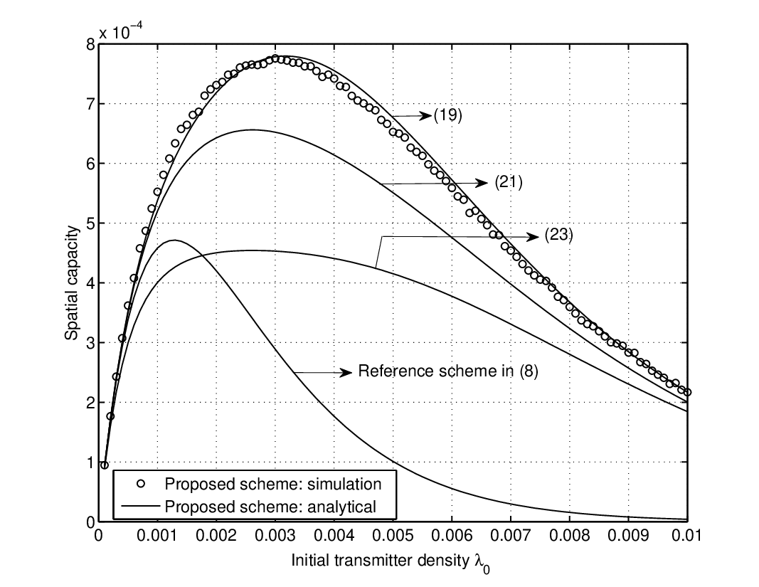
Fig. 3 shows the spatial capacity versus the initial transmitter density $\lambda_{0}$ when $\gamma_{1}<\beta$. We set $\gamma_{1}\!=\!0.6$. For the proposed scheme, similar to the case in Fig. 2, we observe tight and close approximates are provided by (19) and (21), respectively, based on the proposed approximate approach, while improper approximate is provided by (23) based on the conventional approximate approach. Moreover, it is observed that the spatial capacity of the proposed scheme is always larger than that of the reference scheme, given in (8), for all values of $\lambda_{0}$, which is as expected from Proposition III.1 since $\gamma_{1}\!<\!\beta$ in this example. Furthermore, for both the proposed and reference schemes, we observe an interesting density-capacity tradeoff: by increasing $\lambda_{0}$, the spatial capacity first increases due to more available transmitters, but as $\lambda_{0}$ exceeds a certain threshold, it starts to decrease, due to the more dominant interference effect. Thus, to maximize the spatial capacity, under the system scenario set in Fig. 3, the optimal $\lambda_{0}$ should be set as $0.003/m^{2}$.

We consider two existing distributed scheduling schemes for performance comparison. The first scheme is the iterative probability-based scheduling as in [18]. Denote the transmission probability for transmitter $i$ in P-Phase $k$, $1\leq k\leq N-1$, and the D-Phase as $\phi_{i}^{(k)}$ or $\phi_{i}^{(N)}$, respectively. For any $k\in\{1,..,N\}$, [18] sets $\phi_{i}^{(k)}=\min\left(\frac{\textrm{SIR}_{i}^{(k-1)}}{\beta},1\right)$. Intuitively, [18] provides a simple and proper way to iteratively adjust the transmission probability $\phi_{i}^{(k)}$. The second scheme is the channel-threshold based scheduling with single-stage probing as in [3] and [4], where the received interference power is not involved in the transmission decision and each transmitter decides to transmit in the D-Phase if its direct channel strength in P-Phase $0$ is no smaller than a predefined threshold $\gamma_{1}^{\prime}$, i.e., $h_{ii}\!\geq\!\gamma_{1}^{\prime}$. For a fair comparison, we consider single-stage probing with $N=1$ for all the proposed SIR-threshold based scheme, the probability-based scheduling in [18], and the channel-threshold based scheduling in [3] and [4].

Fig. 4 shows the spatial capacities achieved by the proposed scheme, the probability-based scheduling, the channel-threshold based scheduling, and the reference scheme without scheduling. To clearly show the effects of involving interference in the transmission decision for the proposed scheme, we set $\gamma_{1}^{\prime}\!=\!\gamma_{1}=0.4$ for the channel-threshold based scheduling. We obtain the spatial capacity of the channel-threshold based scheduling by applying its exact expression given in [4]. Due to the lack of an exact spatial capacity expression for the probability-based scheduling, we obtain its spatial capacity by simulation. We list our observations from Fig. 4 as follows:

• •

  SIR based schemes v.s. channel-threshold based scheme: It is observed that by adapting the transmission decision to the SIR, the achieved spatial capacities by both the proposed scheme and the probability-based scheduling are always higher than that by the channel-threshold based scheduling, where the interference information is not exploited. Moreover, the spatial capacity of the channel-threshold based scheduling is smaller than that of the reference scheme when $\lambda_{0}$ is small, and becomes larger when $\lambda_{0}$ is sufficiently large. This is in sharp contrast to the cases of the proposed scheme and the probability-based scheduling, which always guarantee capacity improvement over the reference scheme without scheduling.

• •

  SIR-threshold based scheduling v.s. probability-based scheduling: It is interesting to observe that although both the proposed scheme and the probability-based scheduling adapt the transmission decision to the SIR, the achieved spatial capacity by the former scheme is always higher than that by the latter one in this simulation. This is because that the proposed scheme assures the improvement of the successful transmission probability of each retained transmitter in the D-Phase, while the probability-based scheduling only assures such improvement with some probability. Moreover, it is observed that the optimal initial transmitter density that maximizes the spatial capacity of the proposed scheme is $\lambda_{0}^{*}=0.0036$, which is larger than that for the probability-based scheduling locating at $\lambda_{0}^{*}=0.0026$.

Note that for the proposed scheme, a lower SIR threshold $\gamma_{1}$ allows more transmitters to retain in the D-Phase, so as to have a second chance to transmit. Thus, by comparing the simulation results of the proposed scheme in Fig. 4 with that in Fig. 3, it is observed that the achieved optimal spatial capacity over $\lambda_{0}$ with $\gamma_{1}=0.4$ in Fig. 4 is larger than that with $\gamma_{1}=0.6$ in Fig. 3. In addition, for all the considered schemes in Fig. 4, we observe a density-capacity tradeoff, which is similar to that in Fig. 3.

We consider a more practical scenario, where SIR estimation and feedback errors exist in the implementation of the proposed scheme, and show the effects of the SIR errors on the spatial capacity. Similarly to [29], where the channel estimation and feedback errors are assumed to be zero-mean Gaussian variables, respectively, we assume the SIR estimation and feedback errors follow zero-mean Gaussian distributions with variance $\sigma^{2}_{est}$ and $\sigma^{2}_{fed}$, respectively. By further assuming that the two types of SIR errors are mutually independent, the sum of both SIR errors at transmitter $i$, denoted by $n_{i}$, follows zero-mean Gaussian distribution with variance $\sigma^{2}=\sigma^{2}_{est}+\sigma^{2}_{fed}$. Thus, in the presence of SIR errors, the feedback SIR level at transmitter $i$ in P-Phase 0 is $\textrm{SIR}_{i}^{(0)}+n_{i}$. Moreover, if the feedback SIR level $\textrm{SIR}_{i}^{(0)}+n_{i}\geq\gamma_{1}$ for a given SIR threshold $\gamma_{1}$ in P-Phase 1, transmitter $i$ decides to transmit in P-Phase $1$; otherwise, it decides to be idle in the remaining time of this time slot. Similar to its counterpart without SIR errors in Fig. 3 and Fig. 4, the spatial capacity with SIR errors is calculated as an average value over all the transmitters’ random locations, the random fading channels, as well as the random SIR errors.

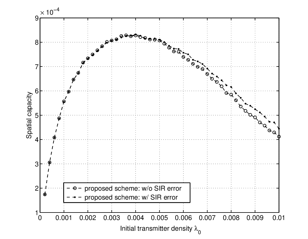
Fig. 5 numerically shows the spatial capacities of the proposed scheme in both cases with and without SIR errors. We set $\sigma^{2}=10^{-2}$ and $\gamma_{1}=0.4$ in this example. It is observed from Fig. 5 that when $\lambda_{0}$ is small, due to the resultant small interference in the network, each receiver $i$ feeds back a sufficiently high SIR level $\textrm{SIR}_{i}^{(0)}$ to its associated transmitter, such that $n_{i}$ has a small probability to affect the transmitter’s decision. Thus, we observe that when $\lambda_{0}$ is small, the spatial capacity with SIR errors is tight to that without SIR errors. However, as $\lambda_{0}$ increases, due to the decreased $\textrm{SIR}_{i}^{(0)}$ at each transmitter $i$, the transmitters become more easily affected by the SIR errors $n_{i}$ when deciding whether to transmit based on $\textrm{SIR}_{i}^{(0)}+n_{i}\geq\gamma_{1}$. It is noted that when $\lambda_{0}$ is sufficiently large, the average SIR level at each transmitter becomes very small; and even if $\textrm{SIR}_{i}^{(0)}\geq\gamma_{1}$ for transmitter $i$, $\textrm{SIR}_{i}^{(0)}$ is close to $\gamma_{1}$ with a large probability. Thus, under the case with zero-mean Gaussian distributed error $n_{i}$, for the transmitters with $\textrm{SIR}_{i}^{(0)}\geq\gamma_{1}$ in the SIR error-free case, it is more likely that these transmitters become $\textrm{SIR}_{i}^{(0)}+n_{i}<\gamma_{1}$ than $\textrm{SIR}_{i}^{(0)}+n_{i}\geq\gamma_{1}$ in the SIR error-involved case. Similarly, we can easily find that for the transmitters with $\textrm{SIR}_{i}^{(0)}<\gamma_{1}$ in the SIR error-free case, it is also more likely that these transmitters maintain $\textrm{SIR}_{i}^{(0)}+n_{i}<\gamma_{1}$ than $\textrm{SIR}_{i}^{(0)}+n_{i}\geq\gamma_{1}$ in the SIR error-involved case. Thus, the number of transmitters with $\textrm{SIR}_{i}^{(0)}+n_{i}<\gamma_{1}$ in the SIR error-involved case is larger than that with $\textrm{SIR}_{i}^{(0)}<\gamma_{1}$ in the SIR error-free case in general. Hence, as compared to the case without SIR errors, more transmitters will be refrained from transmitting in the D-Phase in the case with SIR errors, which improves the successful transmission probability in the D-Phase due to the reduced interference. As a result, it is interesting to observe from Fig. 5 that when the initial transmitter density $\lambda_{0}$ increases to some significant point, the spatial capacity with SIR errors becomes slightly higher than that without SIR errors; and their gap slowly increases over $\lambda_{0}$ after this point. Therefore, inaccurate SIR may even help improve the SIR-based scheduling performance in more interference-limited regime, which makes the proposed design robust to SIR errors.

References

- [1] S. Weber, J. G. Andrews, and N. Jindal, “An overview of the transmission capacity of wireless networks,” IEEE Trans. Commun., vol. 58, no. 12, pp. 3593-3604, Dec. 2010.
- [2] N. Jindal, S. Weber, and J. G. Andrews, “Fractional power control for decentralized wireless networks,” IEEE Trans. Wireless Commun., vol. 7, no. 12, pp. 5482-5492, Dec. 2008.
- [3] S. Weber, J. G. Andrews, and N. Jindal, “The effect of fading, channel inversion and threshold scheduling on ad hoc networks,” IEEE Trans. Inf. Theory, vol. 53, no. 11, pp. 4127-4149, Nov. 2007.
- [4] F. Baccelli, B. Blaszczyszyn, and P. Muhlethaler, “Stochastic analysis of spatial and opportunistic Aloha,” IEEE J. Sel. Areas Commun., pp. 1105-1119, Sep. 2009.
- [5] G. J. Foschini and Z. Miljanic, “A simple distributed autonomous power control algorithm and its convergence,” IEEE Trans. Veh. Technol., vol. 42, pp. 641–646, Nov. 1993.
- [6] R. D. Yates, “A framework for uplink power control in cellular radio systems,” IEEE J. Select Areas Commun., vol. 13, no. 7, pp. 1341-1347, Sep. 1995.
- [7] T. ElBatt and A. Ephremides, “Joint scheduling and power control for wireless ad hoc networks,” IEEE Trans. Wireless Commun., vol. 3, no. 1, pp. 74-85, Jan. 2004.
- [8] W. L. Huang and K. Letaief, “Cross-layer scheduling and power control combined with adaptive modulation for wireless ad hoc networks,” IEEE Trans. Commun., vol. 5, no. 4, pp. 728-739, Apr. 2007.
- [9] F. Baccelli and C. Singh, “Adaptive spatial aloha, fairness and stochastic geometry.” ” in Proc. IEEE Int. Symp. Modeling & Optimization in Mobile, Ad Hoc & Wireless Networks (WiOpt), May 2013.
- [10] P. Gupta and P. R. Kumar, “The capacity of wireless networks,” IEEE Trans. Inform. Theory, vol. 46, pp. 388-404, Mar. 2000.
- [11] M. Andrews and M. Dinitz, “Maximizing capacity in arbitrary wireless networks in the sinr model: complexity and game theory,” in Proc. IEEE Int. Conf. Computer Commun. (INFOCOM), Apr. 2009.
- [12] M. Dinitz, “Distributed algorithms for approximating wireless network capacity,” in Proc. IEEE Int. Conf. Computer Commun. (INFOCOM), Mar. 2010.
- [13] E. I. Asgeirsson and P. Mitra, “On a game theoretic approach to capacity maximization in wireless networks,” in Proc. IEEE Int. Conf. Computer Commun. (INFOCOM), Apr. 2011.
- [14] J. G. Andrews, R. K. Ganti, N. Jindal, M. Haenggi, and S. Weber, “A primer on spatial modeling and analysis in wireless networks,” IEEE Commun. Mag., vol. 48, no. 11, pp. 156-163, Nov. 2010.
- [15] D. Stoyan, W. S. Kendall, and J. Mecke, Stochastic geometry and its applications, 2nd edition. John Wiley and Sons, 1995.
- [16] A. Ghosh et al., “Heterogeneous cellular networks: From theory to practice,” IEEE Commun. Mag., vol. 50, no. 6, pp. 54-64, Jun. 2012.
- [17] J. Kingman, Poisson Processes. Oxford University Press, USA, 1993.
- [18] D. M. Kim and S. Kim, “Exploiting regional differences: A spatially adaptive random access.” Available [online] at http://arxiv.org/abs/1403.3891.
- [19] P. S. C. Thejaswi, J. Zhang, M.-O. Pun, H. V. Poor, and D. Zheng, “Distributed opportunistic scheduling with two-level probing,” IEEE/ACM Trans. Net., vol. 15, no. 5, pp. 1464-1477, Oct. 2010.
- [20] F. Baccelli, B. Blaszczyszyn, and P. Mühlethaler, “An ALOHA protocol for multihop mobile wireless networks,” IEEE Trans. Inform. Theory, vol. 52, no. 2, pp. 421-436, Feb. 2006.
- [21] D. Tse and S. Hanly, “Multiaccess fading channels–Part I: Polymatroid structure, optimal resource allocation and throughput capacities,” IEEE Trans. Inform. Theory, vol. 44, no. 7, pp. 2796-2815, Nov. 1998.
- [22] S. Hanly and D. Tse, “Multiaccess fading channels–Part II: Delay-limited capacities,” IEEE Trans. Inform. Theory, vol. 44, no. 7, pp. 2816-2831, Nov. 1998.
- [23] A. Hasan and J. G. Andrews, “The guard zone in wireless ad hoc networks,” IEEE Trans. Wireless Commun., vol. 6, pp. 897-906, Mar. 2007.
- [24] T. D. Novlan, H. S. Dhillon, and J. G. Andrews, “Analytical modeling of uplink cellular networks,” IEEE Trans. Wireless Commun., vol. 12, no. 6, pp. 2669-2679, Jun. 2013.
- [25] H. Q. Nguyen, F. Baccell, and D. Kofman, “A stochastic geometry analysis of dense IEEE 802.11 networks,” in Proc. IEEE Int. Conf. Computer Commun. (INFOCOM), 2007.
- [26] T. V. Nguyen and F. Baccelli, “A stochastic geometry model for cognitive radio networks,” The Computer Journal, vol. 55, pp. 534-552, Jul. 2011.
- [27] X. Song, C. Yin, D. Liu, and R. Zhang, “Spatial throughput characterization in cognitive radio networks with threshold-based opportunistic spectrum access,” IEEE J. Sel. Areas in Comm., to appear.
- [28] E. Hossain, L. Le, N. Devroye, and M. Vu, “Cognitive radio: from theory to practical network engineering,” in New directions in wireless communications research. Springer, 2009, ch. 10, pp. 251-289.
- [29] H. Su and E. Geraniotis, “Adaptive closed-loop power control with quantized feedback and loop filtering,” IEEE Trans. Wireless Commun., vol. 1, no. 1, pp. 76-86, Jan. 2002.
- [30] J. G. Andrews, F. Baccelli, and R. K. Ganti, “A tractable approach to coverage and rate in cellular networks,” IEEE Trans. Commun., vol. 59, no. 11, pp. 3122-3134, Nov. 2011.
- [31] M. Haenggi and R. K. Ganti, Inteference in large wireless networks. NOW: Foundations and Trends in Networking, 2008.
- [32] C. P. Niculescu and J. Pečarić, “The equivalence of Chebyshev’s inequality with the Hermite-Hadamard inequality,” Math. Reports, vol. 12(62), no. 2, pp. 145-156, 2010.
- [33] J. Chamberland and V. V. Veeravalli, “Decentralized dynamic power control for cellular CDMA Systems,” IEEE Trans. Wireless Commun., vol. 2, no. 3, pp. 549-559, May. 2003.