Phase diagram of non-degenerate twisted mass fermions

It has long been known, in the case of three light quarks, that there is a transition to a CP-violating phase for non-degenerate quarks when one of the quark masses becomes sufficiently negative [1]. For example, using leading order (LO) SU(3) chiral perturbation theory ($\chi$PT), and fixing $m_{d}$ and $m_{s}$, the transition occurs when $m_{u}=-m_{d}m_{s}/(m_{d}+m_{s})$ [2]. The neutral pion becomes massless on the transition line, and within the new phase the chiral order parameter, $\langle\Sigma\rangle$, becomes complex. For physical QCD this is mostly a curiosity, since increasingly accurate determinations of the quark masses indicate clearly that all are positive relative to one another [3, 4]. Thus physical QCD, despite the non-degeneracy of the up and down quarks, lies away from the critical line.

For lattice QCD (LQCD), however, the situation is less clear. The position of the transition can be shifted closer to the physical point by discretization effects. Indeed, it is well known that, with degenerate Wilson-like fermions,¹¹ 1 “Wilson-like” indicates that the analysis holds for both Wilson fermions and various improvements thereof, in particular for non-perturbatively ${\cal O}(a)$-improved Wilson fermions. discretization effects can lead to the appearance of a new phase—the Aoki phase—in which isospin is spontaneously broken and $\langle\Sigma\rangle$ is complex [5, 6]. In addition, advances in simulations now allow calculations to be done at the physical light-quark masses, including, very recently, the physical non-degeneracy between up and down quarks [7]. It is thus natural to ask how, in LQCD with non-degenerate quarks, discretization effects change the position and nature of the CP-violating phase. This question is particularly acute in the case of twisted-mass fermions, where additional symmetry breaking is explicitly included.

In this paper we address this question for Wilson-like and twisted-mass lattice fermions. We do so using $\chi$PT, specifically the versions of $\chi$PT in which the effects of discretization have been included. Our work also allows us to address a related issue: In what way is the CP-violating phase of the continuum theory related to the Aoki phase of the lattice theory?²² 2 This issue has been raised previously by Mike Creutz and his conjectured answer is confirmed by the present analysis [8].

Since twisted-mass QCD is only defined for even numbers of fermion flavors [9], a necessary step for our work is to rephrase the continuum SU(3) $\chi$PT analysis of Ref. [2] in the two-flavor theory obtained by integrating out the strange quark. This requires that the contributions of one of the next-to-leading order (NLO) low-energy coefficients ($\ell_{7}$) be treated as parametrically larger than the others. Thus we are led to a somewhat non-standard power-counting, but one which reproduces the SU(3) phase diagram, including the CP-violating phase, within SU(2) $\chi$PT. This approach has been used before along the line $m_{u}=-m_{d}$ [10]; here we extend the analysis to arbitrary mass splitting. Similar work has also been done recently in the context of a effective theory including the $\eta$ meson [11].

The organization of this article is as follows. In Sec. II we briefly recall the results for the phase structure and pion masses at LO in SU(2) and SU(3) $\chi$PT, and show how they differ. Section III describes the matching of SU(3) and SU(2) $\chi$PT. In Sec. IV, we recall briefly how discretization effects are incorporated in $\chi$PT for degenerate Wilson-like fermions, and the resulting phase structure. We then present our first new results: the phase diagram including both discretization effects and non-degeneracy. In Sec. V we move onto twisted-mass fermions, focusing first on the phase diagram and pion masses in the case of maximal twist, where most simulations have been done because of the property of automatic $\mathcal{O}(a)$ improvement [9]. It is nevertheless interesting to understand how the results with untwisted and maximally twisted fermions are connected, and so, in Sec. VI, we discuss the phase diagram for general twist.

Up to this stage, our analysis is done using the LO terms due to the average quark mass, discretization effects and non-degenerate quark masses. To understand how robust the results are we consider, in Sec. VII, the impact of including the next higher order terms in our power counting. Some conclusions are collected in Section VIII.

In this section we review the vacuum structure predicted by LO $\chi$PT for both two and three light flavors. The LO chiral Lagrangian in Euclidean space-time is, for any number of light flavors,

where $\Sigma\in SU(N_{f})$ and $\chi=2B_{0}M$ (with $M$ the mass matrix), while $f\sim 92\;$MeV and $B_{0}$ are low-energy constants (LECs).

For two light flavors the chiral order parameter can be parametrized as $\langle\Sigma\rangle=\exp(i\theta\hat{n}\cdot\vec{\tau})$. Although the mass matrix $M={\rm diag}(m_{u},m_{d})$ has both singlet and triplet components, the leading order potential depends only on the former

In the last step we have defined the convenient quantity $\chi_{\ell}=B_{0}(m_{u}+m_{d})$. The potential is minimized at $\theta=0$ if $\chi_{\ell}>0$ and at $\theta=\pi$ if $\chi_{\ell}<0$, resulting in the phase diagram sketched in Fig. 1. In terms of the behavior of the condensate, this is a first-order phase transition at which the condensate flips sign. This characterization is somewhat misleading, however, because the two sides of the transition are related by a non-anomalous flavor rotation. Such a transformation can change $M\to-M$ and $\Sigma\to-\Sigma$, while leaving physics unchanged. Thus by adding an extra dimension to the phase diagram (as we will do later) one finds that the two sides are connected.

Expanding the potential about its minimum, using $\Sigma=\langle\Sigma\rangle\exp(i\vec{\pi}\cdot\vec{\tau}/f)$ we find the standard LO result for the pion masses, $m^{2}_{\pi}=|\chi_{\ell}|$. These thus vanish along the phase transition line. That they vanish at the origin follows from Goldstone’s theorem due to the spontaneous breaking of the exact axial symmetry. That they vanish away from the origin along the transition line is not expected from symmetry arguments, and indeed holds, as we will see, only at LO in $\chi$PT.

The phase diagram of the three-flavor theory has a more interesting structure, as elucidated most extensively by Creutz [2]. Since $m_{s}\gg m_{u},m_{d}$ in nature, it is natural to hold $m_{s}$ fixed and vary the other two quark masses. The resulting phase diagram at LO is sketched in Fig. 2. The “normal” region, in which $\langle\Sigma\rangle=\mathbb{1}$, ends at a transition line along which $m_{\pi^{0}}$ vanishes. This occurs (for fixed $m_{s}>0$) when one of the other masses, say $m_{u}$, becomes sufficiently negative. The explicit expression for the neutral pion mass in this phase is

which vanishes when $m_{u}=-m_{d}m_{s}/(m_{d}+m_{s})$. The charged pions remain massive throughout the normal phase except at the origin.

Moving outside the normal phase one enters a CP-violating phase in which the condensate is complex. The explicit form is

where the phases satisfy

In this case there is a genuine phase transition at the boundary. It is of second order: $\langle\Sigma\rangle$ is continuous, and a single pion becomes massless.

The phase diagram is symmetric under both $m_{u}\leftrightarrow m_{d}$ interchange and inversion through the origin (with $m_{s}$ fixed). Inversion is brought about by a non-anomalous axial isospin transformation, which also changes the condensate as shown in Fig. 2. We note that the CP-violating region is of finite width.³³ 3 The theory along the $m_{u}=-m_{d}$ diagonal is identical to that with $m_{u}=m_{d}$ at $\theta_{\rm QCD}=\pi$, and has been discussed extensively in the literature. In particular, a $\chi$PT analysis of this theory has been given in Ref. [10]. Specifically, as one moves away from the origin along the $m_{u}=-m_{d}$ diagonal, the width of this region grows proportionally to $(m_{u}\!-\!m_{d})^{2}/m_{s}$.

As the figure shows, there are additional phase boundaries in the second and fourth quadrants. These occur, however, when $|m_{u}|,|m_{d}|>|m_{s}|$, and thus lie far from the region of physical interest. In the rest of our analysis, we consider only the region in which $|m_{u}|,|m_{d}|\ll|m_{s}|$, and thus zoom in on the vicinity of the origin in Fig. 2.

If we choose the quark masses to satisfy $|m_{u}|,|m_{d}|\ll|m_{s}|\ll\Lambda_{\rm QCD}$, then the properties of pions can be simultaneously described by both SU(2) and SU(3) $\chi$PT, and the predictions of the two theories must agree. The results of the previous section show that this is not the case if we work to LO in both theories—the CP-violating phase is absent in SU(2) $\chi$PT. The discrepancy is resolved by noting that the CP-violating phase has a width proportional to $(m_{u}\!-\!m_{d})^{2}$, indicating that it arises at NLO in SU(2) $\chi$PT. In this section we recall how the two theories are matched, and show how the CP-violating phase can then be obtained in SU(2) $\chi$PT when including the resulting NLO term.

To do the matching, one considers quantities accessible in both SU(2) and SU(3) theories, namely pion masses and scattering amplitudes. Expanding the LO SU(3) result in powers of $m_{u,d}/m_{s}$, the leading terms match with the LO SU(2) result, while the first subleading terms match with an NLO SU(2) contribution. The subleading terms in the SU(3) results are in fact proportional to $(m_{u}\!-\!m_{d})^{2}$, because they arise from intermediate $\eta$ propagators and involve two factors of the $\pi^{0}-\eta$ mixing amplitude. The only source of such mass dependence at NLO in the SU(2) theory is the $\ell_{7}$ term in the NLO potential

Writing $\chi$ as

we see that only the $\epsilon$ part contributes to the $\ell_{7}$ term. Thus this term leads to contributions proportional to $(m_{u}\!-\!m_{d})^{2}$. Other NLO contributions (i.e. those proportional to different NLO LECs or coming from loops) do not have this mass dependence.

The simplest quantity with which to do the matching is the neutral pion mass, and this was used to determine the value of $\ell_{7}$ in Ref. [12]. The LO SU(3) result [given in Eq. (3) above] expands to

The SU(2) result at NLO is

where $\Lambda_{\chi}=4\pi f$ is the chiral scale. The $\chi_{\ell}^{2}$ contributions arise from terms in the NLO chiral Lagrangian (including $\ell_{3}$) as well as from chiral logarithms. Equating these two results one finds [12]

One can show that with this value for $\ell_{7}$, contributions to all pion $n$-point amplitudes proportional to $\epsilon^{2}/m_{s}$ agree in the two theories.

We stress that in this matching we are not taking into account “standard” NLO contributions, i.e. those suppressed relative to LO results by factors of $m_{u,d}/\Lambda_{\rm QCD}\sim(m_{\pi}/\Lambda_{\chi})^{2}$ (up to logarithms). Such contributions arise in both SU(3) and SU(2) $\chi$PT and must be included in a full NLO matching. This is not necessary for our purposes since such terms lead to small isospin-conserving corrections to the vacuum structure and pion masses—they do not introduce qualitatively new effects. By contrast, the $\epsilon^{2}$ terms that we keep lead to isospin breaking, and are the leading order contributions which do so. Indeed, for this reason $\ell_{7}$ is not renormalized at this order, since, as already noted, one-loop chiral logarithms do not contain a term proportional to $\epsilon^{2}$. Thus it is consistent to work with the classical potential, rather than the one-loop effective potential. This is not the case for other LECs such as $\ell_{3}$, which are renormalized and thus scale-dependent [12].

We can formalize this by noting that standard NLO contributions are parametrically smaller than the terms we keep by a factor of $m_{s}/\Lambda_{\rm QCD}$. This allows the development of a consistent power-counting scheme in which the $\epsilon^{2}$ terms are larger than generic $m^{2}$ contributions.⁴⁴ 4 The numerical basis for this power-counting is not very strong. For example, $\ell_{7}$ and $\ell_{3}(\mu)$ are comparable in size for reasonable values of the scale $\mu$. Thus the numerical size of the standard NLO corrections we are dropping may be comparable to those proportional to $\epsilon^{2}$ that we are keeping. The key point, however, is that we are interested in qualitatively new effects, rather than a precise quantitative description. We discuss this in the following section. To be consistent we should also account for NLO contributions in SU(3) $\chi$PT of size $m_{s}/\Lambda_{\rm QCD}$ relative to LO terms. These, however, lead only to a renormalization of the SU(2) constants $f$ and $B_{0}$ relative to their SU(3) counterparts. Since we work henceforth entirely in the SU(2) theory, we choose to leave this renormalization implicit.

We now show that the inclusion of the $\ell_{7}$ term leads to the same phase diagram as found in the LO SU(3) analysis. Given the matching result Eq. (10), we always assume $\ell_{7}>0$ in the following. Using $\langle\Sigma\rangle=\exp(i\theta\hat{n}\cdot\vec{\tau})$, the potential becomes

where $c_{\ell}=\ell_{7}/f^{2}$. Since $\ell_{7}>0$, the potential is always minimized by choosing $|n_{3}|=1$. Since $n_{3}=1$ and $n_{3}=-1$ are related by changing the sign of $\theta$, we can, without loss of generality, set $n_{3}=1$. The resulting potential is stationary with respect to $\theta$ at the “normal” values $\theta=0$ and $\pi$, and in addition at

This new stationary value always leads to the global minimum of the potential where it is valid, i.e. when $|\cos\theta|\leq 1$. Thus, for fixed $\epsilon$, there is a new phase for $-2c_{\ell}\epsilon^{2}\leq\chi_{\ell}\leq 2c_{\ell}\epsilon^{2}$, within which $\langle\Sigma\rangle$ is complex and CP is violated. Although $\cos\theta$ is fixed, the sign of $\theta$ is not, with the two possible vacua begin related by a CP transformation. This phase matches continuously onto the normal phases with $\cos\theta=\pm 1$ at its boundaries. Thus the phase transition is of second order.

The resulting phase diagram is sketched in Fig. 3. This is not only qualitatively similar to the central portion of the LO SU(3) phase diagram, Fig. 2, but is in fact in complete quantitative agreement at the appropriate order. For example, expanding the SU(3) result for the phase boundary, $m_{u}=-m_{d}/(1+m_{d}/m_{s})$, in powers of $m_{u,d}/m_{s}$, and keeping only the leading non-trivial term, one finds that the boundary occurs at $\chi_{\ell}=\epsilon^{2}/(4B_{0}m_{s})$. This agrees with the SU(2) result $\chi_{\ell}=2\ell_{7}\epsilon^{2}/f^{2}$ using the matching condition (10). We have also checked that the pion masses agree throughout the phase plane. We do not quote results for pion masses here, since they are included in the more general analysis presented below.

The fact that the CP-violating phase can be reproduced within SU(2) $\chi$PT was first explained by Smilga [10]. His work considered only the case $m_{u}=-m_{d}$, which, as noted above, is the same as $m_{u}=m_{d}$ with $\theta_{\rm QCD}=\pi$. The analysis presented here gives the (very simple) generalization to arbitrary non-degenerate quark masses. There is also a close relation between our analysis and the recent work of Aoki and Creutz [11]. These authors do not use $\chi$PT per se, but rather an effective theory containing both pions and the $\eta$ meson. If the $\eta$ were integrated out then their theory would reduce to that we consider here, including the $\ell_{7}$ term, plus small corrections. We think, however, that it is preferable to work in a strict effective theory framework, in which only the light particles are kept as dynamical degrees of freedom.

In this section we recall how lattice artifacts can be incorporated into $\chi$PT, and study their impact on the phase structure described above at leading non-trivial order. We do this for untwisted Wilson-like fermions—twist will be considered in the following sections. The method leads to the chiral effective theory describing lattice simulations close to the continuum limit. We begin by recalling the analysis for degenerate quarks and then add in non-degeneracy. We work entirely in the two-flavor theory obtained after the strange quark (and the charm quark too, if present) has been integrated out. For untwisted Wilson-like fermions (unlike for twisted-mass fermions), the analysis could also be carried out within SU(3) $\chi$PT, but there is no advantage to doing so as the dominant long-distance dynamics lies in the SU(2) sector.

Both quark masses and discretization effects break chiral symmetry, and it is important to understand the relative size of these effects. Our focus here is on state-of-the-art simulations, which have $m_{u,d}$ close to their physical values ($m_{u}\approx 2.5\;$MeV and $m_{d}\approx 5\;$MeV in the $\overline{\rm MS}$ scheme at $\mu=2\;$GeV), and lattice spacings such that $1/a\approx 3\;$GeV. In this case, the relative size of discretization effects is characterized by $a\Lambda_{\rm QCD}\approx 0.1$ (using $\Lambda_{\rm QCD}=300\;$MeV), so that

The appropriate power-counting is thus (in schematic notation) $a^{2}\sim m$. This is the Aoki regime, in which competition between discretization and mass effects leads to interesting phase structure [5, 6].

Discretization effects can be incorporated into $\chi$PT following the method of Ref. [6]. For unimproved (or partially improved) Wilson fermions, the dominant discretization effect is proportional to $a$. In the pion sector, however, this contribution can be absorbed entirely into a common shift in all quark masses [6], and we assume below that this shift has been made. The first non-trivial discretization effect is that proportional to $a^{2}$. This changes the LO potential to [6]

Here we are using the notation of Ref. [13], in which $\hat{A}=2W_{0}a\mathbb{1}$ is a spurion field, with dimensions of mass squared, and proportional to the identity matrix in flavor space. $W_{0}$ and $W^{\prime}$ are new LECs.

The analysis of the vacuum structure for degenerate quarks was given in Ref. [6]. Since ${\cal V}_{a^{2}}$ is independent of the $\epsilon$, the results are unchanged at LO in the presence of non-degeneracy. To determine the vacuum we must minimize

where $w^{\prime}={64W^{\prime}W_{0}^{2}a^{2}}/{f^{2}}$. For $w^{\prime}<0$, the analysis is essentially the same as that for ${\cal V}_{SU(2)}$ with $\ell_{7}>0$, as given in the previous section. Stationary points are at $\cos\theta=\pm 1$ and

with the latter being the global minimum where valid ($|\cos\theta|\leq 1$). This leads to the phase diagram shown in Fig. 4, with an Aoki phase [5] separated from the normal phases by second-order transitions at $|\chi_{\ell}|=-2w^{\prime}$. Strictly speaking, the name “Aoki phase” has been applied previously only on the diagonal $m_{u}=m_{d}$ axis, but in the present approximation it holds also for non-degenerate quarks. Within the Aoki phase the potential is independent of the direction of the condensate, $\hat{n}$, so that there are two massless Goldstone bosons, the charged pions. Parity and flavor are violated within this phase. With the canonical choice of the direction of the condensate, $\hat{n}=\hat{z}$, CP is also violated.

For $w^{\prime}>0$, the global minimum lies at $\cos\theta={\rm sign}(\chi_{\ell})$, with a first-order transition at $\chi_{\ell}=0$. The phase diagram is thus identical to that in the continuum, Fig. 1. The only difference is that here the yellow line indicates a genuine first-order transition, since on the lattice there are no symmetries connecting the two sides. This case is referred to as the first-order scenario [6].

We are now ready to combine the effects of non-degeneracy with discretization errors. This requires that we adopt an appropriate power-counting scheme for the relative importance of $\epsilon^{2}$, $m$ and $a^{2}$, where $m$ indicates a generic quark mass. Recalling that $\epsilon^{2}$ terms are enhanced compared to generic $m^{2}$ terms we use

This can be thought of as treating $\epsilon\sim a^{1+\delta}$, with $0<\delta<1/2$. The utility of this power counting is that allows us to first add the $\epsilon^{2}$ term to those proportional to $m$ and $a^{2}$, and then consider terms of order $ma\sim a^{3}$ at a later stage (in Sec. VII below). Indeed, we could, for the purposes of this section, set $\delta=0$, and treat the $\epsilon^{2}$ term as of LO. We do not do so, however, since this would require us to later treat $a\epsilon^{2}$ terms as of the same size as those proportional to $ma\sim a^{3}$. Nevertheless, we will loosely describe the inclusion of $m$, $a^{2}$ and $\epsilon^{2}$ terms as constituting our LO analysis, while treating the $ma\sim a^{3}$ terms as being of NLO. Terms of yet higher order will not be considered.

With the power counting in hand, we can extend the inclusion of discretization errors into $\chi$PT to incorporate the effects of non-degeneracy. This leads to the appearance of new operators in the Symanzik effective Lagrangian, and thus, potentially, to new terms in the chiral Lagrangian. The constraints on additional operators in the Symanzik Lagrangian in the presence of non-degeneracy were worked out in Ref. [14]. Using their results within our power-counting scheme, we find that the lowest order new operator is $\sim a\epsilon^{2}\bar{\psi}\psi$. This is, however, of higher order than we consider here.⁵⁵ 5 Furthermore, when mapped to the chiral Lagrangian, it leads to contributions which can be absorbed by making the untwisted mass $m$ have a weak dependence on $\epsilon$. Thus it does not lead to new phases, but only to a small distortion of the phase diagram. All other operators are of yet higher order. Thus, at the order we work, non-degeneracy only enters our calculation through the continuum $\ell_{7}$ term. The LO potential thus becomes

We stress that it is self-consistent to determine the vacuum structure and pion masses from a tree-level analysis of ${\cal V}_{a^{2},\ell_{7}}$ since loop effects only come in at ${\cal O}(m^{2},ma^{2},a^{4})$.

In terms of the parameters of $\langle\Sigma\rangle$, the potential is now given by

As before, we can set $n_{3}=1$ without loss of generality. The stationary points are at $\cos{\theta}=\pm 1$ and

The latter minimizes the potential if $c_{\ell}\epsilon^{2}-w^{\prime}>0$ and is valid for $|\cos\theta|\leq 1$. This results in the phase diagrams of Figs. 5(a) and 5(b) for $w^{\prime}<0$ and $w^{\prime}>0$, respectively. In the former case, corresponding to the Aoki phase for degenerate quarks, the second-order transition lines lie at

Thus the width of the phase grows as $|\epsilon|$ increases. Furthermore, comparing to Fig. 4, we see that the continuum CP-violating phase and the Aoki phase are continuously connected.⁶⁶ 6 This result is in agreement with Creutz’ conjecture [8]. The only subtlety in this connection is that the condensate definitely points in the $n_{3}$ direction for $\epsilon\neq 0$ (i.e. the direction picked out by the non-degenerate part of the mass term), whereas for $\epsilon=0$ the direction is arbitrary.

In the first-order scenario, Fig. 5(b), the first-order transition along the $m_{u}=-m_{d}$ line weakens as $|\epsilon|$ increases, until, at $c_{\ell}\epsilon^{2}=w^{\prime}$, the CP-violating phase appears. The second-order transition lines are then given by $|\chi_{\ell}|=2(c_{\ell}\epsilon^{2}-w^{\prime})$, i.e. by the same equation as in the Aoki scenario.

We next calculate the pion masses throughout the phase plane, expanding about the vacuum as

Outside the CP-violating phase, we find

while within the CP-violating phase we have

where $\theta$ is given in Eq. (20). These results are plotted versus $\chi_{\ell}$ for various characteristic choices of $\epsilon$ and $w^{\prime}$ in Fig. 6.

Figures 6a and b show the continuum results for degenerate and non-degenerate masses, respectively. The neutral pion mass vanishes along the second-order transition line, as expected. The full degeneracy at $\chi_{\ell}=0$ is due to the fact that the theory regains flavor symmetry (with $\theta_{\rm QCD}=\pi$) at this point. A characteristic feature of the spectrum at this order is that the charged pion mass is independent of $\chi_{\ell}$ within the CP-violating phase. This holds also when discretization errors are included.

Figures 6c and d show the spectrum for degenerate quarks with discretization errors included, respectively for the Aoki and first-order scenarios, reproducing the results of Ref. [6].

Our new results are those of Figs. 6e-g, which include the effects of both discretization errors and non-degeneracy. In this case the charged and neutral pion masses differ in general. Figure 6e shows the behavior in the Aoki scenario, where $m_{\pi^{0}}$ vanishes on the phase transition lines, and rises above $m_{\pi^{\pm}}$ in the central region of the CP-violating phase. There are thus two values of $\chi_{\ell}$ where all pions are degenerate, but these are accidental degeneracies and not indicative of any symmetry. For the first-order scenario Fig. 6f shows the spectrum when $\epsilon$ is chosen so that the plot passes through the end-point of the second-order transition line, while Fig. 6g shows what happens as one moves through the CP-violating phase. In this case, there are no degenerate points.

Simulations using Wilson-like fermions at physical masses, including isospin breaking, have recently begun [7]. What is the significance of our results for such simulations? The main issue is whether discretization effects can move the CP-violating phase such that it lies closer to, or even includes, the physical point. Clearly one wants to avoid simulating in this phase, since it has a different vacuum structure from the continuum theory. But even lying close to a second-order transition could lead to algorithmic issues due to critical slowing down. What we have found is that the phase does move closer to the physical point in the Aoki scenario, Fig. 5(a). In this scenario, the CP-violating phase now includes a region of positive quark masses. On the other hand, for the first-order scenario, discretization effects move the CP-violating phase away from the physical point. A positive aspect of our results is that discretization errors lead only to a overall shift in pion masses (outside of the CP-violating phase), so that the difference $m_{\pi^{\pm}}^{2}-m_{\pi^{0}}^{2}$ takes its continuum value $2c_{\ell}\epsilon^{2}$ in both scenarios.

In this section we extend the previous analysis to twisted-mass fermions [15] at maximal twist. Such fermions have the important practical property of automatic ${\cal O}(a)$ improvement [9]. They are being used to simulate QCD with quarks at or near their physical masses [16, 17], and isospin breaking is now being included [18]. The main question we address here is the same as for untwisted fermions: How do discretization effects change the continuum phase structure and pion masses?

In the continuum, twisted mass fermions are obtained by a non-anomalous axial rotation,

with $m_{\ell}=(m_{u}\!+\!m_{d})/2$, $\epsilon_{\ell}=(m_{u}\!-\!m_{d})/2$, $m=m_{\ell}\cos\omega$, $\mu=m_{\ell}\sin\omega$, and $\omega$ the twist angle. Conventionally, $m$ is called the untwisted (average) mass and $\mu$ the twisted (average) mass. Choosing the twist in a direction orthogonal to $\tau_{3}$ leaves the $\epsilon_{\ell}$ term unchanged. In the continuum this is a convenience, but not a necessity. Once one discretizes $\not{D}$ with a Wilson term, however, it is mandatory to twist in a direction orthogonal to $\tau_{3}$ if one wants to keep the fermion determinant real [19].⁷⁷ 7 In Ref. [18], which studies twisted-mass non-degenerate fermions, the twist is chosen in the $\tau_{3}$ direction. This leads to a complex fermion determinant, which is avoided in practice by perturbing at linear order around the isospin-symmetric theory. Because the twist is in the $\tau_{3}$ direction, our present results do not apply to these simulations. We will discuss the generalization to $\tau_{3}$ twist (along with the inclusion of electromagnetism) in an upcoming work [20]. By convention, this direction is chosen to be $\tau_{1}$. The rescaled mass matrix that enters $\chi$PT is now

and is no longer hermitian. Here we have defined

following Ref. [13].

To determine the effective chiral theory for twisted-mass lattice QCD the first step is to determine the additional operators in the Symanzik Lagrangian that are induced by twisting. As in the untwisted case, the form of the allowed operators can be obtained from the analysis of Ref. [14], which includes both twist and non-degeneracy. In fact, since $\widehat{\mu}^{2}$ is smaller than $\epsilon^{2}$ in our power-counting, the inclusion of twist does not change the result for the untwisted case, namely that the lowest order new operator is $\sim a\epsilon^{2}$ and of higher order than we are working. Thus at LO the extension $\chi$PT to include twist and discretization errors is accomplished by simply using the twisted $\chi$ of Eq. (28) in the potential ${\cal V}_{a^{2},\ell_{7}}$ of Eq. (18).

Using our standard parametrization of $\langle\Sigma\rangle$ this gives

We focus in this section on the case of maximal twist, $\widehat{m}=0$, where simple analytic results can be obtained. Even with this simplification, we note that there is competition between terms in three directions in $\Sigma$: the twist direction $n_{1}$, the non-degeneracy direction $n_{3}$, and the identity direction ($w^{\prime}$ term). Thus we can expect a more complicated phase structure than for untwisted Wilson fermions. Furthermore, since non-degenerate twisted-mass quarks completely break the continuous SU(2) flavor symmetry, we expect, in general, that all three pion masses will differ.

We find the phase diagrams shown in Fig. 7. Note that we are now plotting the average mass along the vertical axis and the difference horizontally. We do this because $\widehat{\mu}$ and $\epsilon$ are proportional to parameters that enter the twisted-mass lattice action. To compare to the earlier plots, one should rotate those of Fig. 7 by $45^{\circ}$ in a clockwise direction. We see that, at maximal twist, it is the Aoki scenario which is preferred, in the sense that the CP-violating phase does not move closer to the physical point. Indeed, the phase diagram in this scenario is identical to that in the continuum, Fig. 3, with the replacement $\chi_{\ell}\to\widehat{\mu}$. In the first-order scenario, by contrast, there is an additional phase (colored green in Fig. 7b) which brings lattice artifacts closer to the physical point. Thus the relative merits of the two scenarios are interchanged compared to the untwisted case.

To understand the phase diagrams we first recall the result for the degenerate case, $\epsilon=0$, which has been studied in Refs. [21, 22, 13]. These works find, for large $|\widehat{\mu}|$, that the condensate is aligned with the twist, i.e. $n_{1}=1$ and $\sin\theta={\rm sign}(\widehat{\mu})$. This is as in the continuum. In the Aoki scenario ($w^{\prime}<0$), this alignment holds for all $\widehat{\mu}$, and there is a first-order transition at $\widehat{\mu}=0$ where $\sin\theta$ changes sign. In the first-order scenario ($w^{\prime}>0$), there are second-order transitions at the two points $\widehat{\mu}=\pm 2w^{\prime}$, at which one of the pion masses vanishes. For $|\widehat{\mu}|<2w^{\prime}$ the condensate smoothly rotates within the group manifold with $\sin\theta=\widehat{\mu}/(2w^{\prime})$. These features are reproduced by our results along the vertical axes in Fig. 7.

We now explain how these results are generalized to $\epsilon\neq 0$. We first observe that we can set $n_{2}=0$. This is because, for any choice of $n_{1}$, the $c_{\ell}$ term in Eq. (30) (with $c_{\ell}>0$) will be minimized when $n_{3}^{2}$ is maximized, i.e. with $n_{3}^{2}=1-n_{1}^{2}$. Thus there are only two independent variables, $\theta$ and $n_{1}$. Since $n_{1}$ satisfies $|n_{1}|\leq 1$, we parametrize it as $n_{1}=\cos\varphi_{1}$. Since $\langle\Sigma\rangle$ is invariant when $\theta$ and $\vec{n}$ change sign, we need only consider $n_{1}\geq 0$, i.e. $0\leq\varphi_{1}\leq\pi/2$. The stationary points are obtained from simultaneously solving

The solutions are

1. 1.

   $\cos\theta=0$ (so that $\sin\theta=\pm 1$) together with $\sin\varphi_{1}=0$ (so that $n_{1}=1$). In these cases ${\mathcal{V}_{a^{2},\ell_{7}}}/{f^{2}}=\mp\widehat{\mu}$, so that the solution with the lowest energy is that with $\sin\theta={\rm sign}(\widehat{\mu})$, giving ${\mathcal{V}_{a^{2},\ell_{7}}}/{f^{2}}=-|\widehat{\mu}|$.

2. 2.

   $\sin\theta={\rm sign}(\widehat{\mu})$ and $n_{1}=\cos\varphi_{1}={|\widehat{\mu}|}/({2c_{\ell}\epsilon^{2}})$ so that ${\mathcal{V}_{a^{2},\ell_{7}}}/{f^{2}}=-{\widehat{\mu}^{2}}/({4c_{\ell}\epsilon^{2}})-c_{\ell}\epsilon^{2}$. This is only valid when $n_{1}\leq 1$, i.e. $|\widehat{\mu}|\leq 2c_{\ell}\epsilon^{2}$. There are two degenerate solutions, with $n_{3}=\pm\sin\varphi_{1}$.

3. 3.

   $\sin\theta=\widehat{\mu}/(2w^{\prime})$ and $\varphi_{1}=0$ (implying $n_{1}=1$) so that ${\mathcal{V}_{a^{2},\ell_{7}}}/{f^{2}}=-\widehat{\mu}^{2}/(4w^{\prime})-w^{\prime}$. This is only valid when $|\widehat{\mu}|\leq 2w^{\prime}$. There are two degenerate solutions, with opposite signs of $\cos\theta$.

4. 4.

   $\cos\theta=\pm 1$ and $\widehat{\mu}n_{1}=0$, so that $\mathcal{V}_{a^{2},\ell_{7}}/f^{2}=-w^{\prime}$. This never has lower energy than the third solution and can be ignored.

The first solution is the continuum one discussed above. The second has lower energy than the first where it is valid, and goes over to the CP-violating phase when $w^{\prime}=0$. The third solution is relevant only for $w^{\prime}>0$, in which case it has the lowest energy when $c_{\ell}\epsilon^{2}<w^{\prime}$. The condensate in this phase is independent of $\epsilon$. These considerations lead to the phase diagrams shown in Fig. 7. The potential is continuous throughout the phase planes, as is the condensate except at the junction between the central (green colored) phase and the CP-violating phase in Fig. 7b. Thus we expect the transitions to be of second order.

We calculate pion masses using the parametrization

Here we are using an axial transformation to rotate from the twisted basis to the physical basis, which ensures, in the continuum, that the pion fields have physical flavors [23]. In the continuum-like phase (uncolored in the figures), which lies in the regions $|\widehat{\mu}|\geq{\rm max}(2c_{\ell}\epsilon^{2},2w^{\prime})$, we find

These results are consistent with those of Ref. [24], where a $\chi$PT calculation in this phase is carried out using the different power-counting $m\gtrsim a$. Various aspects of these results are noteworthy. First, all three masses differ. This is expected since flavor symmetry is completely broken. Second, the charged pions are not mass eigenstates; instead, the eigenstates are $\pi_{1,2}$ and the neutral pion. These two points were also noted in Ref. [24]. Third, one of the pion masses vanishes at each of the phase boundaries: $m_{\pi_{3}}$ at the boundary with the CP-violating (pink colored) phase, and $m_{\pi_{1}}$ at the boundary with the central (green colored) phase in the first-order scenario.⁸⁸ 8 In the degenerate case ($\epsilon=0$) Refs. [21, 22, 13] find that it is $m_{\pi_{3}}$ which vanishes at $|\widehat{\mu}|=2w^{\prime}$, rather than $m_{\pi_{1}}$. This difference arises because we twist in the $\tau_{1}$ direction rather than the $\tau_{3}$ direction used in Refs. [21, 22, 13]. This is expected since these are continuous transitions at which a $Z_{2}$ symmetry is broken ($\theta\to-\theta$ for the “green phase” and $n_{3}\to-n_{3}$ for the CP-violating phase). Finally, in the first-order scenario, there are four tricritical points at which both $m_{\pi_{3}}$ and $m_{\pi_{1}}$ vanish. These occur where all three phases meet, i.e. at $|\widehat{\mu}|=2c_{\ell}\epsilon^{2}=2w^{\prime}$.

In the central (green) phase we find

Thus $m_{\pi_{2}}$ and $m_{\pi_{3}}$ are independent of $\widehat{\mu}$ within this phase. These results agree with those in the normal phase, Eq. (34), at the boundaries. They also show that $m_{\pi_{3}}$ vanishes at the borders with the CP-violating (pink) phases ($c_{\ell}\epsilon^{2}=w^{\prime}$).

In the CP-violating phase there is mixing between $\pi_{1}$ and $\pi_{3}$, with the mass eigenvectors being

where we recall that $n_{1}=\widehat{\mu}/(2c_{\ell}\epsilon^{2})$ and $n_{3}=\sqrt{1-n_{1}^{2}}$. The masses are

Note that $m_{{\tilde{\pi}}_{1}}$ and $m_{\pi_{2}}$ are independent of $\widehat{\mu}$, while the $\tilde{\pi}_{3}$ mass vanishes along the boundaries with the standard phases. The latter result is consistent with the results above because, on these boundaries $|n_{1}|=1$ and so $\tilde{\pi}_{3}=\pm\pi_{3}$.

A puzzling feature of these results is what happens at the boundaries between the central (green) and CP-violating (pink) phases. According to Eq. (35) it is the mass of $\pi_{3}$ which vanishes there, while Eq. (37) has the mass of $\tilde{\pi}_{1}$ vanishing. These appear to be different particles. This is related to a second puzzle, namely that the condensate is discontinuous across the boundary (which lies at $w^{\prime}=c_{\ell}\epsilon^{2}$):

Here the $\pm$ signs correspond to the two choices of vacuum state on each side. This situation can be understood by noting that, at the boundary, the vacuum manifold expands to a line which includes all four values of the condensate given in Eq. (38):

where $\phi$ is arbitrary. The presence of this flat direction is the reason that one pion is massless, since there is no breaking of a $Z_{2}$ symmetry to explain the masslessness. The orientation of the flat direction, which is the direction of the massless pion, depends on the position along this vacuum manifold, and thus is different on the two sides of the transition. In this way to two puzzles above are simultaneously explained.

Results for pion masses are plotted in Fig. 8. We choose the same parameters for the plots as for the untwisted case, Fig. 6, so as to allow a clear comparison. The figures illustrate the discussion given above.

In this section we give a brief discussion of the phase diagram at arbitrary twist. This allows us to understand how the phase diagrams presented above for untwisted and maximally-twisted quarks are related to one another. We focus on the phase diagram, and in particular, the position of the critical manifold where one or more pions are massless.

For arbitrary twist, the potential is given in Eq. (30). As before, minimization leads to $n_{2}=0$, so the potential depends only on $\theta$ and $\varphi_{1}$ (defined by $\cos\varphi_{1}=n_{1}$). The equations for stationary points are

and Eq. (32). We focus on the case when both $\widehat{m}$ and $\widehat{\mu}$ are non-zero, since the special cases when one of these vanish have been discussed above.

When $|\widehat{\mu}|,|\widehat{m}|\gg c_{\ell}\epsilon^{2},|w^{\prime}|$ the solution which minimizes the potential has

The last equation becomes an equality in the continuum limit, and simply describes how the condensate twists to compensate the twist in the mass. Discretization errors (here proportional to $w^{\prime}$) lead to a small deviation in $\theta$ from this continuum result. We do not quote the analytic form as it is not illuminating. In fact, the result for $\theta$ turns out to be independent of the non-degeneracy $\epsilon$, so the results for the condensate given for the degenerate theory in Refs. [21, 22, 13] remain valid in this phase. This phase is the extension of the “uncolored” phases in Figs. 5 and 7 to arbitrary twist. At a general position in this phase, the mass eigenstates are $\pi_{1}$, $\pi_{2}$ and $\pi_{3}$ [using the parametrization of Eq. (33)] and all have different masses.

As $\epsilon^{2}$ increases, we expect, based on the results of the previous two sections, that we will enter a phase which is connected to the CP-violating (pink) phases found above. This should have a condensate having components in both $n_{1}$ and $n_{3}$ directions, and $\theta$ taking non-extremal values. Indeed, if $\sin\theta$ and $\sin\varphi_{1}$ are both non-zero, Eq. (32) is solved by

This requires that $c_{\ell}\epsilon^{2}\geq|\widehat{\mu}|$. Inserting this in Eq. (40) then yields

which is valid if $2(c_{\ell}\epsilon^{2}-w^{\prime})\leq\widehat{m}$. The solution given by Eqs. (42) and (43) turns out to give the absolute minimum of the potential where it is valid. Its boundary with the continuum-like phase occurs when $|\cos\varphi_{1}|=1$, and is thus described by

For fixed $\epsilon$, this is an ellipse in the $\widehat{m}$, $\widehat{\mu}$ plane. One pion ($\pi_{3}$) is massless along this critical surface.

Within the CP-violating phase all pions are massive, with the mass eigenstates being $\pi_{2}$ and a mixture of $\pi_{1}$ and $\pi_{3}$. The general expressions for these masses are uninformative, and we quote only the results along the boundary of this phase. Here, in addition to the massless $\pi_{3}$ we find

The only other critical lines are those we found at maximal twist, namely at $\widehat{m}=0$, $\widehat{\mu}=2w^{\prime}$ and $c_{\ell}\epsilon^{2}\leq w^{\prime}$.

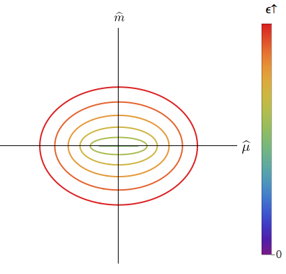
The position of the critical manifold resulting from these considerations is shown in Fig. 9 for both scenarios and in the continuum. The CP-violating phases lie within the (distorted) cone-shaped regions. The contour plots show how the circular contours of the continuum are distorted by discretization effects into ellipses. We note that, in the first-order scenario shown in Fig. 9c, if one passes through any point in the rectangular region in the $(\widehat{m},\epsilon)$ plane between the two critical lines there is a first-order transition at which the condensate changes discontinuously.

In this section we consider the effect on the previous results of the inclusion of the next highest order terms in our power counting, i.e. those scaling as $a^{3}\sim ma$. At this order we can still determine the vacuum using the classical potential of the chiral theory. The ${\cal O}(ma)$ term in this potential is standard, see, e.g. Ref. [25]. The ${\cal O}(a^{3})$ terms have been discussed for $\epsilon=0$ in Ref. [26]; the results carry over unchanged to $\epsilon\neq 0$ since the first additional term involving $\epsilon$ scales as $a\epsilon^{2}$ and is of higher order in our power-counting. The relevant additional terms entering the potential are

where $w$ and $w_{3}$ are new LECs. There is also a term proportional to $\tr(A^{\dagger}A)\tr(A^{\dagger}\Sigma+\Sigma^{\dagger}A)$, but this can removed by (yet another) redefinition of $\chi$. Inserting our standard parametrization $\left<\Sigma\right>=\exp(i\theta\vec{n}\cdot\vec{\tau})$, and combining the results with that from the LO potential, we obtain

The new LECs should satisfy $|w|\ll 1$ and $|w_{3}|\ll|w^{\prime}|,|c_{\ell}\epsilon^{2}|$ in order to be consistent with our power counting.

We begin by considering the untwisted theory, $\widehat{\mu}=0$, where the phase diagram and pion masses can be determined analytically. In this case $\widehat{m}=\chi_{\ell}$. As previously, the potential is minimized with $n_{3}=1$, so that

References

- [1] R. F. Dashen, Phys.Rev. D3, 1879 (1971).
- [2] M. Creutz, Phys.Rev.Lett. 92, 201601 (2004), arXiv:hep-lat/0312018 .
- [3] J. Beringer et al. (Particle Data Group), Phys.Rev. D86, 010001 (2012).
- [4] S. Aoki, Y. Aoki, C. Bernard, T. Blum, G. Colangelo, et al., Eur.Phys.J. C74, 2890 (2014), arXiv:1310.8555 [hep-lat] .
- [5] S. Aoki, Phys.Rev. D30, 2653 (1984).
- [6] S. R. Sharpe and J. Singleton, Robert L., Phys.Rev. D58, 074501 (1998), arXiv:hep-lat/9804028 .
- [7] S. Borsanyi, S. Durr, Z. Fodor, C. Hoelbling, S. Katz, et al., arXiv:1406.4088 [hep-lat] .
- [8] M. Creutz, (private communications and seminars) (2013).
- [9] R. Frezzotti and G. Rossi, JHEP 0408, 007 (2004a), arXiv:hep-lat/0306014 .
- [10] A. V. Smilga, Phys.Rev. D59, 114021 (1999), arXiv:hep-ph/9805214 .
- [11] S. Aoki and M. Creutz, Phys.Rev.Lett. 112, 141603 (2014), arXiv:1402.1837 [hep-lat] .
- [12] J. Gasser and H. Leutwyler, Nucl.Phys. B250, 465 (1985).
- [13] S. R. Sharpe and J. M. Wu, Phys.Rev. D70, 094029 (2004), arXiv:hep-lat/0407025 .
- [14] A. Walker-Loud and J. M. Wu, Phys.Rev. D72, 014506 (2005), arXiv:hep-lat/0504001 .
- [15] R. Frezzotti, P. A. Grassi, S. Sint, and P. Weisz (Alpha collaboration), JHEP 0108, 058 (2001), arXiv:hep-lat/0101001 .
- [16] A. Abdel-Rehim, P. Boucaud, N. Carrasco, A. Deuzeman, P. Dimopoulos, et al., PoS LATTICE2013, 264 (2013), arXiv:1311.4522 [hep-lat] .
- [17] N. Carrasco et al. (European Twisted Mass Collaboration), Nucl.Phys. B887, 19 (2014), arXiv:1403.4504 [hep-lat] .
- [18] G. de Divitiis et al. (RM123 Collaboration), Phys.Rev. D87, 114505 (2013), arXiv:1303.4896 [hep-lat] .
- [19] R. Frezzotti and G. Rossi, Nucl.Phys.Proc.Suppl. 128, 193 (2004b), arXiv:hep-lat/0311008 .
- [20] D. P. Horkel and S. R. Sharpe, (in preparation) .
- [21] G. Munster, JHEP 0409, 035 (2004), arXiv:hep-lat/0407006 .
- [22] L. Scorzato, Eur.Phys.J. C37, 445 (2004), arXiv:hep-lat/0407023 .
- [23] S. R. Sharpe and J. M. Wu, Phys.Rev. D71, 074501 (2005), arXiv:hep-lat/0411021 .
- [24] G. Munster and T. Sudmann, JHEP 0608, 085 (2006), arXiv:hep-lat/0603019 .
- [25] G. Rupak and N. Shoresh, Phys.Rev. D66, 054503 (2002), arXiv:hep-lat/0201019 .
- [26] S. R. Sharpe, Phys.Rev. D72, 074510 (2005), arXiv:hep-lat/0509009 .
- [27] M. Kieberg, K. Splittorff, J. Verbaarschot, and S. Zafeiropoulos, (talk at Lattice 2014) .
- [28] M. Golterman and Y. Shamir, Phys.Rev. D89, 054501 (2014), arXiv:1401.0356 [hep-lat] .