Time-dependent, compositionally driven convection in the oceans of accreting neutron stars
Abstract
We discuss the effect of chemical separation as matter freezes at the base of the ocean of an accreting neutron star, and the subsequent enrichment of the ocean in light elements and inward transport of heat through convective mixing. We extend the steady-state results of [38] to transiently accreting neutron stars, by considering the time-dependent cases of heating during accretion outbursts and cooling during quiescence. Convective mixing is extremely efficient, flattening the composition profile in about one convective turnover time (weeks to months at the base of the ocean). During accretion outbursts, inward heat transport has only a small effect on the temperature profile in the outer layers until the ocean is strongly enriched in light elements, a process that takes hundreds of years to complete. During quiescence, however, inward heat transport rapidly cools the outer layers of the ocean while keeping the inner layers hot. We find that this leads to a sharp drop in surface emission at around a week followed by a gradual recovery as cooling becomes dominated by the crust. Such a dip should be observable in the light curves of these neutron star transients, if enough data is taken at a few days to a month after the end of accretion. If such a dip is definitively observed, it will provide strong constraints on the chemical composition of the ocean and outer crust.
Subject headings
dense matter — stars: neutron — X-rays: binaries — X-rays: individualI. Introduction
The outermost m of an accreting neutron star is expected to form a fluid ocean that overlies the kilometer-thick solid crust of the star [3]. This ocean is of interest as the site of long duration thermonuclear flashes such as superbursts [13, 51, 33] and intermediate duration bursts [27, 14], non-radial oscillations [3, 41] and because the matter in the ocean eventually solidifies as it is compressed to higher densities by ongoing accretion, and so determines the thermal, mechanical and compositional properties of the neutron star crust [22, 5, 44]. The thermal properties of the ocean determine the initial cooling of an accreting neutron star following the onset of quiescence [7, hereafter BC09] as observed for 6 sources [54, 52, 55, 53, 9, 35, 10, 20, 16, 17, 19, 8].
The composition of the ocean is expected to consist of mostly heavy elements, formed by rapid proton capture (the rp-process) during nuclear burning of the accreted hydrogen and helium at low densities and subsequent electron captures at higher densities, although some carbon may also be present [45, 21]. At the ocean-crust boundary, as the matter transitions from liquid to solid it also undergoes chemical separation. Numerical simulations of phase transitions in neutron stars [24] have shown that as the ocean mixture solidifies, the lighter elements (charge numbers ) are preferentially left behind in the liquid whereas the heavier elements are preferentially incorporated into the solid. In Medin & Cumming [38] (hereafter Paper I), we showed that the retention of light elements in the liquid acts as a source of buoyancy that drives a continual mixing of the ocean, enriching it substantially in light elements and leading to a relatively uniform composition with depth. Heat is also transported inward to the ocean-crust boundary by this convective mixing. In Medin & Cumming [39] (hereafter Paper II) we showed that during quiescence the inward heat transport is particularly strong, leading to rapid cooling of the outer ocean and a significant drop in the light curve compared with standard cooling models (e.g., BC09).
One motivation for studying the problem of “compositionally driven” convection in the neutron star ocean comes from superbursts, which are thought to involve thermally unstable carbon burning in the deep ocean of the neutron star [13, 51]. The energy release in these very long duration thermonuclear flashes, inferred from fitting their light curves [14], corresponds to carbon fractions of . This has been challenging to produce in models of the nuclear burning of the accreted hydrogen and helium. If the hydrogen and helium burn unstably, the amount of carbon produced is [57], and whereas stable burning can produce large carbon fractions [46, 48], time-dependent models do not show stable burning at the Eddington accretion rates of superburst sources [28, although observationally, superburst sources show evidence that much of the accreted material may not burn in Type I bursts;]. Perhaps even more problematic than making enough carbon is that carbon ignition models for superbursts require large ocean temperatures at the ignition depth, which are difficult to achieve in standard models of crust heating [4, 14, 29, e.g.,].
Observations of quiescent transiently accreting neutron stars also provide strong motivation for studying ocean convection. BC09 inferred a large inward heat flux in the outer crust of the sources MXB 1659–29 and KS 1731–260 by fitting their light curves in quiescence. Other anomalous behavior from transiently accreting neutron stars includes a rebrightening during a cooling episode in XTE J1701–462 [20], and very rapid cooling a few days after accretion shut off in XTE J1709–267 [19]. Though both the rebrightening and the rapid cooling can be explained by a spurt of accretion during quiescence, as we show here these features may naturally arise from the cooling ocean when chemical separation occurs.
In this paper we generalize and expand on the results of Papers I and II: We place the steady-state calculations of Paper I in a larger context by adding the relevant physics into a full envelope-ocean-crust model (cf. Brown 4; BC09; Paper II) and by considering the evolution toward that steady state; and we examine the quiescence calculations of Paper II in greater detail and provide cooling curve fits for several additional sources. We begin in Section II by reviewing the picture of steady-state, compositionally driven convection as presented in Paper I, and discuss how the picture changes when time dependence is considered. In Section III we describe our calculation of the time-dependent temperature and composition structure of the ocean and crust. In Sections IV and V we present results from our calculation during accretion and during cooling after accretion turns off, respectively; in Section V.1 we additionally provide an analytic approximation to our cooling model. In Section VI we compare the cooling light curves we generate to observations of transiently accreting neutron stars during quiescence. Finally, in Section VII we discuss the implications of our results.
II. Compositionally driven convection in the ocean
II.1. Phase diagrams and chemical separation
As in Paper I, to understand the effect of compositionally driven convection on the ocean we first consider the phase diagram for the ocean mixture. Though the ocean in an accreting neutron star is likely made up of a wide variety of elements [45, 21], for computational tractability we only consider a two-component mixture of oxygen and selenium in this paper. Our O-Se mixture is modeled after the 17-component, rp-process ash mixture considered by [24] [21, see also]; in that latter mixture selenium is the most abundant element and oxygen is the most abundant low- element. While the relative abundances and mass numbers of each element change with depth due to electron captures, we ignore any such effects and use 16O-79Se throughout the ocean. It is unclear whether including two components is enough to accurately model the effects of chemical and phase separation in the ocean, and if so, what the charge values of those two components should be. Calculations of multicomponent phase diagrams using both extrapolation [37, cf.] and molecular dynamics techniques [25, e.g.,] are in progress to address these issues. Note that the equations in the body of the paper are specific to two-component mixtures, but that unless otherwise specified the equations in the Appendix are applicable generally to multicomponent mixtures.
The Coulomb coupling parameter is an important quantity for determining the phase diagram of two-component mixtures. The Coulomb coupling parameter for ion species is
| (1) |
while that for the mixture is
| (2) |
Here and are the ion charge and mass number, is the electron fraction, the density, and the temperature; signifies the number average of quantity for the mixture, such that , where is the number fraction of species .


Figure 1 shows two phase diagrams for a two-component mixture with charge ratio , appropriate for, e.g., an oxygen-selenium mixture (charge ratio ). The top panel shows the detailed phase diagram calculated in [37]; the bottom panel shows the approximate phase diagram used in the calculations in this paper. In each panel, the x-axis shows , the number fraction of the heavier ion species, and the left y-axis shows , the inverse of the Coulomb coupling parameter for the lighter species. For reference, the right y-axis shows , the inverse of the coupling parameter for the heavier species. In addition, “L” denotes the stable liquid region, “S1” and “S2” denote stable solid regions, and the shaded region represents the unstable region of the phase diagram. A parcel with composition and temperature (or equivalently, and ) that lies inside the unstable region will undergo phase separation, separating into two phases with compositions on either side of the unstable region.11 1 In the special case that is at its eutectic value, the parcel separates into three phases; for the example of Fig. 1, when , the parcel separates into L, S1, and S2. See Paper I. In this way, chemical separation occurs.
For a single species of ion, solidification occurs when [43, e.g.,]. For a multicomponent mixture a liquid becomes unstable to phase separation at a value that varies with composition, known as the liquidus curve (in Fig. 1, the upper boundary of the unstable region). For the charge mixture shown in Fig. 1 the liquidus curve is almost linear in vs. , with ; we have therefore chosen as the liquidus curve for our approximate phase diagram. Using Eq. (2) and the equation of state of relativistic, degenerate electrons (applicable for )
| (3) |
where is the column depth, is the pressure, and is the surface gravity, we have that the liquidus in our phase diagram corresponds to the column depth
| (4) |
where and are evaluated at the liquidus. Although a multicomponent liquid becomes unstable to phase separation at the liquidus, in general it does not completely solidify until a much larger value of . However, we found in Paper I that in the neutron star ocean any liquid-solid mixture formed during phase separation will differentiate spatially due to sedimentation of the solid particles at a rate much faster than any of the other mixing processes (including accretion driving).22 2 This requires the solid particles to be denser than the liquid, which for the phase diagram shown in Fig. 1 is true at all compositions except very close to unity. This means that all of the liquid in the ocean-crust region will lie above all of the solid there, such that the liquid effectively solidifies at the liquidus; the liquidus depth is also the depth of the ocean-crust boundary . In other words, from Eq. (4)
| (5) | ||||
| (6) |
where and are the temperature and ion charge at the base of the ocean.
II.2. Regimes of chemical separation
The fate of ocean-crust particles as they cross into the unstable region of the phase diagram and undergo phase/chemical separation is determined by the composition of the parcels before crossing and the direction they are moving on the diagram. The initial composition of the parcels depends on the accretion history of the neutron star. The direction each parcel moves on the phase diagram depends on whether accretion is ongoing or not; and if accretion is ongoing, whether the rate at which the ocean-crust boundary moves inward is greater than the rate at which particles are driven inward, i.e., whether , where is the rate of change in and is the local accretion rate per unit area. There are three regimes to consider: steady-state accretion, cooling after accretion shuts off, and rapid heating shortly after accretion turns on.
1) When the neutron star is accreting and the ocean-crust system is near or at its steady-state configuration, . In this regime accreted material is driven to higher pressure, such that material at the base of the ocean moves across the ocean-crust boundary and freezes (as shown by the arrow marked “driving” in Fig. 1). According to the simplified phase diagram in Fig. 1, if the ocean base has a composition or , there will be no chemical separation upon freezing. If , some material will remain liquid and some will form a solid of composition S2. If , some material will remain liquid and some will form a solid of composition S1.
2) When accretion turns off and the neutron star is cooling, and . In this regime the temperature drops in the ocean, such that the ocean-crust boundary moves outward and the base of the ocean freezes (“cooling” in Fig. 1). In this case the behavior of chemical separation with will be the same as that described above.
3) When accretion turns on again and the system moves toward its steady-state configuration, the heating is initially very strong. In this regime the crust melts faster than new material can be driven across the ocean-crust boundary, such that (and material follows the “heating” arrow in Fig. 1). According to our simplified phase diagram, if the crust has a composition , , or S2, there is no chemical separation of the solid upon melting. If the crust is of composition S1, there will be chemical and phase separation into a light liquid and an S2 solid. However, assuming diffusion between solid-solid phases is slow [26, cf.], as heating continues the liquid and the solid will travel together up the phase diagram until the solid melts and recombines with the liquid; since the distance over which this occurs is relatively short compared to the size of the ocean, we assume for simplicity that in our calculations a solid of composition S1 will just melt to form a liquid of composition S1 (). Therefore, in our calculations there is no chemical or phase separation when , regardless of crust composition.
II.3. Compositional buoyancy and convection
What happens to the liquid left behind after phase separation and sedimentation of the solid depends on its composition. During rapid heating (regime 3 of the previous subsection) the liquid remains in place at the base of the ocean, since it is heavier than or at the same composition as the liquid above it. During steady-state accretion or cooling (regimes 1 and 2), however, after the solid particles form and sediment out the liquid left behind is lighter than the liquid immediately above it and so will have a tendency to buoyantly rise. This is counteracted by the thermal profile, which is stably stratified in the absence of a composition gradient such that a rising fluid element will be colder than its surroundings and will tend to sink back down.
A measure of the buoyancy is the convective (Schwarzschild) discriminant , which is related to the Brunt-Väisälä frequency [12]. In Appendix A we derive the equations for convective stability; for a two-component mixture we can write [Eq. (A7); see also Kippenhahn & Weigert 30]
| (7) |
Here,
| (8) |
is the mass fraction of species , is the electron fraction of species , is the scale height, and and are the temperature and composition gradients. The adiabatic temperature gradient is taken at constant (specific) entropy and composition : . For a quantity , with the other independent thermodynamic variables held constant. Although neither nor are independent variables, being subject to the constraints and , here we treat them as such in order to show explicitly the ion and electron contributions to various expressions in this paper (e.g., the specific heat given below). The ion and electron contributions are then combined in Eqs. (8) and (16). Note that , , and are all positive quantities. If or the ocean is stable to convection. For example, if the composition is uniform so that , stability to convection requires the familiar condition . The maximum value of such that the ocean is stable to convection is therefore .
As steady-state accretion or cooling continues, light elements are continually deposited at the base of the ocean and must be transported upwards by convection. For efficient convection adjusts to be close to but slightly greater than zero. In Paper I we found that convection is extremely efficient throughout the ocean during steady-state accretion; in Appendix B of this paper we demonstrate that convection in the ocean is extremely efficient even during time-dependent heating or cooling, and even when effects due to rapid rotation () and moderate magnetic fields ( G) are considered. We therefore assume in the main body of the paper that
| (9) |
where convection is active (i.e., across the ocean convection zone).
II.4. Convection equations
Here we assume Newtonian physics, plane-parallel geometry, mixing length theory, and efficient convection [Eq. (9)]. In mixing length theory the value of the mixing length is highly uncertain; but note below that under the efficient convection assumption this parameter does not appear in our equations. The continuity equation for the flow of species is given by
| (10) |
where is the composition flux for species and is the sum of all composition sources. The entropy balance equation is given by [5, e.g.,]
| (11) |
where
| (12) |
is the total flux,
| (13) |
is the conductive heat flux, is the convective heat flux, is the thermal conductivity, and is the sum of all heat sources. The terms on the left-hand side of Eq. (11) can be written [Eqs. (A14) and (A13)]
| (14) |
and
| (15) |
where is the specific heat capacity,
| (16) |
, and . With the assumption of efficient convection, the convective heat flux in the ocean becomes [Eq. (B8)]
| (17) |
the entropy balance equation in the ocean becomes [Eq. (B10)]
| (18) |
and the entropy advection term in the ocean becomes
| (19) |
The steady-state versions of the above equations are similar to the convection equations from Paper I. Using Eq. (17) with the steady-state composition flux [Paper I or Eq. (34)], we have that the steady-state convective flux is given by
| (20) |
This equation differs from equation 43 of Paper I (which is in error) by the factor , which is less than in any part of the ocean; the extra factor does not qualitatively change the results of our earlier paper. In the deep ocean, because , , , , and have only a weak dependence on but , we also have that
| (21) |
(cf. the result during cooling, ; see Paper II) and
| (22) |
Since , we have from Eqs. (19) and (22) that . Therefore, using Eq. (11) we have that
| (23) |
in steady state, as we assumed in Paper I.
III. A model of the envelope, crust, and ocean in the time-dependent case
In our model we place the top of the envelope at (i.e., at the surface) and the base of the crust at . The envelope structure is found as in Brown et al. 6 [42, see also]. We assume an composition throughout the envelope. The crust structure and composition is found as in BC09, except that we leave the core temperature as a free parameter rather than solving for it self-consistently, and use Newtonian physics with a surface gravity constant across the envelope, ocean, and crust. General relativistic corrections are included only as an overall redshift of the time, , and effective temperature, , from the local value to that seen by an observer at infinity; here the neutron star mass and radius are 1.62 and 11.2 km, giving a redshift factor of . Note that while varies by about ten percent across the crust of a neutron star, it varies by less than a percent across the ocean, such that the assumption of constant will modify the crust structure somewhat but will have very little effect on the ocean structure (for a given heat flux coming from the crust). As in BC09, we characterize the thermal conductivity in the inner crust with a single number, the impurity parameter . Our treatment of in the crust, as well as our treatment of across all layers, is described in Appendix C. In the ocean the components of are found from the thermodynamic equations of Appendix D; , , and the other thermodynamic derivatives are found as in Paper I (see, e.g., equation 39 of that paper).
The ocean is bounded from above by the hydrogen and helium burning layer, which ends at a column depth . Rather than tracking the physics of this layer, we leave as a free parameter; in Sections IV and V we choose (e.g., Bildsten & Brown 2; cf. Fig. 2). The mass fraction of species at the top of the ocean, , is determined by the nuclear reactions within the burning layer [45, see]. For the 16O-79Se mixture described in Section II we nominally choose , as in Paper I (but see below). This is approximately the mixture the ocean would have if all of the light elements () were oxygen and all of the heavy elements () were selenium; further calculations, involving mixtures of more than two components, are required to determine whether this is a reasonable approximation.
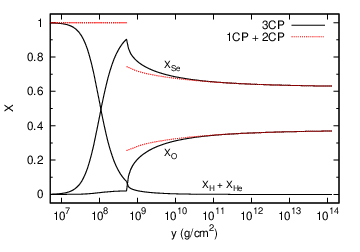
The heavy-element ocean cannot penetrate into the light-element burning layer, such that the burning layer is stable to convection and the convective velocity drops to zero at the boundary [Eq. (B2)]. To include the stabilizing effect of this layer in our model we set
| (24) |
and
| (25) |
The boundary conditions Eqs. (24) and (25) can occasionally be inconsistent with our assumption above, in which case we allow to grow as necessary. Figure 2 shows an example of a case where for our model (see also figure 3 from Paper II). Note that in the more accurate three-component model of Paper I there is no inconsistency between and , because the required rapid rise in with increasing column depth is stabilized by the rapid drop in . A similar situation occurs when convection is thermally driven ( and ) at the top of the ocean.
The ocean is bounded from below by the crust, which begins at a column depth . The mass fraction of species at the top of the crust, , is determined by the mass fraction of species at the base of the ocean, , according to the relevant phase diagram. For 16O-79Se we use Fig. 1 (see also Section II.2); converting from number fraction to mass fraction gives
| (26) |
for , and
| (27) |
for .
Convection can not occur for , since the region is solid; therefore, at the ocean-crust boundary we set
| (28) |
where the superscript ‘’ signifies that the flux is evaluated on the deep (i.e., crust) side of the boundary. The composition flux at the ocean base is
| (29) |
where and the superscript ‘’ signifies that the flux is evaluated on the shallow (i.e., ocean) side of the boundary [cf. the steady-state accretion expression of Paper I]. If , there will be no chemical separation at the boundary (Section II.2) and therefore no compositionally driven convection in the ocean, such that
| (30) |
and
| (31) |
throughout the ocean. Note that from Eqs. (26) and (29), for the O-Se system; with Eq. (17) this means that or that there is an inward heat flux at the base of the ocean due to compositionally driven convection (cf. Paper I).
We use a stationary grid for all column depths except , which we track continuously. The rate at which the ocean-crust boundary moves is constrained by the heat flux continuity condition
| (32) |
which using Eqs. (17) and (29) becomes
| (33) |
To estimate and we use the temperature gradient between and the nearest grid point on the low- side and on the high- side, respectively; for sufficiently small grid spacing this is a reasonable approximation. During rapid heating this approximation gives or , such that to maintain self-consistency between Eqs. (31) and (32) we can not use Eq. (33) to find but must find from Eq. (6).
In this paper we assume for simplicity that in the ocean. In particular, this means that we ignore the effect of electron captures on the ocean composition. Therefore, using Eqs. (10) and (24), the composition flux at any point in the ocean satisfies
| (34) |
From Eqs. (29) and (34) we have that the total change in ocean composition with time is given by
| (35) |
with ; this expression is used as a consistency check when we solve for below. The first term in Eq. (35) represents the balance between the composition entering the ocean from the burning layer and the composition leaving the ocean to the crust, as driven by accretion; the second term represents the exchange of particles in the ocean to convert a solid block of composition into a liquid block of composition , as the boundary moves inward (or vice versa as the boundary moves outward).
For the two-component ocean mixture considered in this paper, we solve for the evolution of the ocean composition and temperature structure as follows: In each time step we first guess a value for . Our guess comes from the fact that composition changes slowly with depth near the base of the ocean, i.e., ; which with Eq. (35) gives the approximation
| (36) |
where is obtained from Eq. (33). Once is chosen, the update value is found from
| (37) |
where is the current time step; at every other depth in the ocean is found from and Eq. (9), and then Eq. (37) is used to find at each depth. Finally, Eq. (34) is used with to find for Eq. (18). The value of is modified and the procedure repeated until Eq. (35) holds true. The new value of is found from , , and Eq. (6). We find that our initial guess, Eq. (36), often requires no extra iterations for reasonable accuracy.
From Eq. (35), the steady-state is reached when and ; that is, when the ocean-crust boundary stops moving and, if accretion is ongoing, when the composition at the top of the ocean is the same as that at the top of the crust (cf. Paper I). The latter condition happens in our 16O-79Se simulations when [see Eq. (26)] through a simple feedback mechanism: if at the ocean base, (the crust has composition S2), such that and rises above 0.37; if , (the crust has composition S1), such that and drops below 0.37; the composition of the ocean base hovers around . In reality the eutectic nature of the phase diagram at will most likely cause the ocean base to solidify in vertically lamellar sheets of alternating S1, S2 composition [56, e.g.,].
IV. Convection during accretion
Here we evolve an example O-Se ocean from quiescence to steady state after accretion turns on, using the time-dependent equations of Sections II and III and assuming that compositionally driven convection is active. For this example (), K, , and . For our initial conditions at the start of accretion we choose throughout the crust and ocean and (i.e., “S2” in Fig. 1) throughout the ocean. The latter assumption is made because, even though can be large after a cooling episode, during the initial heating there is rapid inward movement of the ocean-crust boundary but no chemical separation, such that the bulk of the ocean has the same composition as the accreted crust (Section II.2; but see Section VII).

Figure 3 shows the composition profile at various times during its evolution to steady state. The composition is shown only for the ocean; the top of the ocean is located at , while the base of the ocean is located at the rightmost extent of each curve and moves inward as increases. The top of the convection zone can also be seen in the figure, as the depth where reaches the burning layer level of 0.02 and flattens out.

Figure 4 shows the temperature profile at various times during its evolution to steady state. As is discussed in Section II.2, the ocean moves through two regimes to reach steady state: Initially there is no compositionally driven convection, because of the strong accretion heating such that ; the temperature profile reaches a quasi-steady state that matches the steady-state profile in the case without convection (the red dotted curve in Fig. 4) in only a few years. Once that quasi-steady state is reached, and the system slowly evolves over hundreds of years to the final steady state (the black solid curve with years).
While the ocean reaches the efficient convection state given by Eq. (9) relatively quickly, in approximately one convective turnover time (months to a few years; see Paper I), it takes much longer to reach steady state, as can be seen in Figs. 3 and 4. The time from the start of the accretion outburst to the start of steady state can be estimated from Eq. (36): for a steady-state composition at the base of the ocean (Section III), and a difference between the composition at the top of the ocean and the top of the crust [Eq. (26)], we have
| (38) |
(i.e., hundreds to thousands of years). Using Eq. (38) with , we find a steady-state time of years (cf. Fig. 3). Note that if we instead use , as is typical for low-mass X-ray binaries, years. If , as in the model of [24] for K, the time to reach steady state is still large: years. If the mass fraction of light elements entering the ocean is ten times larger (), however, as is the case for stable hydrogen and helium burning [48, e.g.,], is of order the accretion time.

Figure 5 shows the steady-state profiles for the total flux and the conduction and convection contributions. The convection contribution has a dependence, as in Eq. (21). At the top of the figure we have marked the locations of the three accretion heat sources considered in this paper: hydrogen and helium burning, electron captures, and pycnonuclear fusion (see Appendix C). Since in steady state [Eq. (23)], is constant outside of the heat source regions and drops by across each region. For example, electron captures are active from a column depth of to and release a total energy of [23, e.g.,], such that the total drop in over that range is .
Note that the results shown in Figs. 4 and 5 are qualitatively different from those in figure 6 of Paper I, despite the similarity in the parameters used. This is due to a simplification made in our earlier paper: , the outward radial heat flux coming from the crust, is not the same for a neutron star with compositionally driven convection as without. In reality, must be solved self-consistently with ; because is larger with convection, less heat flows into the ocean from the crust and therefore is smaller (or more negative, as is the case in Fig. 5), which limits the growth of [4, cf. figure 1 and discussion of]. For the example of Fig. 4 the steady-state temperature at (near the ocean crust-boundary) is only 4% larger with convection than without; whereas for the model of Paper I it is 20% larger. The inclusion of hydrogen and helium burning has a comparable impact on our model, increasing the temperature at by 5% (compare the blue dashed curve and the red dotted curve in Fig. 4).
V. Convection after accretion turns off
We now consider the evolution of the ocean as it cools in quiescence. We find that the evolution proceeds in four stages; these stages are discussed in detail in Paper II, but we outline them below for reference (cf. Figs. 6 and 7):
In stage 1, the base of the ocean has not yet started to cool and so the evolution is the same with or without convection. In stage 2, the cooling wave has reached the bottom of the ocean, and new crust begins to form, driving convection. Inward heat transport by convection rapidly cools the envelope and ocean but maintains the ocean-crust boundary at a nearly constant temperature and depth. The temperature gradient steepens with time. In stage 3, the temperature gradient at the base of the ocean reaches , the liquidus temperature gradient. The region around the ocean-crust boundary alternates between a state of strong convective heating and crust melting, and a state of suppressed convection due to the release of heavy elements into the ocean. The sporadic convection can no longer prevent the ocean base from cooling, and cooling returns to a level similar to during stage 1. In stage 4, the crust is thermally relaxed, the ocean cools too slowly for convection to support the steep gradient , and the temperature profile in the ocean flattens.
V.1. Analytic approximation
Here we present an analytic approximation to the model of Sections II and III applicable during cooling. In our approximation, we assume that the ocean thermal conductivity and the pressure scale height have the scaling relationships
| (39) |
respectively; these relationships are valid when the electrons are relativistic, i.e., for column depths around or greater than . For each stage of cooling (see above or Paper II), we use Eq. (39) and a flux equation [Eq. (43) or (50)] to solve for the temperature at depth ; and then solve for the effective temperature using the approximate relation (cf. BC09)
| (40) |
or equivalently,
| (41) |
where the superscript ‘(s)’ signifies that the quantity is evaluated at the beginning of stage of cooling. To solve for the evolution of we assume that the temperature profile through the ocean and crust has an initially constant gradient (cf. Fig. 4; see also below). During cooling, there is a transition between the thermally relaxed outer layers with constant outward heat flux , where is the Stefan-Boltzmann constant, and the inner layers still in steady state with outward heat flux [Eq. (13) with ]. While the cooling wave is still in the ocean, this transition is defined by the thermal time
| (42) |
[34, cf.]; the factor of two in Eq. (42) comes from integrating equation 7 of BC09 assuming Eq. (39) for and and that and are constant. We define the transition depth as the depth where the thermal time is equal to the cooling time .
During stage 1, the transition depth is above the base of the ocean, i.e., , and there is no compositionally driven convection. The transition from the steady-state heat flux for to the surface heat flux for is not sharp (see, e.g., the “20 days” curve of Fig. 6). For lack of a better model, and to maintain continuity between stages 1 and 2, we use a modified version of Eq. (50) for the heat flux: the (conductive) heat flux at any point is given by
| (43) |
Here signifies that the quantity is evaluated at depth . Equation (43) has the desired properties of being continuous and giving the correct heat flux values in the limiting cases and . With Eq. (39) we can solve Eq. (43) for the temperature profile through the ocean,
| (44) |
and the temperature at depth near the top of the ocean,
| (45) |
Here we assume and have defined
| (46) |
for convenience. From Eqs. (41) and (45) we obtain the scaling relation
| (47) |
In deriving Eq. (47) we grouped terms and used the fact that [Eq. (46)].
To determine and as a function of time during stage 1, we use Eq. (42):
| (48) |
and therefore
| (49) |
where is the time at the beginning of stage 2 (see below). Along with , , and [where is taken at the base of the ocean; Eq. (53)], Eqs. (48) and (49) can be inserted into Eq. (47) to solve for during stage 1 (cf. equation 8 of BC09).
During stages 2 and 3, the ocean is thermally relaxed, such that the flux through the ocean satisfies . Since [Paper I; see also Eq. (B8) with Eqs. (29) and (36)] and , we have that the conductive flux in the ocean is given by
| (50) |
Similar to our method for stage 1 above, we use Eq. (50) with Eq. (39) to solve for the temperature profile through the ocean,
| (51) |
and the temperature at depth near the top of the ocean,
| (52) |
where
| (53) |
and we assume that . From Eqs. (41) and (52) we obtain the scaling relation
| (54) |
In deriving Eq. (54) we grouped terms and used the fact that [Eq. (53)].
Stage 2 begins at a time , where is the thermal time evaluated at the base of the ocean. At the beginning of this stage the ocean base is still in steady state, . We assume that the transition depth is stationary, i.e., that and are constant. To determine as a function of time we look at the ocean energetics: The total energy stored in the ocean is
| (55) |
where is the surface area; using Eq. (51) and assuming that is constant in the ocean, that , and that and are small ( in this stage and typically), we have
| (56) |
As increases and the ocean cools, this energy is slowly depleted; using Eq. (56) and the fact that and are constant during stage 2, we have that the ocean energy changes at a rate
| (57) |
The depleted energy is released at the ocean base and must mask the cooling due to the difference between the flux entering the ocean from the crust and the flux leaving the ocean through the top; i.e.,
| (58) |
From Eq. (54) we have that
| (59) |
combining Eqs. (57)–(59) with gives
| (60) |
Along with and , Eq. (60) can be inserted into Eq. (54) to solve for during stage 2.
Stage 3 begins when , or at a time . We assume that is constant. To determine and as a function of time during stage 3, we use Eq. (42) with and at their solid values such that (BC09): Because conduction is very efficient at transporting heat in the crust, we assume that the temperature gradient in the crust from the ocean-crust boundary to the transition depth is flat (cf. Paper I); i.e., the ocean-crust boundary cools at the same rate as the transition depth, , or equivalently,
| (61) |
If enrichment is low, ) [Eq. (E10)], and we have
| (62) |
but if enrichment is high (as is the case in Fig. 6; see figure 3 of Paper II), , and we have
| (63) |
Along with , , and , Eqs. (61)–(63) can be inserted into Eq. (54) to solve for during stage 3.
V.2. Results
Here we evolve the O-Se ocean from Section IV as it cools after accretion turns off. For stages 1, 2, and 4 of cooling we use the equations from Sections II and III, with and as is appropriate during cooling. We can also use these equations for stage 3, but the resulting light curves are noisy unless the simulation time step and spatial resolution are very small, due to the quasi-periodic activation/deactivation of convection that occurs during this stage (see above). Instead, we use the following method, which has the advantage of requiring a much coarser time and spatial grid for (empirically) comparably smooth and accurate light curves: We assume that once compositionally driven convection is strong enough for , it will remain at that critical level as cooling continues; i.e., we assume that when ,
| (64) |
[cf. Eq. (32)]. Equation (33) can no longer be used to find , instead we use the ocean-crust boundary equations of Appendix E. From Eq. (E2) we have [cf. Eq. (6)]
| (65) |
where . We solve for using the entropy balance equation [Eq. (E7); cf. Eq. (11)]
| (66) | ||||
| (67) |
where is the grid spacing. Note that Eq. (67) drives the temperature gradient to . We solve for using the iteration method described earlier, except that our initial guess is [Eq. (E9)]
| (68) |
We use the above method whenever (i.e., during stage 3), for all of the calculations shown here and in Section VI. Note that even with this method, the light curves are slightly noisy in stage 3 (see, e.g., Fig. 7).
In this section we choose inital conditions at the start of cooling K near the base of the ocean, K at the base of the crust, and a constant temperature gradient in between; and at the base of the ocean with a composition profile given by Eq. (9) throughout the ocean. These are approximately the steady-state conditions from Section IV (see also BC09; Paper II). Note that our assumption of an initially constant temperature gradient in the ocean and crust means that the convective flux is zero at the start of cooling, which is not entirely consistent with the steady-state results of Section IV. Our intent here is to show the effects of compositionally driven convection on cooling only. In Section VI we run our simulations over an entire accretion cycle from outburst to quiescence, such that the convective fluxes during cooling are calculated in a self-consistent way.

Figure 6 shows the temperature profiles at various times during cooling, along with the analytic approximation to these profiles. As can be seen in the figure, the ocean-crust boundary moves outward more quickly during cooling than during accretion: Equation (33) as it applies to the cooling case is given by
| (69) |
using Eq. (13) with a temperature gradient at the ocean base (see below), we find . This is markedly different from the situation in Section IV, where over most of the evolution. The composition also evolves more quickly during cooling than during accretion: From Eq. (36) we have , which is a factor of times larger than the accretion value [cf. Eq. (38)].

Figure 7 shows the cooling light curve along with the analytic approximation. As can be seen in the figure, changing has a strong effect on the light curve. This is for two reasons: First, for a larger light-element fraction in the ocean the thermal conductivity is also larger; a larger reduces the temperature gradient in the ocean (while self-consistently increasing the flux there), which keeps the outer layers hotter both during steady-state accretion and at the end of cooling when the crust and core are equilibrated (see BC09). Second, for a larger light-element fraction in the ocean the ocean-crust boundary is deeper, which delays the onset of strong ocean cooling due to compositionally driven convection. Note that in Fig. 7 the analytic approximation deviates strongly from the model light curve for days. This is because our analytic expressions [Eqs. (47) and (54)] only account for cooling of the ocean and crust by heat conduction out through the envelope, not for late-time cooling by heat conduction into the core (cf. BC09).
VI. Comparison to observations
In Paper II we presented fits to observations of XTE J1701–462 and IGR J17480–2446, using our model of compositionally driven convection; here we present fits to observations of several additional quiescent, transiently accreting neutron stars. Our goal in making these fits was to understand qualitatively how including convection in the ocean changes the fitting parameters for these sources. Therefore, we did not attempt to accurately fit our model to the observational data using rigorous parameter searches. Similar to BC09, each source was fit by running our simulations from the onset of accretion through the duration of the accretion outburst, then turning off accretion and tracking the cooling light curve out to the end of the observation. In our fits we take and the duration of the accretion outburst from observations and fit to the parameters , , , and . Note that in [15] we assumed shallow heating in our fit of EXO 0748–676 (see also BC09). In this paper we do not include shallow heating in our model directly. Instead, we vary to provide the necessary shallow heating, with a larger placing the burning layer closer to the bulk of the ocean and heating it more.


Figures 8 and 9 (see also figure 4 of Paper II) show our fits to cooling light curves from several quiescent sources. Note that in most of our fits we use times larger than the standard value of (e.g., Bildsten & Brown 2; Paper I); i.e., we must invoke a significant shallow heat source. Convection does not directly reduce the required shallow heat source for each fit: For the same shallow heating (same values of ) the fits for our model with and without convection are generally equally valid (e.g., in Fig. 9); in addition, the fitted ocean temperature at the start of cooling is similar in both our model and that of BC09, implying the use of a comparable shallow heating model. Instead, convection justifies the use of larger values of in our models due to light-element enrichment, which in turn increases the thermal conductivity in the ocean and makes it hotter without the need for shallow heating (see, e.g., the effect of different values in Fig. 7).
In our fits here and in Paper II, several trends appear when comparing the light curve from the model with compositionally driven convection to that from the model without convection, for the same parameters (see also Fig. 7). First, at –100 days post-outburst the light curve with convection drops below the light curve without convection then flattens out, as the cooling transitions from stage 1 to stage 2 to stage 3 (Section V). This arises because the compositionally-driven convection transports heat inwards, rapidly cooling the ocean and temporarily slowing the cooling in the crustal layers where the phase separation occurs. Second, at late times the light curve with convection crosses above the light curve without convection, due to light-element enrichment during convection increasing the ocean thermal conductivity (stage 4); for several of our fits (IGR J17480–2446 from Paper II, EXO 0748–676, and MXB 1659–29) this happens within the observation. Third, our fits that have steep (shallow) light curves with convection will have correspondingly steep (shallow) light curves without convection; compare, e.g., our fits for MXB 1659–29 versus those for EXO 0748–676 in Fig. 9. This is because, whether or not compositionally driven convection is in effect, the crust ultimately drives the cooling (see Section V). We do not discuss the behavior of the crust cooling in this paper; a detailed discussion can be found in BC09.
As can be seen from Figs. 8 and 9, we generally fit currently available light curves equally well with and without compositionally driven convection. Detecting the signature of convection will require better sampling of the early phase of the cooling curve. XTE J1709–267 [19, with a 10 week outburst;] is the exception to the above generalization, since the model with convection fits better to the observed rapid decrease in the cooling light curve (Fig. 8; cf. stage 2 of Fig. 7). Convection also provides an explanation for the observed increase in the equilibrium flux level in IGR J17480–2446 from 2009 to 2014 (Degenaar et al. 18; see Paper II), because it allows the composition, and therefore the equilibrium temperature profile, to change from one accretion episode to the next. For XTE J1701–462 (Fridriksson et al. 20; see Paper II), we find that with convection we can match the drop in the light curve at – days (Fig. 10). Similarly for EXO 0748–676 [17, 15, with a 24 year outburst;], we find that the inclusion of convection leads to a plateau of slow cooling between –750 days post-outburst, broadly consistent with the data (Fig. 9). We note that the model with convection is not statistically preferred over the model without convection.
BC09 fit the light curve of MXB 1659–29 [55, 53, 10, 8, with a 2.5 year outburst;] with a standard cooling model. Using similar parameters and including convection gives a model light curve with a “stage 2” drop at days. Because of the gap in the data at –400 days, we have the freedom in our fits to choose where this drop occurs; we can instead move the drop to days by increasing to an unphysical 0.8 (but see below). Note that in our model there is an abrupt jump in the light curve at late time ( days in Fig. 9), where the base of the ocean is saturated with light elements and compositionally driven convection halts (Section V). This is a general feature of our fits to MXB 1659–29, as long as , and it arises due to the steep drop in the light curve which causes rapid and prolonged outward motion of the ocean-crust boundary and strong chemical separation (). The observations at late times neither support nor dispute the existence of this predicted bump (see Fig. 9).

With the model of Sections II and III it is impossible to fit both “anomalous” data points in the light curve of XTE J1701–462 (the two points from to days post-outburst in Fig. 10; see also figure 4 of Paper II). However, we can partially fit this data by considering ocean mixtures other than oxygen-selenium and/or large values of . Two such fits, one for a calcium-selenium ocean and one for an iron-selenium ocean [24, cf.], are shown in Fig. 10; here the light-element saturation in the ocean produces a bump in the light curve that matches the second anomalous data point and that has a peak occurring at the same time as the first anomalous data point. We believe these modifications to our basic model to be reasonable, considering our uncertainty regarding what two-component mixture to use for the ocean or whether a two-component mixture is an accurate representation of the ocean. The large changes produced in the light curves when different compositions are used (figure 4 of Paper II vs. Fig. 10) emphasizes the need for models with three or more components. In addition, as we discuss in Section VII, it may be possible to reproduce the amplitude of the rebrightening in XTE J1701–462 by including heating due to electron captures self-consistently in our convection model.
VII. Discussion
In this paper we have continued the exploration begun in Paper I of the consequences of chemical separation and subsequent compositionally driven convection in the ocean of accreting neutron stars; while the model described in Paper I included only a steady-state ocean, here we use a full envelope-ocean-crust model and track its behavior from the onset of accretion to the end of cooling.
We have discovered a strong effect due to compositionally driven convection on the light curves of cooling, transiently accreting neutron stars. As the neutron star cools after an accretion outburst, the ocean-crust boundary moves outward. We find that this leads to chemical separation, and then convective mixing and inward heat transport, in a manner similar to that during accretion but at a much faster rate. The inward heat transport cools the outer layers of the ocean rapidly, but keeps the inner layers hot; the result is a sharp drop in surface emission at around a week (depending on parameters), followed by a gradual recovery as the ocean base moves outward. Such a dip should be observable in the light curves of these neutron star transients, if enough data is taken at a few days to a month after the end of accretion. If such a dip is definitively observed, it will provide strong constraints on the chemical composition of the ocean and outer crust.
Enrichment of the ocean with carbon remains a major issue for superburst models [46]. Following Horowitz et al. [24] and Paper I, we chose oxygen as the light element for our examples in this paper, but we have calculated models with carbon as the light element with similar results (as expected, due to the comparable heavy-element-to-light-element charge ratios and mass numbers of the C-Se and O-Se systems which yield comparable phase diagrams and thermodynamic quantities). We find that chemical separation can enrich the ocean to the required carbon fraction [46] within a few months of cooling after an accretion outburst (cf. Section V). This is well within the estimated superburst recurrence time of 1–3 years [32, 28], and is far more efficient than either chemical separation during accretion heating or gravitational sedimentation during quiescence. The rapid enrichment during cooling may help explain the puzzling superburst observed immediately before the onset of an accretion outburst in EXO 1745–248 [1]: since the carbon in the ocean is at the required ignition level before accretion even starts, if the ocean can be heated strongly enough with a small amount of accretion a superburst can occur right at the beginning of an outburst.
In order for chemical separation to occur, however, the composition at the base of the ocean and at the top of the crust must differ; this will not happen if accretion outbursts are too short to push accreted material to the base of the ocean. Ultimately the carbon excess is being supplied by the ashes of the hydrogen and helium burning layer, with carbon mass fraction during unstable burning [57]. This excess is driven to the ignition depth within a few months to a year (); but it takes ten times longer to build the excess up to the required fraction 0.1 (cf. Fig. 3). The total build-up time is at best a factor of three longer than the estimated superburst recurrence time of 1–3 years [32, 28]. We suggest that while a recurrence rate of a few years can not be sustained through compositionally driven convection, it is possible to have several bursts in a row at that rate if a small fraction of carbon can be “stored” in the deep ocean or crust (perhaps in lamellar sheets; see Section III) after each burst. On the other hand, in ’t Zand et al. [28] inferred observationally that stable burning is happening in superburst sources. Although the physical mechanism for the stable burning is not understood, it could produce much larger carbon fractions [48], which would reduce the timescale needed to enrich the ocean even during accretion (Section IV).
Note that while compositionally driven convection may help superburst models reach the levels of carbon enrichment required for carbon ignition, it does not help the models reach the required large ocean temperatures K [14]. In fact, we find (Sections IV and V) that temperatures in the bulk of the ocean are slightly lower with convection than without.
Two issues presented in Paper I have been resolved in the Appendix of this paper. In Appendix B we discuss what happens when in the ocean (see also Section III). As we alluded to in Paper I, the small amount of hydrogen and helium in the transition region between the burning layer and the ocean stabilize the density gradient at the top of the ocean and allows for an unstable temperature gradient and heavy-element composition gradient simultaneously, such that there is no contradiction between a small convective velocity at the top of the ocean and a smooth composition transition from the burning layer to the ocean. In Appendix F we discuss how rotation and magnetic fields affect our model. We find that the efficient convection assumption Eq. (9) remains valid even in the presence of rapid rotation and moderate magnetic fields; the remaining temperature and composition evolution equations in the paper follow directly from it and are therefore also unaffected by rotation or magnetic field.
There remains much to be explored theoretically. We have included only two species in our calculations, oxygen and selenium, which approximates the rp-process ashes used by [24]. The phase diagram for multicomponent mixtures is complex but can be calculated [24, 37] and should be included. Multiple, consecutive, accretion outburst-quiescence cycles should also be simulated to obtain self-consistent composition profiles in the ocean and outer crust. It will be important to include carbon burning in the models.
We have assumed that solid particles form at a single depth. However, electron capture reactions may occur in the ocean (e.g., 56Fe captures at a density of ; Haensel & Zdunik 22), lowering the at that depth, and potentially leading to formation of solid particles pre-electron capture above the post-electron capture liquid layers. The heat released due to electron captures during mixing and sedimentation of the region could be observable in the light curve. Further work is needed to understand how electron captures would affect the model presented here.
Appendix A Convective stability
Here we derive expressions for the convective discriminant and other quantities related to entropy production and convective stability in the multicomponent oceans of neutron stars.
The usual stability requirement for a displaced fluid element is [30, e.g.,]
| (A1) |
where
| (A2) |
with the gradient in the star and the gradient felt by an element displaced at constant entropy and chemical composition (i.e., we assume the element is displaced with no radiated energy and no chemical diffusion). In the neutron star ocean, the sound speed is much larger than the convective velocity, such that a displaced element is always in pressure balance with its surroundings:
| (A3) |
Using Eq. (A3) and
| (A4) |
we can rewrite as
| (A5) |
defining
| (A6) |
and enforcing the constraints and , the convective discriminant becomes
| (A7) |
Appendix B Mixing length equations and efficient convection
Here we derive or define expressions for several quantities related to heat transfer and composition mixing, first using mixing length theory and then using the efficient convection assumption of Eq. (9). We discuss the the regimes in which either model is appropriate. Finally we discuss how to make these models consistent with an ocean that has .
In mixing length theory [30, e.g.,], a displaced element feels an average force per unit mass of
| (B1) |
applied over an average distance of ; assuming that approximately half of this work goes into the kinetic energy of the particle, the convective velocity is given by
| (B2) |
where is the sound speed and is the ratio between the convection mixing length and the scale height (but see Appendix F). The composition flux for species is given by
| (B3) |
where the composition “excess” of the displaced element over its surroundings is
| (B4) |
the convective heat flux is given by
| (B5) |
where
| (B6) |
using Eq. (A13). To solve for the evolution of the ocean using mixing length theory, we assume a value for and use Eqs. (B2)–(B6) to find and for Eqs. (10) and (11).
For efficient convection [Eq. (9)], Eq. (A13) becomes
| (B7) |
while Eq. (B5) with Eq. (B3) becomes
| (B8) |
Using Eqs. (10), (B7), and (B8) with , we have
| (B9) |
such that with Eqs. (12), (A14), and (B7) the energy balance equation Eq. (11) becomes
| (B10) |
To solve for the evolution of the ocean using the efficient convection assumption we use the procedure described in Section III. Note that Eqs. (B7)–(B10) are independent of , such that we do not need to assume a value for this parameter.
 |
 |
Figure 11 shows the composition profile for the example from Section IV, using mixing length theory with various values of , and using the efficient convection assumption. The value of at which efficient convection becomes a good approximation in the neutron star ocean can be estimated using Eq. (29) as an upper bound for the composition flux: Eq. (B3) gives
| (B11) |
using Eq. (B2), , and we have
| (B12) |
This means that for mixing length parameters (as we assumed in Paper I), convection is efficient; i.e., is extremely close to its maximum stable value, . Note that when , small numerical errors in lead to very large errors in . In this case we can not use the full mixing length procedure but must assume efficient convection.
In Paper I we suggested that a time-dependent calculation could help resolve what happens when a stable composition profile can not extend from the burning layer ash at the top of the ocean to the steady-state mixture at the ocean base (i.e., from to for the 16O-79Se system); this could happen, e.g., when at the top of the ocean. In the current paper we remove the inconsistency by allowing the composition at the top of the ocean to be different from that provided by the burning layer (e.g., Fig. 2; see also figure 3 from Paper II), and use the stabilizing effect of the burning layer on convection as justification. If we instead fix , we find that once the convection zone reaches the top of the ocean there is a flux at the outer boundary
| (B13) |
[Eqs. (10) and (29)], with because the system is not yet in steady state. In the O-Se system, this means that a large quantity of oxygen is being ejected from the ocean into the envelope, a fact that we are ignoring because of our assumption of a fixed envelope composition. We conclude that the only way to make our models consistent with a ocean is to consider the envelope, by either allowing ocean material to mix into the envelope [through Eq. (B13)], or by including hydrogen and helium burning in the envelope to prevent mixing (as in Fig. 2).
Appendix C Heat and composition sources
Here we derive expressions for the sources and , as used in the continuity equation Eq. (10) and entropy balance equation Eq. (11), respectively.
There are sources of composition change at three locations in our model:
1) At the ocean-crust boundary, composition changes abruptly due to chemical separation and rapid sedimentation of the solid at the phase transition. Formally, we write
| (C1) |
where is the Dirac delta function; but in practice we simply adjust manually without reference to Eq. (10).
2) At the hydrogen and helium burning layer, composition changes quickly due to the strong temperature dependence of the thermonuclear reactions, from in the envelope to at the top of the ocean. We assume that the burning layer is infinitely thin, such that formally we have
| (C2) |
Note that is not necessarily the value given by the burning layer ashes ( for the O-Se ocean model of this paper); we allow to vary based on the composition profile required by efficient convection in the ocean (see Section III).
3) In the crust, composition changes gradually due to electron captures and pycnonuclear fusion. For simplicity we set as the composition at the top of the crust, regardless of the value of , and follow the procedure of BC09 to obtain and at greater depths. With this approximation, only determines the physics of the liquid-solid phase transition [e.g., in Eq. (36)] and has no effect on the crust properties (thermal conductivity, etc.).
During accretion, there are heat sources at three locations in our model (see Fig. 5):
1) At the hydrogen and helium burning layer, particles are driven to a critical depth (temperature) for thermonuclear reactions by accretion; for these reactions release [5, e.g.,]. Following BC09, we assume that the heat is released uniformly in the logarithm of column depth, over a region from to , such that
| (C3) |
Here we choose and .
2) In the outer crust, electron captures release [23, e.g.,]; we use and .
2) In the inner crust, pycnonuclear fusion reactions release ; we use , and .
Appendix D Thermodynamic quantities
Here we derive or define expressions for several thermodynamic quantities in multicomponent plasmas that are used in this paper.
The total differential for the Gibbs free energy is given by
| (D1) |
where includes the energy of the ions and the electrons, is the total volume, is the total number of ion species in the plasma, is the chemical potential of ion species , is the number of ions of species , is the electron chemical potential, and is the number of electrons. Note that although for the fully-ionized multicomponent plasma, such that is not an independent thermodynamic variable, here we treat it as such in order to express the various relations derived in this section in terms of both ion and electron quantities. The ion and electron terms are combined in the rest of the paper [Eqs. (8) and (16)] to simplify the appearance of the equations. Using , , and the Euler integral
| (D2) |
where is the Gibbs free energy, we have
| (D3) |
Here is the “specific” version of the quantity ; i.e., , where is the total mass of the system and is the total number of ions. Using Eq. (D3) we can derive two useful Maxwell relations: Since
| (D4) |
we have
| (D5) |
similarly,
| (D6) |
We define
| (D7) |
and
| (D8) |
these terms are analogous to the ion and electron specific heat terms and for the composition. For degenerate electrons
| (D9) |
where is the Fermi energy with ; for the models we consider here the electrons are degenerate and Eq. (D9) holds throughout the ocean, since (for and K). An accurate expression for in the ocean can be obtained from and the free energy of a multicomponent liquid
| (D10) |
where (including the ideal gas part) is defined in equations 1 and 2 of [37]; we use this accurate expression in our numerical calculations. However, an approximation for can be obtained by considering only the ideal gas term, the dominant temperature-dependent term in :
| (D11) |
Appendix E Tracking the ocean-crust boundary
Here we derive expressions for the motion of the ocean-crust boundary, as well as the changes in entropy and composition at the ocean crust boundary.
Using Eq. (6) and
| (E1) |
we have that the ocean-crust boundary moves at a rate
| (E2) |
where
| (E3) |
and
| (E4) |
with
| (E5) |
and
| (E6) |
For an 16O-79Se mixture, . At the ocean-crust boundary, the energy balance equation Eq. (11) in the frame moving with the boundary is
| (E7) |
where indicates that the derivative is evaluated on the “downstream” side of the boundary: during heating (), and during cooling (). Note that and that during cooling.
Appendix F Effects of rotation and magnetic field on convection
The effects of rotation and magnetic fields on convection have been examined in many places (e.g., Stevenson 49, Stevenson 50, Jones 36, Christensen & Aubert 11; see also Showman, Kaspi, & Flierl 47). Here we use simple arguments to show that in the neutron star ocean, the efficient convection assumption Eq. (9) is very good even in the presence of rapid rotation () and moderate magnetic fields ( G).
We consider a two-component ocean mixture with a plane-parallel geometry and governed by Newtonian physics. We impose a gravitational field , rotation , and magnetic field , all uniform. We assume that during convective mixing, displaced fluid elements do not exchange heat or material with their surroundings until they have traveled a distance of order the mixing length ; but by rapidly contracting or expanding they maintain pressure balance with their surroundings (cf. Appendix A). We therefore have
| (F1) |
where and
| (F2) |
Note that the equations of Appendices D–B are unaffected by the inclusion of this magnetic “pressure” term because . In the rotating frame, the equation of motion for a fluid element displaced from its equilibrium position is
| (F3) |
where
| (F4) |
| (F5) |
is the buoyancy force (per unit volume) felt by the element,
| (F6) |
is the Coriolis force, and
| (F7) |
is the magnetic “tension” force. Here
| (F8) |
is the displacement of the element from its equilibrium position and
| (F9) |
is the perturbation to the magnetic field caused by this displacement. The magnetic tension term acts as a restoring force [31, cf.]: for a typical wavelength and a perpendicular field displacement of we have that
| (F10) |
such that
| (F11) |
where
| (F12) |
and
| (F13) |
is the Alfvén velocity.
We assume that the rotation and magnetic fields are oriented in no particular direction relative to each other or the gravitational field: and , where and . We then have the equations of motion
| (F14) |
and
| (F15) |
(with the assumptions made above, is independent of and , and so we do not consider it further). If we assume that both and depend on as , where is a constant, Eqs. (F14) and (F15) give
| (F16) |
Equations (B3) and (B5) for the composition and convective heat fluxes still apply when and , except that there is now the convective velocity only in the radial direction. Equation (B2) no longer applies, however, since the force per unit mass on the displaced element is not given by just the buoyancy term Eq. (B1). Instead we use
| (F17) |
The convective velocity must be large enough to carry the required composition flux Eq. (29); , the oscillation frequency for the convective instability, will grow until this happens. Comparing Eqs. (B3) and (29), we have that
| (F18) |
or assuming and (cf. Appendix B),
| (F19) |
For transiently accreting neutron stars and G, such that . Therefore we have from Eq. (F16) that
| (F20) |
and that
| (F21) |
From Eq. (F21) we see that , and therefore convection is inhibited, until the convective discriminant is at least as large as ; i.e., until the buoyancy force exceeds the magnetic tension force. A slight excess of over gives the composition flux necessary to transport the chemical imbalance at the base of the ocean.
Since while , we have
| (F22) |
i.e., the efficient convection assumption Eq. (9) is good even in the presence of rotation and magnetic fields.
Note that there is some ambiguity in the typical length scale for the problem. Putting Eq. (F21) back into Eqs. (F14) and (F15) gives
| (F23) |
since , the typical perturbation in the horizontal direction is much smaller than in the vertical direction. This may require an average displacement smaller than to be used in Eq. (F17) [49, see, e.g.,], which will increase the oscillation frequency required to generate the composition flux . However, we still have such that will not change much (unless also changes) and our conclusion remains the same. Note also that if the star is non-magnetic such that , Eq. (F16) instead gives
| (F24) |
and we have
| (F25) |
we again find that efficient convection is a good assumption.
References
- [1] Altamirano, D., Keek, L., Cumming, A. et al. 2012, MNRAS, 426, 927
- [2] Bildsten, L. & Brown, E. F. 1997, ApJ, 477, 897
- [3] Bildsten, L. & Cutler, C. 1995, ApJ, 449, 800
- [4] Brown, E. F. 2004, ApJ, 614, L57
- [5] Brown, E. F. & Bildsten, L. 1998, ApJ, 496, 915
- [6] Brown, E. F., Bildsten, L., & Chang, P. 2002, ApJ, 574, 920
- [7] Brown, E. F. & Cumming, A. 2009, ApJ, 698, 1020
- [8] Cackett, E. M., Brown, E. F., Cumming, A., Degenaar, N., Fridriksson, J. K., Homan, J., Miller, J. M., & Wijnands, R. 2013, ApJ, 774, 131
- [9] Cackett, E. M., Wijnands, R., Linares, M., Miller, J. M., Homan, J., & Lewin, W. H. G. 2006, MNRAS, 372, 479
- [10] Cackett, E. M., Wijnands, R., Miller, J. M., Brown, E. F., & Degenaar, N. 2008, ApJ, 687, L87
- [11] Christensen, U. R. & Aubert, J. 2006, Geophys. J. Int., 166, 97
- [12] Cox, J. P. 1980, Theory of Stellar Pulsation (Princeton: Princeton)
- [13] Cumming, A. & Bildsten, L. 2001, ApJ, 559, L127
- [14] Cumming, A., Macbeth, J., in ’t Zand, J. J. M., & Page, D. 2006, ApJ, 646, 429
- [15] Degenaar, N., Medin, Z., Cumming, A., et al. 2014, ApJ, submitted
- [16] Degenaar, N. & Wijnands, R. 2011, MNRAS, 412, 68
- [17] Degenaar, N., Wolff, M. T., Ray, P. S., et al. 2011, MNRAS, 412, 1409
- [18] Degenaar, N., Wijnands, R., Brown, E. F., et al. 2013a, ApJ, 775, 48
- [19] Degenaar, N., Wijnands, R., & Miller, J. M. 2013b, ApJ, 767, L31
- [20] Fridriksson, J. K., Homan, J., Wijnands, R., et al. 2011, ApJ, 736, 162
- [21] Gupta, S., Brown, E. F., Schatz, H., Möller, P., & Kratz, K.-L. 2007, ApJ, 662, 1188
- [22] Haensel, P. & Zdunik, J. L. 1990, A&A, 227, 431
- [23] Haensel, P. & Zdunik, J. L. 2008, A&A, 480, 459
- [24] Horowitz, C. J., Berry, D. K., & Brown, E. F. 2007, Phys. Rev. E, 75, 066101
- [25] Hughto, J., Horowitz, C. J., Schneider, A. S., Medin, Z., Cumming, A., & Berry, D. K. 2012, Phys. Rev. E, 86, 066413
- [26] Hughto, J., Schneider, A. S., Horowitz, C. J., & Berry, D. K. 2011, Phys. Rev. E, 84, 016401
- [27] in ’t Zand, J. J. M., Cumming, A., van der Sluys, M. V., Verbunt, F., & Pols, O. R. 2005, A&A, 441, 675
- [28] in ’t Zand, J. J. M., Kuulkers, E., Verbunt, F., Heise, J., & Cornelisse, R. 2003, A&A, 411, L487
- [29] Keek, L., in ’t Zand, J. J. M., Kuulkers, E., Cumming, A., Brown, E. F., & Suzuki, M. 2008, A&A, 479, 177
- [30] Kippenhahn, R. & Weigert, A. 1994, Stellar Structure and Evolution (Berlin: Springer)
- [31] Kulsrud, R. M. 2005, Plasma Physics for Astrophysics (Princeton: Princeton)
- [32] Kuulkers, E. 2002, A&A, 383, L5
- [33] Kuulkers, E., int ’t Zand, J. J. M., Homan, J., van Straaten, S., Altamirano, D., & van der Klis, M. 2004, in AIP Conf. Proc. 714, X-Ray Timing 2003: Rossi and Beyond, ed. P. Kaaret, F. K. Lamb, & J. H. Swank (Melville, NY: AIP), 257
- [34] Henyey, L. & L’Ecuyer, J. L. 1969, ApJ, 156, 549
- [35] Homan, J., van der Klis, M., Wijnands, R., et al. 2007, ApJ, 656, 420
- [36] Jones, C. A. 2000, Philos. Trans. R. Soc. A, 358, 873
- [37] Medin, Z. & Cumming, A. 2010, Phys. Rev. E, 81, 036107
- [38] Medin, Z. & Cumming, A. 2011, ApJ, 730, 97
- [39] Medin, Z. & Cumming, A. 2014, ApJ, 783, L3
- [40] Page, D. & Reddy, S. 2013, Phys. Rev. Lett., 111, 241102
- [41] Piro, A. L. & Bildsten, L. 2005, ApJ, 619, 1054
- [42] Potekhin, A. Y., Baiko, D. A., Haensel, P., & Yakovlev, D.G. 1999, A&A, 346, 345
- [43] Potekhin, A. Y. & Chabrier, G. 2000, Phys. Rev. E, 62, 8554
- [44] Schatz, H., Bildsten, L., Cumming, A., & Wiescher, M. 1999, ApJ, 524, 1014
- [45] Schatz, H., Aprahamian, A., Barnard, V., et al. 2001, Phys. Rev. Lett., 86, 3471
- [46] Schatz, H., Bildsten, L., Cumming, A., & Ouellette, M. 2003, Nucl. Phys. A, 718, 247
- [47] Showman, A. P., Kaspi, Y., & Flierl, G. R. 2011, Icar., 211, 1258
- [48] Stevens, J., Brown, E. F., Cumming, A., Cyburt, R., & Schatz, H. 2014, ApJ, 791, 106
- [49] Stevenson, D. J. 1979, Geophys. Astrophys. Fluid Dynam., 12, 139
- [50] Stevenson, D. J. 2003, Earth Planet. Sci. Lett., 208, 1
- [51] Strohmayer, T. E. & Brown, E. F. 2002, ApJ, 566, 1045
- [52] Wijnands, R., Guainazzi, M., van der Klis, M., & Méndez, M. 2002, ApJ, 573, L45
- [53] Wijnands, R., Homan, J., Miller, J. M., & Lewin, W. H. G. 2004, ApJ, 606, L61
- [54] Wijnands, R., Miller, J. M., Groot, P. J., Markwardt, C., Lewin, W. H. G., & van der Klis, M. 2001, ApJ, 560, L159
- [55] Wijnands, R., Nowak, M., Miller, J. M., Homan, J., Wachter, S., & Lewin, W. H. G. 2003, ApJ, 594, 952
- [56] Woodruff, D. P. 1973, The Solid-Liquid Interface (London: Cambridge)
- [57] Woosley, S. E., Heger, A., Cumming, A., et al. 2004, ApJS, 151, 75