Degree reduction of disk rational Bézier curves

Journal: Journal of LaTeX Templates

Mao Shi Address: School of Mathematics and Information Science of Shaanxi Normal University, Xi’an 710062, China Email: shimao@snnu.edu.cn

Abstract

How to quickly and stably realize the degree reduction of the rational Bézier curve is an open problem in CAGD. Based on the weighted least squares method and weighted sum method of multi-objective optimization, this paper transforms the degree reduction problem of the rational Bézier curve into a convex optimization problem and then uses quadratic programming to solve it. Prove that the solution is the minimum. Numerical experiments show that the method is fast and stable.

Keywords:

Disk rational Bézier curve, Degree reduction, Quadratic programming , Weighted least square , Weighted sum method

1 Introduction

For the stability and robustness of numerical operation, the interval algorithm was brought into the geometric design system. In 1992, Sederberg and Farouki [1] formally defined the interval Bézier curve. It can transfer a complete description of the approximate error along with the curve to other systems for the application. Thereafter, a series of practical algorithms such as curve/curve or surface/surface intersection, solid modeling, visualization stability, degree reduction, interval curve boundary problems, etc. were studied by [2, 3, 4, 5, 6]. However, interval curves have some drawbacks. That is, the interval generally enlarges rapidly in a computational process and the rectangular intervals are not rotationally symmetric [5]. However, Disk Bézier curves given by Lin and Rokne [7] can correct these shortcomings. On the other hand, because Bézier curves can’t represent conic precisely, Hu et al. [3][4] studied interval non-uniform rational B-splines (INURBS) curves and surfaces. In 2011, Based on parallel projection Shi [8] defined a disk rational Bézier curve, which differs from the classic disk rational Bézier in that its error radii are Bézier polynomial functions.

Degree reduction of parametric curves is another important problem in the geometric modeling system. It is useful in the data communication between the design system and data compression [9]. Compared with research on the degree reduction of the Bézier curve, the research on the degree reduction of the rational Bézier curve is less[5] [10]. Farin [11] described a degree reduction method for rational Bézier curves for interactive interpolation and approximation. Sederberg and Chang [12], Chen [13] and Sun et al.[14] achieved reduction through the approximate common divisor method. Qin and Guan [15] transformed the problem of approximating multi-degree reduction of rational curves and surfaces into quadratic programming. Cai and Wang [16] studied degree reduction of rational Bézier curves with the steepest descent method. Applying multi-objective optimization techniques, Shi [17] realized multi-degree reduction rational Bézier curves.

Each of the above methods has its pros and cons. Some lack robustness in floating-point environments [12] [13] [14]; some have slower calculation speeds [16], etc. Therefore, finding a simple and stable method to obtain the optimal degree reduction approximation of rational curves is still an open problem. In this paper, multi-objective optimization, weighted least squares, and quadratic programming are serve to dealing with degree reduction of disk rational Bézier curves. Compared with the previous methods, this method is simple and stable.

The paper has the following structure: In section 2, we review the definition and properties of disk rational Bézier curve in [8]. In section 3, we propose an efficient algorithm to the problem of degree reduction of rational disk Bézier curves. In section 4, bounding errors for degree reduction are analyzed, and some examples are provided.

2 Disk rational Bézier curves

2.1 Disk rational arithmetic

Let $\mathbb{R}$ and $\mathbb{R}^{+}$ denote the set of all real numbers and all nonnegative real numbers, respectively. A disk in the plane is defined as

(\textbf{q})=(x_{0},y_{0})_{r}=\{\textbf{x}\in\mathbb{R}^{2}\ |\ \|\textbf{x}-\textbf{q}\|\leq r,r\in\mathbb{R}^{+}\ \},

(1)

where q is the centric point and $r$ is the radius.

For $n$ disks $(\textbf{q}_{i})=(x_{i},y_{i})_{r_{i}}$ , we have the following linear combination [5] [7]

\displaystyle\sum_{i=0}^{n}k_{i}(\textbf{q}_{i})=\sum_{i=0}^{n}(k_{i}\textbf{q}_{i})=\left(\sum_{i=0}^{n}k_{i}x_{i},\sum_{i=0}^{n}k_{i}y_{i}\right)_{\sum\limits_{i=0}^{n}|k_{i}|r_{i}},\ k\in\mathbb{R}.

(2)

Similarly, the disk in three-dimensional space can be described as

\displaystyle\begin{split}(\textbf{P}^{\omega})&=(X_{0},Y_{0},\omega)_{r}=(\omega x_{0},\omega y_{0},\omega)_{r}\\ &=\{\textbf{x}^{\omega}=(\omega x,\omega y,\omega)\in\mathbb{R}^{3}\ |\ \|\textbf{{x}}^{\omega}-\textbf{P}^{\omega}\|\leq r\}.\end{split}

(3)

Applying the oblique projection $I(\cdot)$ to the disk $(\textbf{P}^{\omega})$ , we obtain a rational disk in the plane $\omega=1$

\displaystyle(\textbf{q})=I((\textbf{P}^{\omega}))=I(X_{0},Y_{0},\omega,r)=\left(\frac{X_{0}}{\omega},\frac{Y_{0}}{\omega}\right)_{r}=(x_{0},y_{0})_{r}.

(4)

2.2 Disk rational Bézier curves

On the basis of equations (2) and (4), a disk rational curve can be defined, whose radius function is a positive polynomial function, and its properties are the same as the disk Bézier one [8].
Definition 1. A disk rational Bézier curve of degree $n$ with control disk points $({\textbf{p}}_{i})=(x_{i},y_{i})_{r_{i}}$ and corresponding weights $\omega_{i}\in\mathbb{R}^{+},i=0,...,n,$ can be written as

\displaystyle\left(\mathbf{p}\right)\left(t\right)=\left(\textbf{p}\left(t\right);r\left(t\right)\right)=\left(\frac{\sum\limits_{i=0}^{n}{\textbf{p}_{i}}\omega_{i}B_{i}^{n}\left(t\right)}{\sum\limits_{i=0}^{n}{\omega_{i}}B_{i}^{n}\left(t\right)};\sum_{i=0}^{n}{r_{i}}B_{i}^{n}\left(t\right)\right),0\leq t\leq 1,

(5)

where $B_{i}^{n}(t)={n\choose i}t^{i}(1-t)^{n-i},i=0,...,n,$ are Bernstein polynomials, ${\textbf{p}}(t)$ and $r(t)$ are called the center curve and the radius of the disk rational Bézier curve $(\textbf{{p}})(t)$ , respectively.

Given another disk rational Bézier curves $(\check{{\textbf{p}}})(t)$ of degree $m$ $(m<n)$

\left({\check{\mathbf{p}}}\right)\left(t\right)=\left({\check{\mathbf{p}}}\left(t\right);\check{r}\left(t\right)\right)=\left(\frac{\sum\limits_{i=0}^{m}{{\check{\mathbf{p}}}_{i}}\check{\omega}_{i}B_{i}^{m}\left(t\right)}{\sum\limits_{i=0}^{m}{\check{\omega}_{i}}B_{i}^{m}\left(t\right)};\sum_{i=0}^{m}{\check{r}_{i}}B_{i}^{m}\left(t\right)\right),

(6)

if the following equations are satisfied

\displaystyle\begin{array}[]{cc}\sum\limits_{j=max(0,i-n)}^{min(m,i)}{{m\choose j}{n\choose i-j}}\check{\omega}_{j}\omega_{i-j}\left({\textbf{p}}_{i-j}-\check{{\textbf{p}}}_{j}\right)=\mathbf{0},\ i=0,1,...,n+m,\end{array}

\displaystyle r_{i}=\sum_{j=max(0,i-n+m)}^{min(m,i)}\frac{{m\choose j}{n-m\choose i-j}\check{r}_{j}}{{n\choose i}},\ \ i=0,1,\ldots,n,

(9)

we say that a degree $n$ disk rational Bézier curve $({\textbf{{p}}})(t)$ can be represented exactly by a degree $m$ disk rational Bézier curve $(\check{\textbf{{p}}})(t)$ .

However, in many cases, we must use approximation methods to achieve the degree reduction of the disk rational Bézier curve.

3 Degree reduction of disk rational Bézier curves

3.1 Description of approximation problem

The problem of degree reduction of disk Rational Béziers curve can be stated as follows:
Problem 1. Given a degree $n$ disk rational Bézier curve $(\textbf{{p}})(t)$ , find a degree $m<n$ disk rational Bézier curve $(\check{\textbf{{p}}})(t)$ such that $(\check{\textbf{{p}}})(t)$ is the closure of $(\textbf{{p}})(t)$ .

By the weighted sum method of multi-objective optimization [18], the above problem can be summarized as

		$\displaystyle(A)\ \min\ \ \frac{1}{2}\left(F_{x}+F_{y}\right)$			(10a)
		$\displaystyle\ \ \ \ \ s.t.\ \ \check{\omega_{i}}>0,i=0,...,m$
		$\displaystyle(B)\min\limits_{\check{r}(t)\geq r(t)+dist(\textbf{{p}}(t),{\check{\textbf{{p}}}}(t))}\\|\check{r}(t)-r(t)\\|,$			(10b)

where $dist(\textbf{{p}}(t),\check{\textbf{{p}}}(t)),t\in[0,1]$ is the Hausdorff distance between the curve $\check{{\textbf{p}}}(t)$ and the curve $\textbf{{p}}(t)$ , $\rho(t)>0$ is a weight function and

\left(F_{x},\ F_{y}\right)=\int_{0}^{1}{\rho\left(t\right)\left(\textbf{p}\left(t\right)-\check{\textbf{{p}}}\left(t\right)\right)^{2}dt}.

(11)

That is, the degree reduction of the disk rational bézier curve is composed of two parts, one is the degree reduction of the central curve $\check{{\textbf{p}}}(t)$ , and the other for the error radius curve $r(t)$ .

3.2 Degree reduction approximation of center curve

In order to ensure that all weights are positive, we give some basic theorems firstly and then use quadratic programming to achieve the degree reduction of the central curve.

Lemma 1.

[16] The rational Bézier curves $\check{\textbf{p}}(t)$ and $\textbf{p}(t)$ satisfy $C^{(u,v)}$ -continuity if and only if the following equations are true:

\sum_{i=0}^{q}{{n\choose{q-i}}{m\choose i}\omega_{q-i}\check{\omega}_{i}\check{\textbf{{p}}}_{i}}=\sum_{i=0}^{q}{{m\choose{q-i}}{n\choose i}\check{\omega}_{q-i}\omega_{i}\textbf{p}_{i}},\ q=0,\cdots,u;

(12)

and

		$\displaystyle\sum_{i=0}^{l}{{n\choose{n-i}}{m\choose m-l+i}\omega_{n-i}\check{\omega}_{m-l+i}\check{\textbf{{p}}}_{m-l+i}}=\sum_{i=0}^{l}{{m\choose{m-i}}{n\choose n-l+i}\check{\omega}_{m-i}\omega_{n-l+i}\textbf{p}_{n-l+i}},$
		$\displaystyle l=0,\cdots,v.$		(13)

Rewriting Lemma 1, we have

Theorem 1.

Any component of the vector $\mathbf{\check{P}}^{\mathbf{I}}=\left[\check{\omega}_{0}\mathbf{\check{p}}_{0},\cdots,\check{\omega}_{u}\mathbf{\check{p}}_{u}\right]^{\rm T}$ can be expressed as a linear combination of components in the vector $\bm{\check{\omega}}^{\mathbf{I}}=\left[\check{\omega}_{0},\cdots,\check{\omega}_{u}\right]^{\rm T}.$ It also holds for $\mathbf{\check{P}}^{\mathbf{III}}=\left[\check{\omega}_{m-v}\mathbf{\check{p}}_{m-v},\cdots,\check{\omega}_{m}\mathbf{\check{p}}_{m}\right]^{\rm T}$ and $\bm{\omega}^{\mathbf{III}}=\left[\check{\omega}_{m-v},\cdots,\check{\omega}_{m}\right]^{\rm T}.$ That is

\mathbf{\check{P}}^{\mathbf{I}}=\mathbf{S}_{1}^{-1}\mathbf{T}_{1}\bm{\check{\omega}}^{\mathbf{I}}

(14)

and

\mathbf{\check{P}}^{\mathbf{III}}=\mathbf{S}_{3}^{-1}\mathbf{T}_{3}\bm{\check{\omega}}^{\mathbf{III}},

(15)

where
$\mathbf{S}_{1}\!=\!\left[s^{1}_{ij}\right]\!=\!\left[{n\choose i-j}{m\choose j}\omega_{i-j}\right],\mathbf{T}_{1}\!=\!\left[t^{1}_{ij}\right]\!=\!\left[{n\choose i-j}{m\choose j}\omega_{i-j}\mathbf{p}_{i-j}\right],(0\leq j\leq i\leq u),$ $\mathbf{S}_{3}\!=\!\left[s^{3}_{kl}\right]\!=\!\left[{n\choose n+k-l}{m\choose m-v+l}\omega_{n+k-l}\right],\mathbf{T}_{3}\!=\!\left[t^{3}_{kl}\right]\!=\!\left[{n\choose n+k-l}{m\choose m-v+l}\omega_{n+k-l}\mathbf{p}_{n+k-l}\right],(0\leq k\leq l\leq v).$

Proof.

Equation (12) can be rewritten in matrix form

		$\displaystyle\left[\begin{smallmatrix}{n\choose 0}\omega_{0}&0&\cdots&0\\ {n\choose 1}\omega_{1}&{n\choose 0}\omega_{0}&\cdots&0\\ \vdots&\vdots&\ddots&\vdots\\ {n\choose u}\omega_{u}&{n\choose u-1}\omega_{u-1}&\cdots&{n\choose 0}\omega_{0}\\ \end{smallmatrix}\right]\left[\begin{smallmatrix}{m\choose 0}&0&\cdots&0\\ 0&{m\choose 1}&\cdots&0\\ \vdots&\vdots&\ddots&\vdots\\ 0&0&\cdots&{m\choose u}\\ \end{smallmatrix}\right]\left[\begin{smallmatrix}\check{\omega}_{0}\mathbf{\check{p}}_{0}\\ \check{\omega}_{1}\mathbf{\check{p}}_{1}\\ \vdots\\ \check{\omega}_{u}\mathbf{\check{p}}_{u}\\ \end{smallmatrix}\right]$
		$\displaystyle=\left[\begin{smallmatrix}{n\choose 0}\omega_{0}\mathbf{p}_{0}&0&\cdots&0\\ {n\choose 1}\omega_{1}\mathbf{p}_{1}&{n\choose 0}\omega_{0}\mathbf{p}_{0}&\cdots&0\\ \vdots&\vdots&\ddots&\vdots\\ {n\choose u}\omega_{u}\mathbf{p}_{u}&{n\choose u-1}\omega_{u-1}\mathbf{p}_{u-1}&\cdots&{n\choose 0}\omega_{0}\mathbf{p}_{0}\\ \end{smallmatrix}\right]\left[\begin{smallmatrix}{m\choose 0}&0&\cdots&0\\ 0&{m\choose 1}&\cdots&0\\ \vdots&\vdots&\ddots&\vdots\\ 0&0&\cdots&{m\choose u}\\ \end{smallmatrix}\right]\left[\begin{smallmatrix}\check{\omega}_{0}\\ \check{\omega}_{1}\\ \vdots\\ \check{\omega}_{u}\\ \end{smallmatrix}\right]$

Regrouping the above matrix equation, it yields

		$\displaystyle\left[\begin{smallmatrix}\check{\omega}_{0}\mathbf{\check{p}}_{0}\\ \check{\omega}_{1}\mathbf{\check{p}}_{1}\\ \vdots\\ \check{\omega}_{u}\mathbf{\check{p}}_{u}\\ \end{smallmatrix}\right]=\left[\begin{smallmatrix}{n\choose 0}{m\choose 0}\omega_{0}&0&\cdots&0\\ {n\choose 1}{m\choose 0}\omega_{1}&{n\choose 0}{m\choose 1}\omega_{0}&\cdots&0\\ \vdots&\vdots&\ddots&\vdots\\ {n\choose u}{m\choose 0}\omega_{u}&{n\choose u-1}{m\choose 1}\omega_{u-1}&\cdots&{n\choose 0}{m\choose u}\omega_{0}\\ \end{smallmatrix}\right]^{-1}$
		$\displaystyle\times\left[\begin{smallmatrix}{m\choose 0}{n\choose 0}\omega_{0}\mathbf{p}_{0}&0&\cdots&0\\ {n\choose 1}{m\choose 0}\omega_{1}\mathbf{p}_{1}&{n\choose 0}{m\choose 1}\omega_{0}\mathbf{p}_{0}&\cdots&0\\ \vdots&\vdots&\ddots&\vdots\\ {n\choose u}{m\choose 0}\omega_{u}\mathbf{p}_{u}&{n\choose u-1}{m\choose 1}\omega_{u-1}\mathbf{p}_{u-1}&\cdots&{n\choose 0}{m\choose u}\omega_{0}\mathbf{p}_{0}\\ \end{smallmatrix}\right]\left[\begin{smallmatrix}\check{\omega}_{0}\\ \check{\omega}_{1}\\ \vdots\\ \check{\omega}_{u}\\ \end{smallmatrix}\right],$

which establishes equation (12). Similarly, equation (15) also holds by (13).

Letting

\rho\left(t\right)=\left(\sum\limits_{i=0}^{m}{\check{\omega}_{i}B_{i}^{m}\left(t\right)}\sum\limits_{i=0}^{n}{\omega_{i}B_{i}^{n}\left(t\right)}\right)^{2}

(16)

and substituting $\mathbf{p}\left(t\right)$ and $\check{\bf{p}}\left(t\right)$ into equation (11), it yields

		$\displaystyle\left[F_{x}\left(t\right),F_{y}\left(t\right)\right]$
		$\displaystyle=\int_{0}^{1}{\left(\sum_{i=0}^{m}{\check{\omega}_{i}B_{i}^{m}\left(t\right)}\sum_{i=0}^{n}{\omega_{i}\mathbf{p}_{i}B_{i}^{n}\left(t\right)}-\sum_{i=0}^{m}{\check{\omega}_{i}\mathbf{\check{p}}_{i}B_{i}^{m}\left(t\right)\sum_{i=0}^{n}{\omega_{i}B_{i}^{n}\left(t\right)}}\right)^{2}dt}.$		(17)

When the above equation reaches its minimum, we must have

		$\displaystyle\frac{\partial\left(F_{x}\left(t\right),F_{y}\left(t\right)\right)}{\partial\mathbf{\check{p}}_{k}}\ \ \ \ (k=u+1,\ldots,m-v-1)$
		$\displaystyle\!=\!2\int_{0}^{1}{\left(\!\sum_{i=0}^{n}{\omega_{i}\mathbf{p}_{i}B_{i}^{n}\left(t\right)}\!\sum_{i=0}^{m}{\check{\omega}_{i}B_{i}^{m}\left(t\right)}\!-\!\sum_{i=0}^{n}{\omega_{i}B_{i}^{n}\left(t\right)}\sum_{i=0}^{m}{\check{\omega}_{i}\mathbf{\check{p}}_{i}B_{i}^{m}\left(t\right)}\right)\sum_{i=0}^{n}{\omega_{i}B_{i}^{n}\left(t\right)}}B_{k}^{m}\left(t\right)dt$
		$\displaystyle=\mathbf{0}$

Unfolding the above equation and writing it in matrix form, we deduce

\mathbf{S}_{2}\mathbf{\check{P}}^{\mathbf{II}}=\mathbf{D}\bm{\check{\omega}}-\mathbf{S}_{2}^{\mathbf{L}}\mathbf{\check{P}}^{\mathbf{I}}-\mathbf{S}_{2}^{\mathbf{R}}\mathbf{\check{P}}^{\mathbf{III}},

(18)

where $\mathbf{\check{P}}^{\mathbf{II}}=\left[\check{\omega}_{u+1}\mathbf{\check{p}}_{u+1},\cdots,\check{\omega}_{m-v-1}\mathbf{\check{p}}_{m-v-1}\right]^{\rm T},$ $\bm{\check{\omega}}=\left[\check{\omega}_{0},\cdots,\check{\omega}_{m}\right]^{\rm T},$

\mathbf{S}_{2}=\left[S_{ij}^{2}\right]=\left[{\sum\limits_{h=0}^{2n}{\frac{{{m\choose{u+i}}{2n\choose h}{m\choose{u+j}}A_{h}}}{{\left({2m+2n+1}\right){{2m+2n}\choose{2u+i+j+h}}}}}}\right],\ (i,j=1,\ldots,m-u-v-1),

\mathbf{D}=\left[D_{ij}\right]=\left[{\sum\limits_{h=0}^{2n}{\frac{{{m\choose{u+i}}{2n\choose h}{m\choose{j}}\mathbf{C}_{h}}}{{\left({2m+2n+1}\right){{2m+2n}\choose{u+i+j+h}}}}}}\right],\ (i=1,\ldots,m-u-v-1;j=0,\ldots,m),

\mathbf{S}_{2}^{\mathbf{L}}=\left[S_{ij}^{L}\right]=\left[{\sum\limits_{h=0}^{2n}{\frac{{{m\choose{u+i}}{2n\choose h}{m\choose{j}}A_{h}}}{{\left({2m+2n+1}\right){{2m+2n}\choose{u+i+j+h}}}}}}\right],\ (i=1,\ldots,m-u-v-1;j=0,\ldots,u),

\mathbf{S}_{2}^{\mathbf{R}}=\left[S_{ij}^{R}\right]=\left[{\sum\limits_{h=0}^{2n}{\frac{{{m\choose{u+i}}{2n\choose h}{m\choose{m-v+j}}A_{h}}}{{\left({2m+2n+1}\right){{2m+2n}\choose{m-v+u+i+j+h}}}}}}\right],\ (i=1,\ldots,m-u-v-1;j=0,\ldots,v),

$A_{i}=\sum\limits_{j=\max\left(0,i-n\right)}^{\min\left(n,i\right)}{\frac{{n\choose j}{n\choose i-j}}{{2n\choose i}}\omega_{j}\omega_{i-j}}$ and $\mathbf{C}_{i}=\sum\limits_{j=\max\left(0,i-n\right)}^{\min\left(n,i\right)}{\frac{{n\choose j}{n\choose i-j}}{{2n\choose i}}\omega_{j}\mathbf{p}_{j}\omega_{i-j}}.$

Substituting equations (14) and (15) into equation (18), we obtain

Theorem 2.

Under the action of the weighted least squares and $\rho\left(t\right)$ , any component of the vector $\mathbf{\check{P}}^{\mathbf{II}}$ is a linear combinations of components in the vector $\bm{\check{\omega}},$ and

	$\displaystyle\mathbf{\check{P}}^{\mathbf{II}}$	$\displaystyle=\mathbf{S}_{2}^{-1}\left(\mathbf{D}\bm{\check{\omega}}-\mathbf{S}_{2}^{\mathbf{L}}\mathbf{S}_{1}^{-1}\mathbf{T}_{1}\bm{\check{\omega}}^{\mathbf{I}}-\mathbf{S}_{2}^{\mathbf{R}}\mathbf{S}_{3}^{-1}\mathbf{T}_{3}\bm{\check{\omega}}^{\mathbf{III}}\right)$
		$\displaystyle=\mathbf{S}_{2}^{-1}\left(\mathbf{D}-\left[\begin{matrix}\mathbf{S}_{2}^{\mathbf{L}}\mathbf{S}_{1}^{-1}\mathbf{T}_{1}&\mathbf{0}_{\left(m-u-v-1\right)\times\left(m-u-v-1\right)}&\mathbf{S}_{2}^{\mathbf{R}}\mathbf{S}_{3}^{-1}\mathbf{T}_{3}\\ \end{matrix}\right]\right)\bm{\check{\omega}}.$		(19)

Finally, combining Theorems 1 and 2, it yields

Theorem 3.

$\mathbf{\check{P}}$ and $\bm{\check{\omega}}$ have the following relation

\mathbf{\check{P}}=\mathbf{Q}\bm{\check{\omega}},

(20)

where $\mathbf{\check{P}}=\left[\check{\omega}_{0}\mathbf{\check{p}}_{0},\cdots,\check{\omega}_{m}\mathbf{\check{p}}_{m}\right]^{\rm T}$ and

\mathbf{Q}=\left[\begin{array}[]{cc}\mathbf{S}_{1}^{-1}\mathbf{T}_{1}&\mathbf{0}_{\left(u+1\right)\times\left(m-u\right)}\\ \lx@intercol\hfil\mathbf{S}_{2}^{-1}\left(\mathbf{D}-\left[\begin{matrix}\mathbf{S}_{2}^{\mathbf{L}}\mathbf{S}_{1}^{-1}\mathbf{T}_{1}&\mathbf{0}_{\left(m-u-v-1\right)\times\left(m-u-v-1\right)}&\mathbf{S}_{2}^{\mathbf{R}}\mathbf{S}_{3}^{-1}\mathbf{T}_{3}\\ \end{matrix}\right]\right)\hfil\lx@intercol\\ \mathbf{0}_{\left(v+1\right)\times\left(m-v\right)}&\mathbf{S}_{3}^{-1}\mathbf{T}_{3}\\ \end{array}\right].

Using equation (20), equation (17) can be expressed as

\left[F_{x},F_{y}\right]=\bm{\check{\omega}}^{\rm T}\int_{0}^{1}{\left(\mathbf{P}^{\text{T}}\mathbf{K}-\bm{\omega}^{\rm T}\mathbf{KQ}\right)^{\rm T}\left(\mathbf{P}^{\text{T}}\mathbf{K}-\bm{\omega}^{\rm T}\mathbf{KQ}\right)dt}\bm{\check{\omega}},

(21)

where $\mathbf{P}=\left[\omega_{0}\bm{p}_{0},\cdots,\omega_{n}\bm{p}_{n}\right]^{\rm T},\ \bm{\omega}=\left[\omega_{0},\cdots,\omega_{n}\right]^{\rm T}$ and

\mathbf{K}=\left[\begin{matrix}B_{0}^{n}\left(t\right)B_{0}^{m}\left(t\right)&\cdots&B_{0}^{n}\left(t\right)B_{m}^{m}\left(t\right)\\ \vdots&\ddots&\vdots\\ B_{n}^{n}\left(t\right)B_{0}^{m}\left(t\right)&\cdots&B_{n}^{n}\left(t\right)B_{m}^{m}\left(t\right)\\ \end{matrix}\right].

Obviously, equation (21) is positive, so we have

Theorem 4.

The Hessian matrix of equation (17)

\left[H_{x},H_{y}\right]=\int_{0}^{1}{\left(\mathbf{P}^{\rm T}\mathbf{K}-\bm{\omega}^{\rm T}\mathbf{KQ}\right)^{\rm T}\left(\mathbf{P}^{\rm T}\mathbf{K}-\bm{\omega}^{\rm T}\mathbf{KQ}\right)dt}

(22)

is positive definite, and the solution of equation (10a) with respect to $\check{\omega}_{i},\ (i=0,\ldots,m)$ is unique.

Finally, $\bm{\check{\omega}}$ can be obtained by

	$\displaystyle\min\ \ \$	$\displaystyle\frac{1}{2}\bm{\check{\omega}}^{T}\left(H_{x}+H_{y}\right)\bm{\check{\omega}}$		(23)
	$\displaystyle s.t.\ \ \$	$\displaystyle\bm{\check{\omega}}>\bm{0},$

and $\left\{\mathbf{\check{p}}_{i}\right\}_{i=0}^{m}$ by

\mathbf{\check{p}}=\left[\mathbf{\check{p}}_{0},\cdots,\mathbf{\check{p}}_{m}\right]^{\text{T}}=\mathbf{M}^{-1}\mathbf{Q}\bm{\check{\omega}},

where

\mathbf{M}=diag\left[\omega_{i},...,\omega_{m}\right].

4 The error function

For simplicity, we use the following function as the metric degree reduction error function

d=\int_{0}^{1}{\left(\mathbf{p}\left(t\right)-\mathbf{\check{p}}\left(t\right)\right)\cdot\left(\mathbf{p}\left(t\right)-\mathbf{\check{p}}\left(t\right)\right)dt},

(24)

where multiplication between vectors is inner product.

5 Degree reduction approximation of error radius curve

Similar to the derivation of the degree reduction of error radius in [17] , we have

\displaystyle\left\{\begin{array}[]{cc}\ min&\sum_{i=0}^{m}\sum_{j=0}^{m}\check{r}_{i}\check{r}_{j}H_{ij}-2\sum_{i=0}^{m}\sum_{j=0}^{n}\check{r}_{i}r_{j}S_{ij}\\ s.t.&\hat{r}_{i}\geq r_{i}+d,\ \ \ i=0,1,\ldots,n,\\ &\check{r}_{j}>0,\ \ \ \ \ \ \ \ \ \ j=0,1,...,m,\end{array}\right.

where $H_{ij}=\left[\frac{{m\choose i}{m\choose j}}{(2m+1){2m\choose i+j}}\right]\ (i,j=0,\ldots,m)$ , $S_{ij}=\left[\frac{{m\choose i}{n\choose j}}{(m+n+1){m+n\choose i+j}}\right]\ (i=0,\ldots,m;j=0,\ldots,n)$ , $\hat{r}_{i}$ are given by (9) and $d$ is defined by (24).

6 Numerical examples

In this section, we give several examples to illustrate the effectiveness of our method. Except for the results of Cai and Wang[16] used in Example 1, the results of other examples were obtained by Matlab2018b, which is somewhat different from the results given in [16].

Example 1. (Also Example 1 in [16] and [12]) Given a 4 degree rational Bézier curve with control points in homogenous coordinates: $\left(\omega_{i}\bm{R}_{i},\omega_{i}\right)=\left(0,0,1\right),\left(8,8,4\right),\left(6,0,2\right),\left(4,-2,1\right),\left(4,0,1\right)$ , to find a 1-degree reduced rational Bézier curve to approximate the original curve. Table 1 gives the values under the different error measures. The resulting curves are illustrated in Figure 1.

Figure 1: Comparison of the three degree reduction methods

Table 1: Error comparison of three methods.

Methods	Errors
Our method	0.007330
Cai and Wang’s method	0.008324
Sederberg and Chang’s method	0.012064

Example 2. (Also Example 2 in [16]) Given a 5 degree rational Bézier curve with control points in homogenous coordinates: $\left(\omega_{i}\bm{R}_{i},\ \omega_{i}\right)=\left(0,0,1\right),\left(4,20,2\right)$ , $\left(24,48,4\right),\left(70,56,7\right),\left(14,2,2\right),\left(18,6,3\right)$ , to find a 1-degree reduced rational Bézier curve. Table 2 gives comparisons of approximation error and time. The resulting curves are illustrated in Figure 2.

Figure 2: Comparison of the two methods

Table 2: Time and error comparisons of the two methods.

Methods	Time (s)	Error
Our method	0.917970	0.0096
Cai And Wang’s method^∗	14.455630 ( $M$ =15)	0.1469

*

The results of CAI and Wang’s method are given by our program. It is approximate to the error given in [16].

Example 3. (Also Example 3 in [16]) Given a 8 degree rational Bézier curve with control points in homogenous coordinates: $\left(\omega_{i}\bm{R}_{i},\ \omega_{i}\right)=\left(0,0,1\right),\left(0,4,2\right)$ , $\left(6,30,3\right),\left(36,54,9\right),\left(72,72,12\right),\left(220,320,20\right),\left(240,30,30\right),\left(36,4,4\right),\left(10,0,1\right)$ , to find a 3-degree reduced rational Bézier curve. Table 3 gives comparisons of approximation error and time. The resulting curves are illustrated in Figure 3.

Figure 3: Comparison of the two methods

Table 3: Time and error comparisons of the two methods.

Methods	Time (s)	Error
Our method	1.719172	0.1687
Cai And Wang’s method^∗	4.440010 ( $M$ =4)	0.2358

*

The results of CAI and Wang’s method are given by our program. It is approximate to the error given in [16].

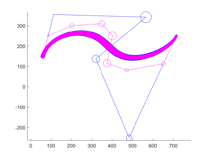
Example 4. (Also Example 2 in [17]) Given a 8 degree disk rational Bézier $(\textbf{p})(t)$ with control disks $(6,14.9)_{1}$ , $(8.6,25)_{0.4}$ , $(20.3,30)_{1}$ , $(35,31)_{1.5}$ , $(40.2,25)_{2}$ , $(37.5,11.5)_{1.8}$ , $(47.2,8.1)_{0.8}$ , $(65.1,11.2)_{1}$ , $(71.5,25)_{0.5}$ and associated weights 1.88, 1.68, 1.63, 1.73, 1.79, 2.18, 1.24, 1.08, 1.9. The best 3-degree reduction curve satisfying $C^{(1,1)}$ -continuity with the given curve has control disks $(6.0000,14.9000)_{10.4812}$ , $(11.2981,35.4812)_{0.8812}$ , $(56.8670,34.1932)_{26.7312}$ , $(31.7728,13.5463)_{18.6645}$ , $(48.8560,-23.8262)_{13.4812}$ , $(71.5000,25.0000)_{5.4812}$ , and associated weights $0.0023,0.0016,0.0013,0.0020,0.0005,0.0019$ . The resulting curve is illustrated in Figure 4.

Refer to caption — Figure 4: The resulting curve

References

[1] T. W. Sederberg, R. T. Farouki, Approximation by interval bezier curves, IEEE Computer Graphics and Applications 12 (5) (1992) 87–95.
[2] C. Y. Hu, T. Maekawa, E. C. Sherbrooke, N. M. Patrikalakis, Robust interval algorithm for curve intersections, Computer-Aided Design 28(6-7) (1996) 495–506.
[3] C. Y. Hu, N. M. Patrikalakis, X. Z. Ye, Robust interval solid modeling-part i: Representations, Computer-Aided Design 28(10) (1996) 807–817.
[4] C. Y. Hu, N. M. Patrikalakis, X. Z. Ye, Robust interval solid modeling-part ii: Boudary evaluation, Computer-Aided Design 28(10) (1996) 819–830.
[5] F. L. Chen, W. P. Lou, Degree reduction of interval Bézier curves, Computer-Aided Design 32(6) (2000) 571–582.
[6] H. W. Lin, L. G. Liu, G. J. Wang, Boundary evaluation for interval Bézier curve, Computer-Aided Design 34(9) (2002) 637–646.
[7] Q. Lin, R. J, Disk bézier curves, Computer Aided Geometric Design 157(9) (1998) 721–737.
[8] M. Shi, Z. L. Ye, B. S. Kanf, Disk rational Bézier curves (in chinese), Journal Compututer-Aided Design and Computer Graphics 23(6) (2011) 1041–10477.
[9] F. L. Chen, W. Yang, Degree reduction of disk Bézier curves, Computer Aided Geometric Design 21(3) (2004) 263–280.
[10] R. Abedallah, H. Yusuf, Multi-degree reduction of disk Bézier curves with $G^{0}$ - and $G^{1}$ -continuity, Journal of Inequalities and Applications 1 (2015) 307.
[11] G. Farin, Algorithms for rational Bézier curves, Computer-Aided Design 15(2) (1983) 73–77.
[12] T. W. Sederberg, G. Z. Chang, Best linear common divisors for approximate degree reduction, Computer-Aided Design 25(3) (1993) 163–168.
[13] F. Chen, Constrained best linear common divisor and degree reduction for rational curves, Numerical Mathematics-A Journal of Chinese Universities (suppl.) (1994) 14–21.
[14] J. Sun, F. Chen, Y. Qu, Approximate common divisors of polynomials and degree reduction for rational curves, Applied Mathematics 13 (4) (1998) p.437–444.
[15] L. Qin, L. T. Guan, Approximate degree reduction of rational curves and surfaces, Journal Image and Graphics 11(8) (2006) 1062–1067.
[16] H. J. Cai, G. J. Wang, Constrained approximation of rational Bézier curves based on a matrix expression of its end points continuity condition, Computer-Aided Design 42 (2010) 495–504.
[17] M. Shi, Degree reduction of disk rational Bézier curves using multi-objective optimization techniques, IAENG International Journal of Applied Mathematics 45(4) (2015) 18.
[18] Y. Collette, P. Siarry, Multiobjective optimization: principles and case studies, Springer Science & Business Media, 2013.