A computer-assisted proof of Barnette-Goodey conjecture: Not only fullerene graphs are Hamiltonian.

A Barnette graph is a 3-connected planar cubic graph with faces of size at most 6, having no triangles and no two adjacent quadrangles.

We reduce Theorem 1 to the case of Barnette graphs:

Proof. Suppose Theorem 2 true. Let $G$ be a smallest counterexample to Theorem 1. We know that $G$ has at least 318 vertices, since Theorem 1 has already been verified for all cubic planar graphs with faces of size at most 6 on at most 316 vertices [2]. (The number of vertices of a cubic graph is always even.)

Assume $f=v_{1}v_{2}v_{3}$ is a triangle in $G$. If one of the faces adjacent to $f$ is a triangle, then, by 3-connectivity, $G$ is (isomorphic to) $K_{4}$, a Hamiltonian graph. Therefore, all the three faces adjacent to $f$ are of size at least $4$. Let $G_{1}$ be a graph obtained from $G$ by replacing $v_{1}v_{2}v_{3}$ by a single vertex $v$. It is easy to see that $G_{1}$ is a 3-connected cubic planar graph with faces of size at most 6, moreover, every Hamiltonian cycle of $G_{1}$ can be extended to a Hamiltonian cycle of $G$, see Figure 2 for illustration.

From this point on we may assume that $G$ contains no triangles. Let $f_{1}$ and $f_{2}$ be two adjacent faces of size 4 in $G$. Let $v_{1}$ and $v_{2}$ be the vertices they share; let $f_{1}=v_{1}v_{2}u_{3}u_{4}$, let $f_{2}=v_{1}v_{2}w_{3}w_{4}$. We denote by $f_{3}$ (resp. $f_{4}$) the face incident to $u_{3}$ and $w_{3}$ ($u_{4}$ and $w_{4}$, respectively). If both $f_{3}$ and $f_{4}$ are quadrangles, then, by 3-connectivity, $G$ is the graph of a cube, which is Hamiltonian. Suppose $d(f_{4})\geq 5$ and $d(f_{3})=4$. Let $G_{2}$ be a graph obtained from $G$ by collapsing the faces $f_{1}$, $f_{2}$, $f_{3}$ to a single vertex. Again, $G_{2}$ is a 3-connected cubic planar graph with faces of size at most 6, moreover, every Hamiltonian cycle of $G_{2}$ can be extended to a Hamiltonian cycle of $G$, see Figure 2.

Finally, suppose that both $f_{3}$ and $f_{4}$ are of size at most 5. We remove the vertices $v_{1}$ and $v_{2}$, identify $u_{3}$ with $w_{3}$ and $u_{4}$ with $w_{4}$; in this way we obtain a graph $G_{3}$. It can be verified that $G_{3}$ is a 3-connected cubic planar graph with all the faces of size at most 6, unless $G$ is the 12-vertex graph obtained from the cube by replacing two adjacent vertices by triangles, which is impossible since $G$ has no triangles. Again, every Hamiltonian cycle of $G_{3}$ can be extended to a Hamiltonian cycle of $G$, as seen on Figure 3. $\square$

Let $G$ be a graph. For a set of vertices $X$, we denote $G[X]$ the subgraph of $G$ induced by $X$. For a set of vertices $X$, $\emptyset\neq X\neq V(G)$, the set of edges of $G$ having exactly one end-vertex in $X$ form a cut-set of $G$. An edge-cut $(X,Y)$, where $Y=V(G)\setminus X$, is cyclic if both $G[X]$ and $G[Y]$ contain a cycle. Finally, a graph is cyclically $k$-edge-connected if it has no cyclic edge-cuts of size smaller than $k$.

Proof. Suppose that $G$ contains a cyclic $3$-edge-cut $(X,Y)$. Choose $X$ inclusion-wise minimal. It is easy to see that the cut-edges are pairwise non-adjacent. Let $x_{1}$, $x_{2}$, $x_{3}$ be the vertices of $X$ incident to the cut-edges. We prove that they are pairwise non-adjacent: Suppose that two of them, say $x_{1}$ and $x_{2}$, are adjacent. Then, by minimality of $X$, $X^{\prime}=X\setminus\{x_{1},x_{2}\}$ is acyclic with $(X^{\prime},V(G)\setminus X^{\prime})$ being a 3-edge-cut, and hence, $|X^{\prime}|=1$, $X^{\prime}=\{x_{3}\}$, so thus $G[X]$ is a triangle, which is impossible in a Barnette graph.

Let $y_{i}$ be the other endvertex of the cut-edge incident to $x_{i}$, $i=1,2,3$. We prove that these three vertices are also pairwise non-adjacent: Since $G$ has no triangles, $G[\{y_{1},y_{2},y_{3}\}]$ has at most two edges. If it had exactly two edges, then $G$ would contain a 2-edge-cut, which is impossible. Suppose now that $y_{1}$ and $y_{2}$ are adjacent, but $y_{3}$ is not adjacent to any of them. Each of the two faces incident to the edge $x_{3}y_{3}$ has at least three incident vertices in both $X$ and $Y$, therefore, it is a hexagon, and there are exactly three incident vertices in both $X$ and $Y$. Let $z_{i}$ be the common neighbor of $y_{3}$ and $y_{i}$, $i=1,2$. Then $z_{1}$ and $z_{2}$ are adjacent, otherwise there would be a 2-edge-cut in $G$. But then $y_{3}z_{1}w_{2}$ is a triangle in $G$, a contradiction.

As $y_{1}$, $y_{2}$, $y_{3}$ are pairwise non-adjacent, for each face incident to any cut-edge, there are at least three incident vertices in both $X$ and $Y$, therefore, each such face is a hexagon having three incident vertices in both $X$ and $Y$. Let $x_{ij}$ be the common neighbor of $x_{i}$ and $x_{j}$, $1\leq i<j\leq 3$. By minimality of $X$, $X^{\prime}=X\setminus\{x_{1},x_{2},x_{3},x_{12},x_{13},x_{23}\}$ is a single vertex, and so $G[X]$ is the union of three 4-faces pairwise adjacent to each other, which is impossible in a Barnette graph. $\square$

Let $f_{1}$ and $f_{2}$ be two faces of an infinite hexagonal grid $H$. Then there is a (unique) translation $\phi$ of $H$ that maps $f_{1}$ to $f_{2}$. The vector $\vec{u}$ defining $\phi$ can be expressed as an integer combination of two unit vectors – those that define translations mapping a hexagon to an adjacent one. Out of the six possible unit vectors, we choose a pair $\vec{u}_{1},\vec{u}_{2}$ making a $60^{\circ}$ angle such that $f_{2}$ is inside this angle starting from $f_{1}$. Then the coordinates $(c_{1},c_{2})$ of $\vec{u}=c_{1}\vec{u}_{1}+c_{2}\vec{u}_{2}$ are non-negative integers, called the Coxeter coordinates of $\phi$ [3].

We may always assume that $c_{1}\geq c_{2}$. The pair $(c_{1},c_{2})$ determines the mutual position of a pair of hexagons in a hexagonal grid, it is also called a Goldberg vector. Observe that, for example, $(1,0)$ corresponds to a pair of adjacent faces, $(1,1)$ corresponds to a pair of non-adjacent faces with an edge connecting them (and thus having two distinct common neighboring faces), whereas $(2,0)$ corresponds to a pair of non-adjacent faces with two paths of length 2 connecting them (and thus sharing a single common neighboring face), etc.

The Coxeter coordinates are used to define nanotubical graphs in the following way:

Let $(c_{1},c_{2})$ be a pair of integers with $c_{1}\geq c_{2}$. Fix a pair of unit vectors $\vec{u}_{1}$ and $\vec{u}_{2}$ making a $60^{\circ}$ angle. A graph obtained from an infinite hexagonal grid by identifying objects (vertices, edges, and faces) whose mutual position is (an integer multiple of) the vector $c_{1}\vec{u}_{1}+c_{2}\vec{u}_{2}$ is the infinite nanotube of type $(c_{1},c_{2})$.

If $c_{1}+c_{2}\leq 2$ then the infinite nanotube is not 3-connected. Since nanotubes with $c_{1}+c_{2}=3$ contain cyclic 3-edge-cuts and Barnette graphs are cyclically 4-edge-connected, we will only be interested in nanotubes with $c_{1}+c_{2}\geq 4$.

Let $N$ be an infinite nanotube of type $(c_{1},c_{2})$. Let $f_{1}$ and $f_{2}$ be two hexagons of the hexagonal grid $H$ at mutual position $(c_{1},c_{2})$ corresponding to the same hexagon $f$ of $N$. Let $P$ be a dual path of length $c_{1}+c_{2}$ connecting the vertices $f_{1}^{*}$ and $f_{2}^{*}$ in $H^{*}$. Then the edges corresponding to the edges of $P$ form a cyclic edge-cut in $H$ of cardinality $c_{1}+c_{2}$. A cyclic sequence of hexagonal faces of $N$ corresponding to the vertices of $P$ is called a ring in $N$.

A finite 2-connected subgraph of an infinite nanotube is an open-ended nanotube if it contains at least one ring. A Barnette graph is a nanotube if it contains an open-ended nanotube of some type as a subgraph. Observe that the same graph may be considered as a nanotube of more than one type.

Let $G$ be a nanotube. We call a cap any of the two inclusion-wise minimal 2-connected subgraphs of $G$ that can be obtained as a component of a cyclic edge-cut defined by a set of edges intersecting a line perpendicular to the vector defining the corresponding open-ended nanotube. See Figures 4, 5, and 7 for illustration.

We omit the details of the proof, as it is similar to the proof of Lemma 2: It suffices to prove that every (potential) cap of a nanotube of type $(3,1)$ or $(2,2)$ contains a triangle or a pair of adjacent quadrangles.

Proof. We may suppose that $G$ has at least $318$ vertices (at least 161 faces). Since the caps of the tube are of bounded size (at most 5, 10, 6, 11, 5, 10, 10, 14 faces, respectively, each), the tubical part of $G$ contains a large number of disjoint rings.

We provide a construction of a Hamilton cycle in such graphs: First, we find a pair of paths covering the vertices of the tubical part of $G$; then, we verify that for each possible cap it is always possible to connect the two paths in a way that all the vertices of the cap are covered as well.

In a nanotube of type $(p,0)$, $p\geq 4$, for each $p$-edge-cut corresponding to a ring, we construct the two paths tranversing the tube in a way that each path contains one cut-edge incident to the same hexagonal face. Let us call this hexagon a transition face. For two consecutive rings, the transition faces are adjacent and once the transition face is fixed for one ring, we are free to choose any of the two adjacent hexagons in the next one to be the transition face, see Figure 4 for illustration.

To complete the proof for $(4,0)$- and for $(5,0)$-nanotubes, it suffices to verify that for every possible cap, there exists a path covering all the vertices of the cap leaving the cap by two edges adjacent to the same hexagonal face of the first ring of the tube. Since the tubical part of $G$ is sufficiently long, we can choose a transition face in the first and the last ring of hexagons regardless of the relative position of the two caps.

For nanotubes of type $(3,3)$, the construction is described in Figure 5.

For nanotubes of type $(p_{1},p_{2})$ with $p_{1}>p_{2}>0$, we provide a repetitive pattern to cover the tubical part (see Figure 6) and, for every cap and for every position of the cap with respect to the pattern, a path covering the vertices of the cap (see Figure 7 for the first two types of nanotubes; we omit the details for the remaining three types). $\square$

Let $H$ be a plane cubic graph. We denote $H^{\parallel}$ the $6$-regular multigraph obtained from $H$ by replacing each edge by a pair of parallel edges, equipped with the following black-and-white face-coloring: We color the 2-gons between pairs of parallel edges white and we color the faces of $H^{\parallel}$ corresponding to the faces of $H$ black. It is easy to see that this is a proper face-coloring of $H^{\parallel}$.

Let $G$ be a Barnette graph and let $M$ be a perfect matching of $G$. Then $F=E(G)\setminus M$ is a $2$-factor of $G$. A hexagonal face of $G$ incident to three edges of $M$ is called resonant.

There is a canonical face-coloring of $G$ with two colors, say black and white, such that each edge of $F$ is incident to one black and one white face. Let $h$ be a white resonant hexagon. Since it is incident to three edges from $M$, the colors of its neighboring faces are alternating black and white.

We transform $F$ into a $6$-regular plane pseudograph in the following way: First, inside each white resonant hexagon $h$ we introduce a new vertex $v_{h}$. We remove the three edges incident to $h$ from $F$ and we replace them by six new edges, joining $v_{h}$ to all the six vertices incident to $h$. Each of the newly created triangles receives the color of the corresponding face adjacent to $h$. This way we obtain a black-and-white face-colored plane graph with two types of vertices: vertices of degree 2 are the vertices of the underlying Barnette graph, vertices of degree 6 correspond to white resonant hexagons.

Finally, we suppress all vertices of degree 2. This operation may create loops, parallel edges, and even circular edges incident to no vertex, see Figure 8 for illustration. Let $G^{M}$ be the resulting black-and-white face-colored plane 6-regular pseudograph.

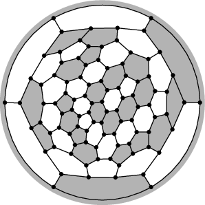
A $2$-factor $F$ is called $\emph{odd}$ if it consists of an even number of (disjoint) cycles; otherwise it is even. The same applies to the corresponding perfect matching.

A $2$-factor $F$ (as well as the corresponding perfect matching $M=E(G)\setminus F$) is called simple if $G^{M}$ has no circular edges and $G^{M}\cong H^{\parallel}$ for some cubic planar graph $H$. If this is the case, $H$ is called the residual graph.

Proof. The number of vertices of a residual graph is always even, since it is a cubic graph. Moreover, the number of cycles in $F$, say $c$, is equal to the number of faces of the residual graph. By Euler’s formula,

so the claim follows immediately.

We will make use of the following classical result:

Observe (by double-counting white-white and black-white edges) that the divisibility condition is a necessary condition for such a partition to exist. That’s why we will only be interested in odd $2$-factors.

Proof. Let $H$ be a cyclically $4$-edge-connected cubic planar graph on $4k+2$ vertices ($k\geq 1$) such that $G^{M}=H^{\parallel}$. Let $F=E(G)\setminus M$. Recall that vertices of $H$ correspond to white resonant hexagons in $G$ with respect to a fixed cannonical face-coloring of $F$. Let $(B,W)$ be a partition of $V(H)$ into an induced (black) stable set $B$ and an induced (white) tree $W$ given by Theorem 3.

We transform the $2$-factor $F$ and the black-and-white face-coloring of $G$ in the following way: For each resonant hexagon $h$ corresponding to a black vertex $b$ of $H$, replace the three edges from $F$ incident to $h$ in $G$ by the other three edges; recolor the hexagon $h$ black. Since $B$ induces a stable set in $H$, this operation can be carried out independently for all black vertices of $H$ at once. For each such vertex, the number of edges from $F$ incident to any vertex of $G$ remains unchanged, therefore, $F$ becomes a $2$-factor of $G$, say $F^{\prime}$.

We claim that it consists of a single cycle. To prove that, it suffices to observe that the graph $(V(G),F^{\prime})$ has a single white face (as $H[W]$ is connected) and a single black face (as $H[W]$ is acyclic). See Figure 9 for illustration. $\square$

It remains to prove that such a situation occurs for at least one perfect matching for any Barnette graph not known to be Hamiltonian yet.

In the rest of the paper, we prove Theorem 4. We describe the general approach in Section 3, and we specify the computer-assisted part in Section 4.

We claim (without proof) that in order to prove Theorem 4 it suffices to consider a simple odd $2$-factor maximizing the number of white resonant hexagons.

We will call a $2^{*}$-factor of a Barnette graph $G$ any spanning subgraph $F$ of $G$ such that each component of $F$ is a connected regular graph of degree 1 or 2 – an isolated edge or a cycle. For a 2^∗-factor $F$ of a Barnette graph $G$, let $F^{(0)}$ be the set of isolated edges of $F$; let $G^{(2)}$ be a plane graph obtained from $G$ by replacing each edge of $F^{(0)}$ by a 2-gon; let $F^{(2)}$ be the set of edges of $G^{(2)}$ corresponding to those from $F$. Then $F^{(2)}$ is a $2$-factor of $G^{(2)}$ in the common (strict) sense.

Given a 2^∗-factor $F$ of a Barnette graph $G$, there are two cannonical black-and-white face-colorings of $G^{(2)}$ (complementary to each other) with the following property: an edge $e$ of $G^{(2)}$ is incident to a white and a black face if and only if $e$ belongs to $F^{(2)}$ (otherwise $e$ is incident to two faces of the same color).

A $2^{*}$-factor $F$ of a Barnette graph $G$ is called quite good if for each of the two canonical black-and-white face-colorings of $G^{(2)}$ induced by $F^{(2)}$ the 2-gons corresponding to the edges of $F^{(0)}$ have all the same color. Given a quite good $2^{*}$-factor of a Barnette graph $G$, we will always assume that a canonical coloring of $G^{(2)}$ such that all the 2-gons of $G^{(2)}$ are black is given along.

A quite good $2^{*}$-factor $F$ of a Barnette graph $G$ is called good if, after having fixed a planar embedding of $G$ such that the outer face is a white one, no cycle of $F$ is inside another.

Observe that given a good $2^{*}$-factor $F$ of $G$, for any planar embedding of $G$ with a white outer face, the set of faces inside a fixed cycle $C$ of $F$ is always the same and these faces correspond to a sub-tree of the dual graph $G^{*}$ (empty if $C$ is a 2-cycle).

Proof. Let $n$ be the number of vertices of $G$, let $f_{k}$ be the number of all faces of size $k$ in $G$, let $x_{k}$ be the number of black faces of size $k$ in $G$. Euler’s formula yields $n=8+f_{5}+2f_{6}$. If a cycle covers $c_{4}\geq 0$ quadrangles, $c_{5}\geq 0$ pentagons, and $c_{6}\geq 0$ hexagons, its length is $2+2c_{4}+3c_{5}+4c_{6}$.

Clearly, each vertex is covered by exactly one cycle, thus we have

since only hexagons can be resonant, and thus $f_{k}=x_{k}+q_{k}$ for $k=4,5$. Therefore,

so $q_{5}$ is even. By dividing by two and rearranging the terms we obtain

the claim immediately follows. $\square$

Let $F$ be a good $2^{*}$-factor in a Barnette graph $G$. Let us consider the structure of the graph $G^{(2)}$. We introduce an auxiliary graph $\Gamma=\Gamma_{G}(F)$, defined in the following way: $V(\Gamma)$ is the set of the white non-resonant faces of $G$ (as of $G^{(2)}$). The edges of $\Gamma$ are defined in the next two paragraphs.

Let $C$ be the facial cycle of a (black) 2-gon $f_{0}$ in $G^{(2)}$. Let $f_{0}$ be incident to vertices $u$ and $v$ and adjacent to two (white) faces $f$ and $f^{\prime}$. Then each of $u$ and $v$ is incident to one more face (which has to be white), say $f_{u}$ and $f_{v}$, respectively. Since $f_{0}$ only shares a vertex with $f_{u}$ and with $f_{v}$, the faces $f$ and $f^{\prime}$ are two consecutive white neighbors of $f_{u}$ ($f_{v}$). Therefore, the faces $f_{u}$ and $f_{v}$ cannot be resonant. We add the edge $f_{u}f_{v}$ to $E(\Gamma)$; we call this type of edge of $\Gamma$ white.

Let $C$ be a cycle of $F$ (and of $F^{(2)}$) which is not a facial cycle of a face of $G^{(2)}$. It means that $C$ is a boundary of a union of at least two faces of $G$. We consider every pair of adjacent faces inside $C$. Let $f$ and $f^{\prime}$ be such a pair of faces. Let $u$ and $v$ be the endvertices of the edge incident to both $f$ and $f^{\prime}$. Then each of $u$ and $v$ is incident to a third face (which has to be white), say $f_{u}$ and $f_{v}$, respectively. The faces $f$ and $f^{\prime}$ are two consecutive black neighbors of $f_{u}$ ($f_{v}$). Therefore, the faces $f_{u}$ and $f_{v}$ cannot be resonant. We add the edge $f_{u}f_{v}$ to $E(\Gamma)$; we call this type of edge of $\Gamma$ black.

Observe that for each edge of $\Gamma$, its endvertices are two faces of $G$ at mutual position $(1,1)$. Each edge of $\Gamma$ covers two vertices of $G$ and these pairs of vertices are pairwise disjoint. Therefore, $\Gamma$ is a planar graph.

Let $f$ be a white pentagon of $G^{(2)}$. It cannot be resonant, so $f$ is a vertex of $\Gamma$. Let $f_{1},\dots,f_{5}$ be the faces adjacent to $f$ (sharing an edge with $f$) in $G^{(2)}$. (Observe that some $f_{i}$ can be a 2-face: if it is the case, then there is another face $f_{i}^{\prime}$ adjacent to $f$ in $G$, and adjacent to $f_{i}$ in $G^{(2)}$.) Since the size of $f$ is odd, the number of pairs $(f_{i},f_{i+1})$ (with $f_{6}=f_{1}$) of the same color (both black or both white) has to be odd. If both $f_{i}$ and $f_{i+1}$ are black, then none of them can be a 2-face, and thus there is a black edge incident to $f$ in $\Gamma$. If both $f_{i}$ and $f_{i+1}$ are white, then again none of them can be a 2-face, and the vertex incident to $f$, $f_{i}$, and $f_{i+1}$ is (in $G^{(2)}$) covered by a 2-cycle adjacent both to $f_{i}$ and $f_{i+1}$, and thus there is a white edge incident to $f$ in $\Gamma$. Altogehter, $f$ is a vertex of odd degree in $\Gamma$.

Similarly, for each non-resonant white hexagon $f$, there is an even number of pairs of consecutive adjacent faces of the same color, hence $f$ is a vertex of non-zero even degree in $\Gamma$.

A white quadrangle $f$ is always considered non-resonant. Its degree in $\Gamma$ is also always even, however, it can be equal to 0 if the neighboring faces are colored alternatively black and white.

As a result of these local observations, the graph $\Gamma$ can always be edge-decomposed into a set of paths with endvertices at the white pentagons of $G$, a set of cycles, and, eventually, a set of isolated vertices (corresponding to white quadrangles). The number of paths in the decomposition is equal to $q_{5}/2$, where $q_{5}$ is the number of white pentagons.

Let $G$ be a Barnette graph and let $p_{1}$ and $p_{2}$ be two small faces of $G$. Suppose that there exists an induced dual path $P^{*}$ connecting $p_{1}$ and $p_{2}$ passing only through hexagons. Then if we consider only faces of $G$ corresponding to $P^{*}$, and if we replace the two small faces by hexagons, we obtain a graph with a cannonical embedding into an infinite hexagonal grid. The Goldberg vector $(c_{1},c_{2})$ joining the first and the last hexagon is uniquely determined. We will use this vector to characterize the mutual position of $p_{1}$ and $p_{2}$ in $G$. Observe that the vector of two small faces may depend on the choice of the path joining them, see Figure 10 for illustration.

Graver [8] used the Coxeter coordinates to describe the structure of fullerene graphs. His technique may be extended to a full description of Barnette graphs as well in the following way: A given Barnette/fullerene graph $G$ is represented by a planar triangulation $T$, whose vertices represent the small faces of $G$, and each edge $uv$ is labelled with a Goldberg vector representing the mutual position of the faces represented by $u$ and $v$. The angle between face-adjacent edges (incident to the same triangle of $T$) is well defined and is determined by the labels of the three edges forming the triangle. For a vertex of $T$ representing a pentagon (a quadrangle) the angles around it sum up to $5/3\pi=300^{\circ}$ ($4/3\pi=240^{\circ}$, respectively).

The existence of a triangulation $T$ is guaranteed by a structural theorem of Alexandrov (see e.g. [4], Theorem 23.3.1, or [15], Theorem 37.1), which states (in a more general setting) that any Barnette graph can be embedded onto the surface of a convex (possibly degenerate) polyhedron so that every face is isometric to a regular polygon with unit edge length; it suffice then to triangulate the faces of this polyhedron. Any spanning tree of $T$ may be used to cut the graph $G$ in order to obtain a graph embeddable into the infinite hexagonal grid, see Figure 10 for illustration.

We say that a Goldberg vector $\vec{u}=(c_{1},c_{2})$ is shorter than $\vec{u}^{\prime}=(c_{1}^{\prime},c_{2}^{\prime})$ if and only if the Euclidean length of a segment determined by $\vec{u}$ is shorter than the Euclidean length of a segment determined by $\vec{u}^{\prime}$ when both embedded into the same hexagonal grid.

Observe that the triangulation representing a Barnette graph is not unique: wherever two adjacent triangles form a convex quadrilateral (once embedded into the hexagonal grid), we may choose the other diagonal of the quadrilateral instead of the existing one as an edge of the triangulation. For example, in the graph depicted in Figure 10 we could have chosen the edge $p_{3}p_{10}$ instead of the edge $p_{2}p_{9}$, etc.

However, for a triangulation $T$ representing a Barnette graph $G$, the operation switching the diagonals of a convex quadrilateral eventually leads to a triangulation minimal with respect to the sum of lengths of its edges. For example, the triangulation depicted in Figure 10 is already minimal.

Proof. Suppose that $T$ has no Hamiltonian path. Then there exists a set $X$ of vertices such that $T\setminus X$ has at least $|X|+2$ connected components. Since $T$ has at most 12 vertices, $|X|\leq 5$.

For each component $C$, the set of vertices in $G\setminus C$ having a neighbor in $C$ contains a cycle in $T$ (as $T$ is a triangulation). Therefore, $G\setminus X$ is a plane graph with $|X|\leq 5$ vertices and $|V(T)\setminus X|\geq 7$ faces.

However, a planar graph on at most 5 vertices can have at most 6 faces. (Adding edges increases the number of faces, and (the) planar triangulation on 5 vertices (the triangular bipyramid) only has 6 faces.) $\square$

Note that the smallest planar graph with desired properties is a bipyramid over a square (which has 6 vertices and 8 faces).

Proof. Suppose that $T$ has no Hamiltonian cycle. Then there exists a set $X$ of vertices such that $T\setminus X$ has at least $|X|+1$ connected components. Since $T$ has at most 12 vertices, $|X|\leq 5$.

For each component $C$, the set of vertices in $G\setminus C$ having a neighbor in $C$ form a cycle in $T$ (as $T$ is a triangulation). Therefore, $G\setminus X$ is a plane graph with $|X|\leq 5$ vertices and $|V(T)\setminus X|\geq 6$ faces.

There is only one such graph: the triangular bipyramid $B$, which has $5$ vertices and $6$ triangular faces. Out of the six components of $T\setminus B$, at least five are singletons, the sixth may eventually be an isolated edge. It means $T$ has five vertices of degree at least 6, six vertices of degree 3, and eventually a vertex of degree 4.

Let $e=uv$ be an edge of $B$. It is incident to two triangles, each incident to a different component of $T\setminus B$. Let $x$ and $y$ be the vertices of $T\setminus B$ such that $uvx$ and $uvy$ are triangles of $T$. If the quadrilateral $uxvy$ is convex, then the triangulation $T^{\prime}$ obtained from $T$ by switching $uv$ to $xy$ has at most five vertices of degree 3, so $T^{\prime}$ has to be Hamiltonian.

It remains to consider the case when for each edge $e$ of $B$, the union of the two incident triangles is a non-convex quadrilateral, meaning that at one of its endvertices, the sum of the angles in the incident triangles is greater than $180^{\circ}$. Since $B$ has five vertices and nine edges, there is at least one vertex of $B$ with two (disjoint) pairs of incident triangles whose union gives a non-convex angle. But then the sum of the angles around this vertex is greater than $360^{\circ}$, a contradiction. $\square$

In Figure 11, an example of a Barnette graph on 322 vertices is depicted, along with the corresponding triangulation and a shortest Hamilton cycle in it.

Let $G$ be a Barnette graph, let $T$ be a Hamiltonian triangulation capturing the mutual position of the small faces of $G$, whose existence is given by Lemma 9. Let $C_{T}$ be a Hamiltonian cycle in $T$ such that the sum of the lengths of the corresponing Goldberg vectors is minimal. Then there exists a cycle $C^{*}$ in $G^{*}$ including all the small vertices of $G^{*}$ in the same order as the corresponding vertices or $C_{T}$.

A cycle in $G^{*}$ corresponds to an edge-cut in $G$. We cut the graph $G$ along $C^{*}$. We obtain two graphs, say $G_{1}$ and $G_{2}$, containing only hexagons as internal faces, and with semi-edges and partial faces on the boundary.

Both $G_{1}$ and $G_{2}$ are subgraphs of the hexagonal grid, hence there is a canonical face coloring using three colors for each of them. We will use colors 1, 2, 3 for one and colors $A$, $B$, $C$ for the other. We color the partial faces in both graphs too.

We choose one color in each graph, say 1 and $A$ (there are 9 color combinations in total), and recolor black all the faces of $G_{1}$ and $G_{2}$ colored 1 or $A$; we color white the other faces. (Later we will inspect all the nine colorings.) This gives a black-and-white face-coloring $\phi_{i}$ inducing a $2$-factor $F_{i}$ in $G_{i}$, $i=1,2$.

Observe that for any choice of a color in $G_{i}$ ($i=1,2$), the edges incident to one face of the other two colors each form a matching $M_{i}$ such that $G_{i}^{M_{i}}=H_{i}^{\parallel}$, where $H_{i}$ is the graph whose vertices are the centers of the faces of the other two colors.

We merge the two black-and-white face-colorings $\phi_{1}$ and $\phi_{2}$ of $G_{1}$ and $G_{2}$, respectively, into an intermediate black-and-white (multi-)face-coloring $\phi^{(i)}$ of $G$ in the natural way: A face not corresponding to a vertex of $C^{*}$ inherits a color from either $G_{1}$ or $G_{2}$; A face which is cut by the cycle $C^{*}$ is divided into two partial faces, one inheriting a color from $G_{1}$ and the other from $G_{2}$, see Figure 12 for illustration.

Let $P^{*}_{i}$ be an active segment, let $\varphi_{i}(1)=B$. Suppose without loss of generality that $\varphi_{i}^{-1}(A)=2$. Then all the faces of $P_{i}$ colored $A$ (and 2) or $1$ (and $B$) are partially black and partially white; both parts of each face of $P_{i}^{*}$ colored $C$ and 3 are white.

We approximate the dual path $P^{*}_{i}$ by a sequence $Q_{i}$ of faces colored $C$ and/or 3, each consecutive pair of faces in a mutual position $(1,1)$.

Let $f$ be a white ($C$- and $3$-colored) hexagonal face of $Q_{i}$. Then among its neighbors, there is a cyclic sub-sequence of $A$- and $B$-faces colored alternatively black and white, and another cyclic sub-sequence of $1$- and $2$-faces colored alternatively black and white, with the coloring being the opposite of the first one. Therefore, there are exactly two pairs (not necessarily disjoint) of adjacent faces of the same color: each pair is either a black $A$-face adjacent to a black $1$-face, or a white $B$-face adjacent to a white $2$-face. Therefore, $f$ is a white non-resonant hexagon, corresponding to a vertex of degree 2 in the future auxiliary graph $\Gamma$ being constructed – we will call it a $\Gamma$-face.

Let $f$ and $f^{\prime}$ be two consecutive $\Gamma$-faces. If the two faces adjacent both to $f$ and $f^{\prime}$ are black, then the two cycles of the $2$-factors in $G_{1}$ and $G_{2}$ are merged. If the two faces adjacent both to $f$ and $f^{\prime}$ are white, then a new 2-cycle of the $2^{*}$-factor is created. In the first case, the $\Gamma$-edge $ff^{\prime}$ is black, in the second case it is a white one.

Two consecutive $\Gamma$-edges of $Q_{i}$ of the same color always form a $180^{\circ}$ angle, otherwise it could be possible to simplify $Q_{i}$ by removing a face from $Q_{i}$. Similarly, two consecutive edges of $Q_{i}$ of different colors always form an angle of $\pm 120^{\circ}$.

The resulting structure of $\phi^{(i)}$ along $P^{*}_{i}$ is the following: All vertices are covered by cycles of length 6 (single faces), 10 (two adjacent black hexagons, both incident to a black $\Gamma$-edge), or 2 (white $\Gamma$-edges). A $\Gamma$-path $Q_{i}$ separates the two subgraphs of regular coloring. See Figure 14 for illustration.

The first (the last) $\Gamma$-face of $Q_{i}$ is the pentagon $p_{i}$ ($p_{i+1}$) if and only if the segment $P^{*}_{i-1}$ ($P^{*}_{i+1}$) is inactive; otherwise the first (the last) $\Gamma$-face of $Q_{i}$ is a hexagon adjacent to $p_{i}$ ($p_{i+1}$) and it is the last (the first) $\Gamma$-face of $Q_{i-1}$ ($Q_{i+1}$, respectively).

White non-resonant hexagons where two consecutive sequences $Q_{i-1}$ and $Q_{i}$ meet are the only occasion where two $\Gamma$-edges of the same color might form a $60^{\circ}$ angle – if only they are both incident to the same pentagon.

Let us explicit the structure of $H^{(i)}=H_{1}\cup H_{2}$ and of $\Gamma$ now: Vertices of $H^{(i)}$ are all the vertices corresponding to faces of $G$ white in $G_{1}$ or in $G_{2}$; each vertex of $\Gamma$ where two black edges meet corresponds to a 2-vertex in $H^{(i)}$ (the corresponding face of $G$ is a non-resonant white hexagon adjacent to four black faces belonging to two different components of the $2^{*}$-factor); each vertex of $\Gamma$ where two white edges meet corresponds to a 4-vertex in $H^{(i)}$ (the corresponding face of $G$ is incident to four different compents of the $2^{*}$-factor, including two 2-cycles); each vertex of $\Gamma$ where a black and a white edge meet at a $120^{\circ}$ angle corresponds to a 3-vertex in $H^{(i)}$ (the corresponding face of $G$ being incident to three different components of the $2^{*}$-factor: a 2-cycle, a 6-cycle and a 10-cycle).

If there are $q_{5}$ white pentagons, then $\Gamma$ is composed of $q_{5}/2$ paths. A white quadrangle is either an isolated vertex of $\Gamma$ (if both incident segments are inactive) or it is an internal vertex of a path (otherwise).

It follows from Lemma 7 that whenever we want to transform an even $2^{*}$-factor into an odd one, it suffices either to increase or decrease the number of black quadrangles by 1, or to increase or decrease the number of black pentagons by 2. In other words, it suffices either to change the number of isolated vertices in $\Gamma$ by 1 or change the number of $\Gamma$-paths by 1.

It suffices now, as the last phase, to transform a good odd $2^{*}$-factor into a simple (odd) $2$-factor. We do it in the following way:

In a good $2^{*}$-factor, each 2-cycle corresponds to a white $\Gamma$-edge $ff^{\prime}$, incident to two white resonant hexagons $h_{1}$ and $h_{2}$ (one in each of $G_{1}$ and $G_{2}$). We can choose either $h_{1}$ or $h_{2}$, say $h_{i}$, and recolor it black: By doing this, the 2-cycle is merged with two other cycles in $G_{i}$; the other face $f_{0}$ incident to both cycles being merged loses its resonantness, it becomes another $\Gamma$-face inserted to the $\Gamma$-path between $f$ and $f^{\prime}$, joint now to $f$ and $f^{\prime}$ by two black $\Gamma$-edges forming a $60^{\circ}$ angle and replacing the original white $\Gamma$-edge. In $H^{(i)}$, a vertex of degree 3 is removed, and thus the degree of three other vertices is decreased by 1: one of them corresponds to $f_{0}$, the other two correspond to $f$ and $f^{\prime}$.

Observe that this operation decreases the number of components of the factor by 2, therefore, starting with an odd factor we can only obtain odd factors.

We make a decision for all white $\Gamma$-edges sequentially according to their order along $Q_{i}$, according to the following rules: If a white $\Gamma$-edge $e_{j}$ forms a $180^{\circ}$ angle with $e_{j-1}$ (which has to have been white in this case) and that we have decided to recolor black a hexagon in $G_{i}$, $i=1,2$, incident to $e_{j-1}$, then we decide to recolor black a hexagon in $G_{3-i}$ incident to $e_{j}$. If a white $\Gamma$-edge $e_{j}$ forms a $120^{\circ}$ angle with a black $e_{j-1}$, we decide to recolor black a hexagon incident to $e_{j}$ in such a way that one of the new black $\Gamma$-edges forms a $180^{\circ}$ angle with $e_{j-1}$.

The resulting structure in $G$ is the following: All the $\Gamma$-paths and $\Gamma$-cycles are formed of black $\Gamma$-edges only. Each vertex of $\Gamma$ of degree 1 or 2 corresponds to a 2-vertex in $H^{(i)}$.

References

- [1] R.E.L. Aldred, S. Bau, D.A. Holton, and B.D. McKay, NonHamiltonian 3-Connected Cubic Planar Graphs, SIAM J. Discrete Math. 13 (1) (2000), 25–32.
- [2] G. Brinkmann, J. Goedgebeur, and B.D. McKay, The Generation of Fullerenes, J. Chem. Inf. Model., 52 (11) (2012) 2910–2918.
- [3] H.S.M. Coxeter, Virus macromolecules and geodesic domes, in A spectrum of mathematics; ed. by J.C. Butcher, Oxford University Press/Auckland University Press: Oxford, U.K./Auckland, New-Zealand (1971) 98–107.
- [4] E. D. Demaine and J. O’Rourke, Geometric folding algorithms. Cambridge University Press, Cambridge, 2007.
- [5] R. Erman, F. Kardoš, and J. Miškuf, Long cycles in fullerene graphs, J. Math. Chem. 46 (4) (2009), 1103–1111.
- [6] P.R. Goodey, A class of Hamiltonian polytopes, (special issue dedicated to Paul Turán) J. Graph Theory 1 (1977) 181–185.
- [7] P.R. Goodey, Hamiltonian circuits in polytopes with even sided faces, Israel J. Math. 22 (1975) 52–56.
- [8] J.E. Graver, Catalog of All Fullerenes with Ten or More Symmetries, DIMACS Series in Discrete Mathematics and Theoretical Computer Science 69 (2005) 167–188.
- [9] S. Jendrol’ and P. J. Owens, Longest cycles in generalized Buckminsterfullerene graphs, J. Math. Chem. 18 (1995) 83--90.
- [10] F. Kardoš and R. Škrekovski, Cyclic edge-cuts in fullerene graphs, J. Math. Chem. 44 (2008), 121–132.
- [11] D. Král’, O. Pangrác, J.-S. Sereni, and R. Škrekovski, Long cycles in fullerene graphs, J. Math. Chem. 45 (4) (2009), 1021--1031.
- [12] K. Kutnar and D. Marušič, On cyclic edge-connectivity of fullerenes, Discrete Appl. Math. 156 (10) (2008), 1661–1669.
- [13] J. Malkevitch, Polytopal graphs, in Selected Topics in Graph Theory (L. W. Beineke and R. J. Wilson eds.), 3 (1998), 169–188.
- [14] D. Marušič, Hamilton Cycles and Paths in Fullerenes, J. Chem. Inf. Model., 47 (3) (2007), 732–736.
- [15] I. Pak, Lectures on discrete and polyhedral geometry. Online book. http://www.math.ucla.edu/~pak/book.htm.
- [16] C. Payan and M. Sakarovitch, Ensembles cycliquement et graphes cubiques, Cahiers du Centre D’etudes de Recherche Operationelle 17 (1975), 319–343.
- [17] J. Zaks, Non-Hamiltonian simple 3-polytopes having just two types of faces, Discrete Math. 29 (1980) 87–101.