The AMBRE Project: Parameterisation of FGK-type stars from the ESO:HARPS archived spectra
Abstract
Context. The AMBRE project is a collaboration between the European Southern Observatory (ESO) and the Observatoire de la Côte d’Azur (OCA). It has been established to determine the stellar atmospheric parameters of the archived spectra of four ESO spectrographs.
Aims. The analysis of the ESO:HARPS archived spectra for the determination of their atmospheric parameters (effective temperature, surface gravity, global metallicities and abundance of -elements over iron) is presented. The sample being analysed (AMBRE:HARPS) covers the period from 2003 to 2010 and is comprised of 126 688 scientific spectra corresponding to 17 218 different stars.
Methods. For the analysis of the AMBRE:HARPS spectral sample, the automated pipeline developed for the analysis of the AMBRE:FEROS archived spectra has been adapted to the characteristics of the HARPS spectra. Within the pipeline, the stellar parameters are determined by the MATISSE algorithm, which has been developed at OCA for the analysis of large samples of stellar spectra in the framework of galactic archaeology. In the present application, MATISSE uses the AMBRE grid of synthetic spectra, which covers FGKM-type stars for a range of gravities and metallicities.
Results. We first determined the radial velocity and its associated error for the 15% of the AMBRE:HARPS spectra, for which this velocity had not been derived by the ESO:HARPS reduction pipeline. The stellar atmospheric parameters and the associated chemical index [/Fe] with their associated errors have then been estimated for all the spectra of the AMBRE:HARPS archived sample. Based on key quality criteria, we accepted and delivered the parameterisation of 90 174 (71% of the total sample) spectra to ESO. These spectra correspond to 10 706 stars; each are observed between one and several hundred times. This automatic parameterisation of the AMBRE:HARPS spectra shows that the large majority of these stars are cool main-sequence dwarfs with metallicities greater than -0.5 dex (as expected, given that HARPS has been extensively used for planet searches around GK-stars).
Key Words.
astronomical database: miscellaneous – stars:fundamental parameters – stars:abundances – techniques:spectroscopic – methods: data analysis1 Introduction
In the last decade, astronomy has entered an era of very large data surveys with the scientific goal to expand our understanding of the formation and evolution of the Universe. In particular, several spectroscopic surveys (for a summary see Recio-Blanco (2012)) are dedicated to the study of the Milky Way to comprehend its kinematic and chemical history in detail. The ESA Gaia mission is the pinnacle of all of these spectroscopic surveys during which its Radial Velocity Spectrometer (RVS) will observe tens of millions of stars, for which the radial velocity, atmospheric parameters, and chemical abundances will be determined.
The analysis of such a large quantity of data using ’by-hand’ methods is not feasible on a short time scale. This has pushed the astronomical community to develop complex algorithms able to automatically determine the stellar parameters for large spectral datasets efficiently and reliably. MATISSE (MATrix Inversion for Spectral SynthEsis) is one such algorithm(Recio-Blanco et al. 2006) that has been developed at the Observatoire de la Côte d’Azur (OCA) and is part of the automated pipeline that will analyse and parameterise the spectra from Gaia-RVS.
The AMBRE Project (de Laverny et al. 2013, see), a collaboration between ESO and OCA, will, in the end have converted the archived spectra provided by ESO into a comprehensive spectral library of homogeneously determined stellar parameters: effective temperature (), surface gravity (), metallicity ([M/H]), and the abundance of -elements versus iron ([/Fe). These quantities will be made publicly available to the international scientific community, as advanced data products via the ESO archive. The AMBRE Project has two other main objectives: first, to rigorously test MATISSE on large spectral datasets over a range of wavelengths and resolutions that include those of the Gaia-RVS and, second, to produce a chemo-kinematical map of the Galaxy using the combined ESO archive samples to unravel galactic formation and evolution.
The first part of the AMBRE project consisted of the analysis of the FEROS archived spectra. This has been presented in Worley et al. (2012), and the parameters are now publicly available. The present paper reports the work carried out on the HARPS archived spectra provided by ESO. In Sec. 2, we describe the dataset and its properties, with the adaptation of the AMBRE:FEROS analysis pipeline to the AMBRE:HARPS sample and the derivation of the radial velocities. Section 3 we exaplain how we used a sample of stars with repeated observations to determine the internal error. Section 4 describes the external errors estimates by the comparison of key samples with literature parameter values. Finally, Sec. 5 presents the parameterisation of the accepted AMBRE:HARPS spectra with their delivery to the ESO archive, and we conclude in Sec. 6 with a short summary.
2 The AMBRE analysis of the HARPS spectra
The High Accuracy Radial velocity Planet Searcher (Mayor et al. 2003, HARPS) is a fiber-fed, cross-dispersed echelle spectrograph that was built by a consortium of four institutes: the Observatoire de Genève, the Observatoire de Haute Provence, the Universität Bern, and the Service d’Aéronomie of CNRS in collaboration with ESO. It was installed and commissioned on the ESO 3.6m Telescope at La Silla, Chile, in 200311 1 http://www.eso.org/sci/facilities/lasilla/instruments/harps/index.html. The HARPS high resolution () spectra and the long term instrument stability ensure a radial velocity accuracy of about 1 m s-1 (Lo Curto 2011), making HARPS the prime facility for exoplanet hunting.
The AMBRE analysis of the HARPS spectra comprises of the spectra observed from October 2003 to October 2010. They have been homogeneously reduced by ESO with the HARPS pipeline and made publicly available through the ESO archives. This sample was delivered to OCA from the ESO archive department and it includes calibration and science spectra. The ESO:HARPS pipeline produces different types of science spectra: the extracted 2-Dimensional spectra, where each line contains the extracted flux from one spectral order; the extracted 1-Dimensional spectra, which contains the re-binned and merged spectral orders; and the radial velocity cross correlation function (CCF), which is computed between each order and a template mask. For the AMBRE analysis, we used the 126 688 extracted 1-Dimensional science spectra. About 85% of these spectra have a corresponding CCF spectrum and, thus a radial velocity () estimate. For the remaining 15%, we calculated the using the AMBRE automatic program (see Worley et al. 2012, Sec. 4.2 and Sec. 2.1 of the present paper).
This AMBRE:HARPS sample of 126 688 spectra is composed of several thousands of distinct stars with some of them being observed a few tens of times. We have found that the object ID available in the file header was not always a reliable indicator; thus, we have determined the total number of distinct stars included in this sample by performing a coordinate matching analysis whereby a maximum distance radius was imposed. Within a radius of , we obtain 17 218 distinct stars. The counts of the number of science spectra and, thus, distinct objects that have been observed by HARPS in the given period are reported in Fig. 1 with the number of spectra with calculated by the ESO:HARPS pipeline.
Figure 2 shows the distribution of the repeated observations, which shows the number of different spectra available for the same star within the AMBRE:HARPS sample. About % of the stars were observed only once, and % of the sample less than 20 times. Within the search radius of 5 , we have found that only 182 targets have been observed more then 110 times with a maximum of 1 211 repeated observations for Procyon AB binary system.
2.1 Radial velocity
To analyse the observed spectra with MATISSE, it is necessary to correct them by the radial velocity of the star. Since the main scientific goal of HARPS is the search for exoplanets by measuring variations in the radial velocity of the host star, the data reduction pipeline (DRS) of HARPS determines the radial velocities with extremely high accuracy (1 m s-1). Radial velocity error estimates are also provided. Given the large number of spectra to be analysed and for the purpose of homogeneity with the ESO archives, we chose to adopt the radial velocity and the associated error provided in the header of the delivered reduced spectra when available.
However, as previously mentioned, among the sample of spectra delivered to OCA, approximately do not have a HARPS:DRS radial velocity. Almost all of this subsample of spectra have a radial velocity set to a default value from the DRS, while a tiny fraction () have calculated values that are larger than 500 km s-1 in modulus. This indicates that the DRS radial velocity routine had most likely not converged. We therefore calculated the for this subsample of spectra using the AMBRE pipeline (see Worley et al. 2012, Sec. 4.2). Briefly, the radial velocity routine performs a cross-correlation between each spectrum and a set of 56 synthetic masks specifically computed for the AMBRE:HARPS sample. For each spectrum, the output is therefore a set of 56 radial velocity determinations with associated errors; the radial velocity with the lowest error has been adopted. We point out that a final check on the validity of the adopted has been performed once the analysed spectra have been parametrized. We indeed always found that the atmospheric parameters estimated for a HARPS spectrum and those of the adopted mask agree with each other.
The AMBRE procedure also gives an estimate of the uncertainty associated with the derived radial velocity. To check the consistency of these results with the HARPS , we also determined the radial velocity for a sample of spectra having a computed by HARPS:DRS. For that purpose, we considered a sample of 17 000 HARPS spectra, which were observed in 2004.
This comparison between the HARPS:DRS and the derived by AMBRE is shown in Fig. 3. The distribution of the residuals between the two estimates in the bottom panel of Fig. 3, shows a Gaussian distribution centered close to zero ( km s-1). Additionally, 89% of the spectra have an absolute value of the residual, which is smaller than 1 km s-1, whereas 96% of them have a difference smaller than 2 km s-1. This test confirms the high enough consistency between the HARPS and the AMBRE , such that the use of the AMBRE for those spectra without a HARPS stills provide a homogeneous parameterisation analysis across the entire sample. Moreover, with reference to (Worley et al. 2012, Fig. 11), we note that an error of 2 km s-1 on the radial velocity has very little effect on the determination of the atmospheric parameters.
In summary, we therefore adopted the radial velocity and associated error provided by HARPS:DRS for the AMBRE analysis whenever possible. When these quantities were not available, we calculated them using the AMBRE procedure that has been shown to be consistent with the HARPS:DRS results.

2.2 The AMBRE:HARPS parameterisation pipeline
For the analysis of the HARPS spectra, we started from the pipeline that was developed for the AMBRE:FEROS analysis, which is described in detail in Worley et al. (2012). Due to the inherent differences between the two instruments in configuration (principally resolution and spectral range) and in the ESO reduction pipeline products (the radial velocity is provided for each HARPS spectra, for instance), the AMBRE:FEROS pipeline was adapted to obtain an optimal analysis for the HARPS spectra. These modifications are highlighted in the following subsections.
2.2.1 Adaptation of the HARPS spectra for the AMBRE analysis
The parameterisation of the stellar spectra in AMBRE is performed by a kind of comparison of the observed spectra with a library of synthetic spectra using the MATISSE algorithm (Recio-Blanco et al. 2006). We remind that MATISSE is a local multi-linear regression method. It acts as a projection method in the sense that the input observed spectra are projected onto a set of vectors derived during a learning phase of MATISSE. These vectors are a linear combination of reference spectra (i.e. the synthetic spectra described below) and could be roughly viewed as the derivatives of these spectra with respect to the different stellar parameters. We point out that we adopted exactly the same version of MATISSE for the analysis of the FEROS and HARPS spectra (see comment in Sect. 5.1).
Moreover, the same grid of synthetic spectra, the AMBRE grid, has also been adopted. Shortly, this grid of 17 000 high-resolution synthetic spectra has been computed from MARCS model atmospheres (Gustafsson et al. 2008), taking into account the most complete atomic and molecular linelists. The spectra cover the whole optical domain for cool to very cool stars of any luminosity (from dwarfs to supergiants) with metallicities varying from 10-5 to 10 times the Solar value. Large variations in the chemical composition of the -elements with respect to iron have also been considered. As in the MARCS models, a constant microturbulent velocity has been adopted for dwarfs (1 km/s) and giants (2 km/s). More details on the properties of the AMBRE grid and how it has been computed can be found in de Laverny et al. (2012).
The wavelength coverage of the AMBRE synthetic spectra grid goes from 300 nm to 1 200 nm, which is the whole optical wavelength domain. We, thus, were able to select only those wavelengths corresponding to the HARPS wavelength domain that were useful for the analysis. HARPS disperses light on 68 orders covering the spectral range between 378 nm and 691 nm with a gap from 530 nm to 533 nm due to the two CCDs that form the detector system of the instrument. Since we analysed the extracted 1-Dimensional spectra, we first discarded the blue and red edges of the CCDs where the signal-to-noise (S/N) can be significantly lower with respect to the remainder of the spectrum.
Then, from the two wavelength domains defined by the two CCDs, we rejected sections that contained sky absorption and telluric features. In addition, we rejected the very broad Ca II H & K lines, since they can be poorly synthesised for some parameter combinations and they are difficult to normalise automatically. The accepted wavelength regions for the AMBRE:HARPS analysis are listed in Table 1.
| Region | Min | Max |
|---|---|---|
| (nm) | (nm) | |
| 1 | 400.0 | 500.0 |
| 2 | 513.0 | 530.0 |
| 3 | 552.0 | 566.0 |
| 4 | 575.0 | 580.0 |
| 5 | 600.0 | 627.0 |
| 6 | 635.0 | 645.0 |
| 7 | 661.0 | 685.0 |
A further refined selection of the wavelength ranges was then performed by comparing the observed normalised spectra of the Sun and Arcturus line by line (the two stars are representatives of standard dwarf and giant stars and taken from (Wallace et al. 1998; Hinkle et al. 2000)) with the corresponding synthetic spectra in the AMBRE grid. Lines at matching rest wavelengths were rejected when the percentage difference between their two fluxes was larger then a fixed threshold. After testing, we selected a threshold of 0.05% for the Sun and 0.15% for Arcturus. Both thresholds had to be met for the spectral line to be included. These thresholds removed obvious mismatches between the observed and synthetic spectra. A higher threshold was set for Arcturus since the underlying physics of giants is less understood than it is for the Sun and hence the spectra of giants are not as well synthesised. This threshold is also allowed for greater inaccuracies in normalisation between the Arcturus and its corresponding synthetic spectrum.
This procedure allowed us to define the final list of selected wavelengths for the AMBRE:HARPS parameterisation. It consists of intervals sampling the previously selected HARPS domains reported in Table 1 and spanning a total range of about 147 nm. Using this final list of wavelength intervals, we extracted the corresponding ranges from the grid of synthetic spectra resulting in the AMBRE:HARPS synthetic spectra grid.
As the resolution and pixel sampling of HARPS are very high, the computing time required to analyse the original spectra is also correspondingly high. As for the AMBRE:FEROS analysis, the resolution and pixel sampling can be lowered to optimise computing time but without sacrifying the key spectral informations with the goal being to keep an as good as possible accuracy on the derived stellar parameters. This has been explored in our previous AMBRE:FEROS analysis and we have found that a resolution was sufficient to achieve the required accuracy.
The HARPS spectra have a constant resolution () and hence a varying with (where is the full-width-at-half-maximum (FWHM) of the spectral feature at ). This is contrary to the synthetic spectra, which have been computed without any instrumental nor macroturbolence profiles, and a constant wavelength sampling of 0.001 nm.
By degrading (or convolving) both the synthetic and observed spectra to a lower resolution and mapping the observed FWHM profile onto the synthetic FWHM profile, computation time can be decreased and the comparison between the two sets of spectra is then consistent. The convolution was performed by “smoothing” the spectra with a Gaussian for which the FWHM was greater (and therefore of lower resolution) than that of HARPS.
The synthetic grid was convolved with a Gaussian of FWHM=0.02218 nm to produce a synthetic grid with resolution less than that of HARPS.
For each observed spectrum, the measured variation of as a function of was interpolated to a linear function providing a uniformly increasing FWHM profile for each spectrum (where possible). Similarly, for a subsample of synthetic spectrum in the grid, their FWHM profile was also measured by the same procedure, confirming the constant FWHM profile. The mean value from the combination of all of these synthetic FWHM profiles was found to be FWHM nm, as expected from the grid convolution, confirming that our procedure is valid. This was taken to be the nominal synthetic grid FWHM.
To map the convolution of the observed onto the synthetic for each bin in , the FWHM of the smoothing Gaussian was calculated using FWHMmean and the observed was linearly interpolated FWHM for that bin. This resulted in the convolved observed spectra having a constant FWHM profile of the same resolution as the convolved synthetic grid.
The final wavelength sampling was chosen to fulfill the Shannon criterion resulting in a sampling of 0.0085 nm/pixel. The same sampling was also applied to the synthetic spectra of the AMBRE:HARPS grid from which we generated the learning functions of MATISSE to parameterise the observed spectra. We remind that the broadening caused by the micro-turbulent velocity is dominated by the adopted one for the analysis. In consequence, this parameter is not estimated by the pipeline that relies on the adopted constant micro-turbulent velocity of the synthetic grid. We also do not derive the projected rotational velocity and reject every spectra having a too large line-broadening that could affect our parameter estimates (see our discussion in Worley et al. (2012)).
2.2.2 Spectral processing A, B and C
In Worley et al. (2012, Sec. 4 and Fig. 4), a detailed description of the several steps that are part of the AMBRE pipeline with a graphical representation of the process is reported. We review the three main stages of the AMBRE pipeline here. We refer the reader to the AMBRE:FEROS analysis for more detail.
First, we remind that the HARPS spectra delivered to us by ESO are the products of the standard data reduction pipeline. As a consequence, some degradations could still be present in some spectra as, for instance, some possible contaminations by the wavelength calibration lamp for the low S/N ones (about 7% of the whole AMBRE:HARPS sample has S/N 20). To keep the analysis of the whole sample as homogeneous as possible, we preferred to ignore such effects in the following.
In spectral processing A (SPA), the observed spectra are prepared for radial velocity computation and spectral FWHM measurements, and a first quality check is performed identifying noisy or problematic spectra. Each spectrum is sliced in the wavelength regions defined above and roughly normalised to unity. Previously in Worley et al. (2012), the spectral FWHM was measured during the next stage. However, as this was heavy in computing time, it has been developed as a standalone routine for AMBRE:HARPS and AMBRE:UVES that can be run in parallel to the radial velocity routine on the normalised spectra of SPA. The radial velocity program was used only on the spectra for which the HARPS radial velocity was not available, and the radial velocity testing sample (see Section 2.1). During SPA, we calculated the S/N of the spectra (since it was not reported in the header of the reduced spectra), as done in the AMBRE:FEROS analysis.
Spectral processing B (SPB) is the stage at which the first estimate of the stellar parameters is made using MATISSE. The observed spectra are, thus, normalised and convolved to be consistent with the AMBRE:HARPS synthetic grid. At this stage, there is still no determination of the atmospheric parameters; thus, the spectra are normalized to unity. A key point is also the flagging and rejection of problematic spectra; spectra flagged as “bad normalized”, “noisy” or “missing wavelength” are rejected before the subsequent stage. We point out that, contrary to the SPB of Worley et al. (2012), no iteration were performed for the HARPS spectra in SPB since the SPB estimate of the stellar parameters was always close to the final solution.
Finally, rather than normalisation to unity, the normalisation of each spectrum in Spectral Processing C (SPC), is performed on a synthetic spectrum to better represent the continuum placement of the star. In the first instance, the normalisation is performed on the synthetic spectrum generated at the stellar parameters of the solution found in SPB. The resulting normalised spectrum is then analysed in MATISSE, which provides yet another solution and corresponding synthetic spectrum. Thus, SPC consists in iterating between normalisation and parameterisation, ultimately converging on the final stellar parameters, the final normalised spectrum and the final synthetic spectrum. A quality flag is produced, based on a fit between the observed spectrum and synthetic spectrum at the determined stellar parameters.
2.2.3 Rejection criteria
The final parameters delivered to the ESO archive are a subsample of the entire set of parameters estimated by our pipeline due to quality selection based on several rejection criteria. As in Worley et al. (2012, Sec. 7), the first set of rejection criteria that were applied were based on the radial velocity error (), the FWHM of the CCF, the S/N, and the quality of the fit of the normalised spectra to the synthetic spectra ():
- •
Following the rejection procedure of the AMBRE:FEROS data, all HARPS spectra with km s-1 were rejected as corresponding to large uncertainties in the parameter determination, see Worley et al. (2012, Sec. 3 & 5.2 and Fig. 11). Specifically, for such large errors on the radial velocity, the uncertainties would be greater than K in , dex in , dex in [M/H] and dex in [/Fe]. This step resulted in the rejection of 14 105 spectra (11% of the total sample).
- •
With reference to Worley et al. (2012, Sec. 7.2.3), all spectra with a FWHM of the CCF larger than 20 km s-1 (hot/fast rotating stars) were rejected. Such a threshold value was also chosen on the basis of the results obtained by Gazzano et al. (2010). It excluded another 5 199 spectra from the final results (4% of the total).
- •
We also excluded every spectra having a S/N smaller than 10, since the parameterisation of such spectra are associated with rather large internal errors (see Sec. 3).
- •
Finally, to apply a rejection criterion based on the S/N of the HARPS spectra with the quality of their parameterisation, we first divided the remaining set of spectra into three different temperature domains: hot stars (T K), warm stars (5 000 K 6 500 K) and cool stars (4 000 K 5 000 K). For each of the three temperature domains, the S/N threshold used to reject spectra was determined by fitting a second degree polynomial to the distribution of as a function of the S/N. This corresponds to the sum of the squared differences between the synthetic and observed fluxes performed at every pixel:
(1) We investigated the effect of applying different thresholds in the three temperature domains by looking at the distribution of the rejected spectra in the HR diagram. The optimal selection for cool stars was obtained by retaining all the spectra below 0.5 times the standard deviation above the fit for cool stars. Similarly, we kept the warm star spectra by having a smaller than three times the standard deviation above the fit (see Fig. 4 and Table 3) and finally, every hot star spectra located below the fit in the S/N- space. This last stage resulted in the rejection of 6 340 spectra (5% of the total).

As last rejection criterion, we applied the restrictions imposed by the synthetic grid boundaries, particularly excluding stars cooler then 4 000 K, since the determination of gravity was uncertain in the temperature range between 3 000 K and 4 000 K. The adopted grid limits are as follows:
- •
4 000 K Teff 7 625 K;
- •
1 dex 5 dex;
- •
-3.5 dex [M/H] 1 dex;
- •
-0.4 dex [/Fe] 0.4 dex if [M/H] 0.0 dex;
- •
-0.4 dex [/Fe] 0.8 dex if -1.0 dex [M/H] 0.0 dex;
- •
0.0 dex [/Fe] 0.8 dex if [M/H] -1.0 dex.
After the application of these rejection criteria, stellar parameters for 93 116 spectra were accepted (i.e. 73% of the initial sample). The stellar parameters derived for this AMBRE:HARPS sample of spectra are described in Sec. 5.
3 Internal error analysis
An estimate of some of the contributions to the internal errors associated with the analysis can be provided by injecting a large sample of interpolated (at random stellar parameter values) noised synthetic spectra with different uncertainties in radial velocity (see Worley et al. 2012, Sec. 5) into the pipeline. We point out that we only test the performances of the MATISSE method itself here by checking its ability to retrieve the atmospheric parameters in a very ideal case, since only a Gaussian white noise is assumed, and any possible mismatch between the synthetic and real spectra are assumed to be negligible. Since synthetic spectra that are almost the same spectral resolution and spectral coverage were used for AMBRE:HARPS as for AMBRE:FEROS, the error analysis of AMBRE:FEROS can be considered as valid for the analysis of the AMBRE:HARPS spectra. As shown in Worley et al. (2012):
- •
the behaviour of the 70th percentile of the internal error of each atmospheric parameter as a function of the S/N show that for the internal errors are negligible and, thus, have almost no effect on the determined parameters (see Worley et al. 2012, Fig. 10). Since only the HARPS spectra with have been retained, this argument is valid for the present parameterisation.
- •
The error on radial velocity for the accepted sample has a small effect on the determination of the stellar parameters. We reached this conclusion on the basis of Worley et al. (2012, Fig. 11) and our Fig. 5. In Worley et al. (2012, Fig. 11), the behaviour of the percentile of the variation in each photospheric parameter calculated from the same spectrum as a function of artificial variations in the value of is reported. There, it is shown that the percentile value for each parameter is relatively small for km s-1 (even smaller if is limited to 6 km s-1). Figure 5 shows that almost all the spectra () that passed the rejection criteria described in Sec. 2.2.3 have a km s-1. Putting together this result with what reported above, we conclude that we neglect hereafter the contributions of uncertainties and low-quality spectra to the internal errors, since every spectra with and error in greater than 10 km s-1 has been rejected.
The other possible sources of internal errors (and particularly any possible mismatch among observed spectra, real spectra and the effects of the real noise of the spectra) have been investigated by considering a second independent method. It consisted in estimating the internal error of the AMBRE:HARPS analysis by comparing the parameterisation of the repeated observations of the same star, which are characterized by different S/N and uncertainty on the radial velocity.
For that purpose, the sample of 93 116 parameterised spectra were investigated to identify those stars, which had been observed by HARPS at least 50 times, adopting a coordinate search radius of 5″. Using the web tool SIMBAD, we identified and then excluded from this repeat sample the observations of multiple stellar systems and variable stars, since the stellar parameters of these objects could vary with time.
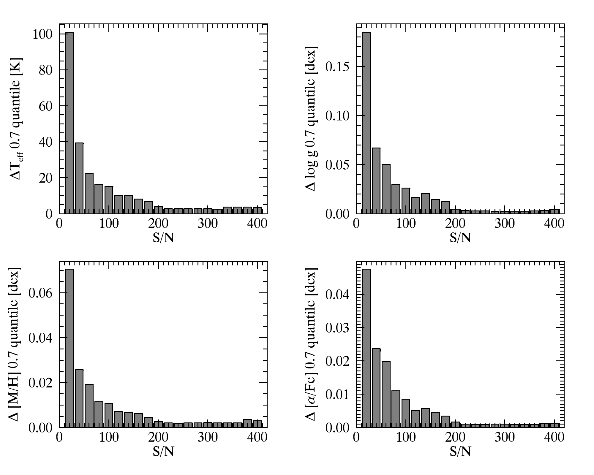
This resulted in a sample of 61 313 spectra that corresponded to 6 094 distinct stars observed 50 times or more as per the radius search. For each set of repeated observations, the mean value of each stellar parameter and the deviations from the mean values for each spectrum was calculated. In this way, we ended up with deviations from mean values as functions of S/N. The sets of repeat spectra were then sorted by their S/N to compute the 0.7 quantile of the parameter deviations for bins of .
The results reported in Fig. 6 show that the deviations in each stellar parameter decrease with increasing S/N, as expected. These trends were used to define the internal errors as follows. For a given spectrum with an associated S/N, the 0.7 quantile-value in the corresponding S/N-bin was adopted as the estimate of the internal error of the AMBRE:HARPS parameterisation.
For spectra with S/N > 160, a lower limit for the internal errors (set by the MATISSE internal error) was adopted as follows:
- •
K;
- •
dex;
- •
dex;
- •
dex.
4 External error analysis
To quantify the external errors associated with the AMBRE:HARPS stellar parameters, they were compared with literature values for key samples within the dataset.
4.1 Benchmark stars
As a first estimate of the quality of this analysis, the results of the AMBRE:HARPS pipeline were investigated for a sample of well-studied reference stars. This sample is the FGK benchmark star sample defined for the Gaia mission and the Gaia ESO Survey (GES), for which the parameters are based on the homogeneous analysis of high quality data. For these benchmarks, we adopted the effective temperatures and surface gravities of Heiter et al. (2014, in prep.) with the metallicities from Jofré, P. et al. (2014). Currently, there are no reference abundances of the -elements available for these stars. We show the comparison between the AMBRE:HARPS and reference values for the stellar parameters of the ten FGK benchmark stars, which have a HARPS spectrum with S/N within the AMBRE:HARPS dataset in the three panels of Fig. 7. The agreement is very good between both set of parameters with low biases and standard deviations, validating the results of the AMBRE:HARPS analysis for cool dwarfs with metallicities higher than dex (i.e. the greater majority of the AMBRE:HARPS sample, see below). We, however, point out that the agreement is slightly less good for the derived surface gravity of HD 22879 and the overall metallicity of the hot star Procyon, whose spectrum exhibits less metallic lines than the bulk of the AMBRE:HARPS sample.


4.2 Porto sample
An independent group previously published a large dataset of stellar atmospheric parameters estimated from HARPS spectra (Porto sample, hereafter) (Sousa et al. 2008; Sousa et al. 2011b; Sousa et al. 2011a; Adibekyan et al. 2012; Tsantaki et al. 2013, see). This sample consists in stars for which stellar parameters have been estimated using a completely different method than that employed here, since the Porto method is based on an equivalent widths analysis of several selected lines.
The results of the Porto analysis provide a unique opportunity to perform a comparison between the parameterisation performed by two independent methods (with different line lists, model atmospheres, spectral analysis techniques, etc.) that analysed the same significantly large quantity of high quality spectra produced by the same instrument. Furthermore, this allows us to conduct a robust estimation of the external errors of the AMBRE:HARPS pipeline. Before describing the comparison between the two samples, we remind here that the AMBRE pipeline derives a mean [M/H] (i.e. taking into account all the metals), while the Porto group derives the [Fe/H] metallicity by considering only iron lines.
A cross match between the coordinates of the Porto sample and AMBRE:HARPS using a radius of 5 ″revealed 713 stars have been analysed by both methods. These 713 stars correspond to 3 991 spectra in the AMBRE:HARPS dataset with S/N ranging from 20 to 221 (see Fig. 8). For the purpose of this comparison, the mean value of the derived AMBRE:HARPS stellar parameters (and the associated standard deviations) were calculated to represent the star when several spectra were available for the same star. The AMBRE:HARPS parameters were then compared to the Porto values in Fig. 9.
The agreement between the Porto and AMBRE:HARPS stellar parameters are also illustrated in Fig. 10 where the distribution of the residuals from the median value for each parameters are shown. The main characteristic of these distributions is that they are not perfectly centered on zero, but rather small biases exist that have been estimated as the mean value of the differences between Porto and AMBRE:HARPS.
Figure 9-top left shows the comparison between the two set of effective temperatures. Despite the difference in the two methods, there is very good agreement between both results, the bias being around K, and the dispersion around 87 K. It can be noted that the updated Porto effective temperatures of Tsantaki et al. (2013) for the cooler stars (below 5 000 K) are based on a new line list specifically built for these cool stars, which considerably improved the agreement in that temperature range. Indeed, their previous effective temperatures were slightly higher, leading to an absolute value of the bias between Porto and AMBRE:HARPS of 86 K (with standard deviation of 128 K) for the effective temperatures between 4 000 and 5 000 K. These bias and standard deviations decreased to an absolute value of 26 K and 117 K, respectively, when adopting the Porto revised values. In Figure 9 we also point out that, the small tail at large negative values is produced by stars hotter than 6 000 K, which are more difficult to parametrize than cooler stars.
The agreement is not as good but still very reasonable for the stellar gravity comparison (see Fig. 9), as it is probably the most difficult stellar atmospheric parameter to derive. The bias in gravity is dex, and the standard deviation is 0.19 dex. In Fig. 9, it can be seen that the possible cause of this bias and standard deviation could be that the Porto stellar gravities seem to span a smaller range of values than those obtained with the AMBRE:HARPS pipeline. Most of their sample data are indeed found between 4.3 and 4.6 dex, while the AMBRE:HARPS are mostly found between 4.2 and 4.7 dex. It can be seen in this figure that the large majority of the discrepant stars have an effective temperature larger than 6 000 K and/or a metallicity smaller than -0.4 dex, i.e. the cases for which spectra exhibit rather few lines to perform the parameterisation.
On the other hand, Fig. 9 reveals that the agreement between the stellar metallicities is very good (the bias is almost null and the dispersion is smaller than 0.1 dex). We note that we derive a slightly lower value than Porto, for stars with a mean metallicity smaller than -0.4 dex, and the small discrepancy seems to increase for lower metallicities. Indeed, when considering only stars, which have [M/H]<-0.4 dex, we calculate a bias and a standard deviation of -0.091 dex and 0.076 dex, respectively. Moreover, we point out that these stars are -enriched (see Fig. 9). In any case, the agreement is much better for more metal-rich stars, which consists of the bulk of the total sample.
Finally, it was also possible to compare the abundance ratios of the -elements with respect to iron. Adibekyan et al. (2012) published the individual abundances of the following -species: Mg , Si , Ca , Ti I, and Ti II. The mean of these five abundances was taken to compare to the AMBRE:HARPS [/Fe] ratios (see Fig. 9-lower right panel). Once again, the agreement is very satisfactory with a quasi-null bias and a standard deviation of only 0.03 dex. It can be, however, noted that, a small departure for this [/Fe] ratio comparison, from the one-to-one line is present for the highest values of [/Fe], or the most metal-poor stars (the Porto sample having slightly smaller [/Fe] ratios when [/Fe] 0.2 dex). To understand this behaviour, we studied the values of the mean abundances produced by our pipeline as a function of the abundances of the individual -species provided by Adibekyan et al. (2012). Figure 11 reveals that the disagreement is probably mostly caused by the behaviour of the Ca and Si abundances that depart more than the other -species.
In summary, it can be concluded that the agreement between the Porto and AMBRE:HARPS stellar parameters are very satisfactory. This comparison sample consists mainly of cool dwarf (solar-type) stars, and the agreement, therefore, validates the AMBRE:HARPS results for more than 90% of the spectra found in the AMBRE:HARPS sample. It has, however, to be noted that a lack of a good comparison sample did not allow us to estimate the systematic differences for non solar-type stars (although some estimates are given in Fig. 9 for hot and metal-poor dwarfs, respectively). Finally, we point out that the Porto sample is also probably affected by trends and systematics and that some of the differences with AMBRE:HARPS could also partly originate in the Porto catalogue.


4.3 External error quantification
From the above comparisons, we can conclude that only small biases are found between the AMBRE:HARPS stellar parameters and those of the Gaia Benchmark and Porto samples. We therefore decide to not perform any bias corrections, contrary to what has been done for the AMBRE:FEROS parameters. In this way, we also avoid needing to correct the stellar parameters of the remainder of AMBRE:HARPS spectra sample that are not found within the reference and Porto samples.
As for the external errors associated with the AMBRE:HARPS parameters, they have been defined using the Porto sample, which is a statistically significant comparison sample. It must be noted that the Porto sample has its own sources of error, and therefore, the adopted external errors are probably overestimated. These external errors are estimated from the 0.7 quantiles reported in Fig. 10 and are
- •
K;
- •
dex;
- •
dex;
- •
dex.
We point out that these external errors are based on dwarf star comparisons only. However, these values were also adopted for the few giants of the AMBRE:HARPS sample since (i) there was a lack of a good reference sample for giants in AMBRE:HARPS and (ii) as shown in Worley et al. (2012), except perhaps for the surface gravity, the external errors can be considered as constant for most of the stellar types.
As the final error associated to each parameter will be the quadratic sum of the internal and external errors, we verified the consistency of this value with the deviations of the AMBRE:HAPRS parameters from the reference. Referring to the Porto sample, we confirmed that the error associated to AMBRE:HARPS parameters is a good approximation to the deviations from the literature at all S/N.
5 The AMBRE:HARPS stellar parameters delivered to ESO
5.1 Final parameters of AMBRE:HARPS analysis
The final accepted stellar parameters of the 93 116 AMBRE:HARPS spectra are shown in Fig. 12 (HR diagram), Fig. 13- 15 (histograms of the distribution of the three main stellar parameters), and Fig. 16 (different combinations of the AMBRE:HARPS stellar parameters).
The main characteristic of Fig. 12 is that the great majority of the spectra are populating the main sequence, confirming that more than 90% of the entire HARPS:AMBRE sample constitutes of cool dwarf stars of G and K spectral types (see also Fig. 13, 14, and Fig. 16). Actually, a large fraction () of the spectra correspond to stars with an effective temperature close to the solar. Furthermore, most of these dwarfs (86%) have a solar metallicity, which larger than -0.5 dex (see Fig. 15). The red giant branch is clearly seen, although it is much less populated. From Fig. 14, it can be seen that about 4% of the total sample is composed of giant stars (defined as dex). We refer to a forthcoming paper for a deeper analysis of the AMBRE:HARPS sample characteristics.
We finally point out that MATISSE relies on a learning phase based on the discrete grid of synthetic spectra. The products are vectors on which the observed spectra are projected to retrieve their parameters. For the AMBRE analysis, we have decided to adopt a version of these projection vectors computed from a direct inversion of the correlation matrix of the synthetic spectra (Kordopatis et al. 2011, see). This assumption, giving better results for high quality spectra, can lead in some cases to pixelization effects due to an overfitting of the data (as it can be noticed in Fig 16).


5.2 ESO table description
The derived stellar parameters and [/Fe] abundances of the 90 174 AMBRE:HARPS spectra are being ingested into the ESO archives (see http://archive.eso.org/cms/eso-archive-news/first-data-release-from-the-matisse-oca-eso-project-ambre.html). Table 2 describes the exact data that is being delivered to ESO.
To the values of the parameters calculated by the AMBRE:HARPS pipeline, the internal and external errors for each of the four parameters as defined in Sec. 3 and Sec. 4, respectively, have been added. The null value adopted for each parameter is also reported in this table. Moreover, each spectra has been flagged as a function of the , which is derived from the agreement between the synthetic and the observed spectrum. As reported in Table 2, three values have been adopted for this flag: very good, good, and acceptable.
The limits applied by which to attribute these flags are defined differently for each temperature domain using as reference the interpolation curves that describe the as a function of the S/N (see Sec. 2.2.3). The percentage of spectra associated with each flag are reported in Table 3 with the limiting values on the defining the flag itself. The great majority of spectra that have a good or very good are observations from cold or warm stars (). On the other hand, 60% of the spectra of the hot stars () show a worse . These results reflect the ability of any spectral analysis method (including MATISSE) to better determine reliable parameters for stars with effective temperatures between 4 000 K and 7 000 K (namely F, G and K-type stars). For hotter stars (or metal-poor ones), fewer spectral signatures are available leading to more uncertainty in the derived stellar parameters.
6 Summary
We have presented the automatic stellar parameter determination of more than 90 000 HARPS spectra collected between 2003 and 2010 and archived at ESO. These spectra correspond to more than 10 000 different stars that have been observed between one and several hundreds of time.
Stellar parameters have been determined for more than 70% of the total sample of HARPS spectra delivered by ESO. The main rejection criteria are possibly from low S/N, broad line (e.g. due to fast-rotation) spectra, poor synthetic fit of the observed spectra, and parameters found outside the synthetic spectra grid boundaries. The stellar parameters obtained for the HARPS spectra, which were derived using the AMBRE pipeline based on the MATISSE algorithm, are being delivered to ESO for ingestion in their archives.
The stellar parameters are the effective temperature, the surface gravity, the mean metallicity ([M/H]), the abundance of the -elements with respect to iron ([/Fe]), and their associated internal and external errors. We also provide the radial velocity (with the associated error and the FWHM of the corresponding CCF) and a quality flag for the parameters.
The AMBRE:HARPS sample is an extensive dataset of mainly solar-like stars for which the stellar parameters have been homogeneously determined. Given the richness of the HARPS archival data, the present dataset constitutes an invaluable tool to pursue a range of projects for both galactic archaeology and exoplanet host star analyses. This sample is the second phase of the AMBRE project and will be followed by the parameterisation of the UVES archive (Worley et al., 2014, in preparation).
| Keyword | Definition | Value range | Null value | Determination |
| DP_ID | ESO dataset identifier | — | — | FITS file header. |
| OBJECT | Object designation as read in ORIGFILE | — | — | FITS file header. |
| TARG_NAME | Target designation as read in ORIGFILE | — | — | FITS file header. |
| RAJ2000 | Telescope pointing (right ascension, J2000) | — | — | Units = deg. FITS file header. |
| DEJ2000 | Telescope pointing (declination, J2000) | — | — | Units = deg. FITS file header. |
| MJD_OBS | Start of observation date | — | — | Units = Julian day. FITS file header. |
| EXPTIME | Total integration time | — | — | Units = sec. FITS file header. |
| S/N | Signal-to-noise ratio as estimated by the pipeline | Internal routine. | ||
| VRAD | Stellar radial velocity | Units = km s-1. | ||
| ERR_VRAD | Error on the radial velocity | Units = km s-1. FITS file header/AMBRE radial velocity calculation routine. | ||
| VRAD_CCF_FWHM | FWHM of the CCF between the spectrum and the binary mask | FITS file header/AMBRE radial velocity calculation routine. | ||
| VRAD_FLAG | Quality flag on the radial velocity analysis | 0, 1, 2, 3, 4, 5 | NaN |
0 = Excellet determination 5 = Poor determination, when determined by AMBRE pipeline. NaN when determined by HARPS pipeline.
|
| TEFF | Stellar effective temperature () as estimated by the pipeline | Units = K. Null value used if outside accepted parameter limits. | ||
| ERR_INT_TEFF | Effective temperature internal error | Units = K. Defined as function of S/N, it is equal to the 0.7 quantile to the bin to which the S/N value belongs to; see Fig. 6 and Sec. 3. | ||
| ERR_EXT_TEFF | Effective temperature external error | Units = K. Defined using the Porto sample; see Sec. 4.3. | ||
| LOG_G | Stellar surface gravity () as estimated by the pipeline | Units = dex. Null value used if outside accepted parameter limits. | ||
| ERR_INT_LOG_G | Surface gravity internal error | Units = dex. See ERR_INT_TEFF for definition. | ||
| ERR_EXT_LOG_G | Surface gravity external error | Units = dex. See ERR_EXT_TEFF for definition. | ||
| M_H | Mean metallicity [M/H] as estimated by the pipeline | Units = dex. Null value used if [M/H] outside accepted parameter limits. | ||
| ERR_INT_M_H | Mean metallicity internal error | Units = dex. See ERR_INT_TEFF for definition. | ||
| ERR_EXT_M_H | Mean metallicity external error | Units = dex. See ERR_EXT_TEFF for definition. | ||
| ALPHA | -elements over iron enrichment ([/Fe]) as estimated by the pipeline | Units = dex. Null value used if [/Fe] outside accepted parameter limits. | ||
| ERR_INT_ALPHA | -elements over iron enrichment internal error | Units = dex. See ERR_INT_TEFF for definition. | ||
| ERR_EXT_ALPHA | -elements over iron enrichment external error | Units = dex. See ERR_EXT_TEFF for definition. | ||
| CHI2 | of the fit between the observed and reconstructed synthetic spectrum at the MATISSE parameters | Goodness of fit between final normalised and final reconstructed spectra. | ||
| CHI2_FLAG | Quality flag on the fit between the observed and reconstructed synthetic spectrum at the MATISSE parameters | 0, 1, 2 | NaN |
0 = Very good fit, 1 = Good fit, 2 = Poor fit |
| ORIGFILE | ESO file name of the original spectrum being analysed | — | — |
| domain [K] | Flags | % spectra | limits |
|---|---|---|---|
| 0 | 10 | ||
| 1 | 59 | ||
| 2 | 31 | ||
| 0 | 44 | ||
| 1 | 51 | ||
| 2 | 4 | ||
| 0 | 26 | ||
| 1 | 14 | ||
| 2 | 60 |
Acknowledgements.
The AMBRE Project has been supported and would like to thank ESO, OCA and CNES. Most of the calculations have been performed with the high-performance computing facility SIGAMM, hosted by OCA. We sincerely acknowledge L. Pasquini for initiating this project and M. Romaniello and J. Melnick for their help within ESO. M.D.P. would like to thank the AMBRE team for the great period (A l’OCA Marco: Bouffe, Rugby, Étoiles). This research has made use of the SIMBAD database, operated at CDS, Strasbourg, France, of Astropy, a community-developed core Python package for Astronomy (Astropy Collaboration et al. 2013) and matplotlib (Hunter 2007). We thank the anonymous referee for her/his constructive comments that improved the content of this article.References
- Adibekyan et al. (2012) Adibekyan, V. Z., Sousa, S. G., Santos, N. C., et al. 2012, A&A, 545, 32
- Astropy Collaboration et al. (2013) Astropy Collaboration, Robitaille, T. P., Tollerud, E. J., et al. 2013, A&A, 558, A33
- de Laverny et al. (2013) de Laverny, P., Recio-Blanco, A., Worley, C. C., et al. 2013, The Messenger, 153, 18
- de Laverny et al. (2012) de Laverny, P., Recio-Blanco, A., Worley, C. C., & Plez, B. 2012, A&A, 544, 126
- Gazzano et al. (2010) Gazzano, J.-C., de Laverny, P., Deleuil, M., et al. 2010, A&A, 523, A91
- Gustafsson et al. (2008) Gustafsson, B., Edvardsson, B., Eriksson, K., et al. 2008, A&A, 486, 951
- Hinkle et al. (2000) Hinkle, K., Wallace, L., Valenti, J., & Harmer, D. 2000, Visible and Near Infrared Atlas of the Arcturus Spectrum 3727-9300 A
- Hunter (2007) Hunter, J. D. 2007, Computing In Science & Engineering, 9, 90
- Jofré, P. et al. (2014) Jofré, P., Heiter, U., Soubiran, C., et al. 2014, A&A, 564, A133
- Kordopatis et al. (2011) Kordopatis, G., Recio-Blanco, A., de Laverny, P., et al. 2011, A&A, 535, A106
- Lo Curto (2011) Lo Curto, G. 2011, HARPS User Manual, 2nd edn., ESO (European Southern Observatory)
- Mayor et al. (2003) Mayor, M., Pepe, F., Queloz, D., et al. 2003, The Messenger, 114, 20
- Recio-Blanco (2012) Recio-Blanco, A. 2012, in SF2A-2012: Proceedings of the Annual meeting of the French Society of Astronomy and Astrophysics, 107–111
- Recio-Blanco et al. (2006) Recio-Blanco, A., Bijaoui, A., & de Laverny, P. 2006, Monthly Notices of the Royal Astronomical Society, 370, 141
- Sousa et al. (2011a) Sousa, S. G., Santos, N. C., Israelian, G., et al. 2011a, A&A, 526, 99
- Sousa et al. (2011b) Sousa, S. G., Santos, N. C., Israelian, G., Mayor, M., & Udry, S. 2011b, arXiv:1108.5279
- Sousa et al. (2008) Sousa, S. G., Santos, N. C., Mayor, M., et al. 2008, A&A, 487, 373
- Tsantaki et al. (2013) Tsantaki, M., Sousa, S. G., Adibekyan, V. Z., et al. 2013, A&A, 555, 150
- Wallace et al. (1998) Wallace, L., Hinkle, K., & Livingston, W. 1998, An atlas of the spectrum of the solar photosphere from 13,500 to 28,000 cm-1 (3570 to 7405 A)
- Worley et al. (2012) Worley, C. C., de Laverny, P., Recio-Blanco, A., et al. 2012, A&A, 542, 48