Discrete-time Quantum Walks in random artificial Gauge Fields

The Hadamard walk corresponds to $\xi=\xi_{H}=\pi/2$ and $\theta=\theta_{H}=\pi/4$; since these angles are constant, the Hadamard walk describes propagation in the absence of electric and gravitational field [21, 22]. We now consider situations where one of the angles $\xi$ and $\theta$ does depend on time and fluctuates around its Hadamard value. More precisely, we consider two cases. Case 1 corresponds to $\theta=\theta_{H}=\pi/4$ and $\xi$ chosen randomly at each time-step with uniform probability law in the interval $(\pi/2-\sigma/2,\pi/2+\sigma/2)$, where $\sigma\in(0,2\pi)$ is a fixed i.e. $j$-independent positive real number. As proven in [20, 21, 22] and detailed in the first appendix to the present article, a time-dependent $\theta$ is equivalent to a space-time metric whose purely spatial part depends on time, and such a metric represents a time-dependent relativistic gravitational field. Case 2 corresponds to $\xi=\xi_{H}=\pi/2$ and $\theta$ chosen randomly at each time-step with uniform probability law in the interval $(\pi/4-\sigma/2,\pi/4+\sigma/2)$. As proven in [22], a time-dependent $\xi$ is equivalent to a time-dependent ‘vector’ potential, which represents a time-dependent electric feld.

Thus, in each case, a realization of the random gauge field is determined by a sequence $\omega=\left(\omega_{1},\omega_{2},...\right)$ of independent random variables, where $\omega_{j}$ represents the value of the random angle $\theta$ or $\xi$ at time $j$. If one follows the walk till time $N$, the relevant random sequence is the $N$-uple $\omega^{N}=\left(\omega_{1},\omega_{2},...,\omega_{N}\right)$. For each value of $\sigma$ and each instant $j$, $\omega_{j}$ is uniformly distributed in the interval $I_{\sigma}=(\omega_{H}-\sigma/2,\omega_{H}+\sigma/2)$ centered on the Hadamard value $\omega_{H}$. The probability density of $\omega_{j}$ in this interval is thus simply $p_{\sigma}(\omega_{j})=1/\sigma$ and is independent of both $\omega_{j}$ and $j$. The probability density for $\omega^{N}=\left(\omega_{1},\omega_{2},...,\omega_{N}\right)$ in $I_{\sigma}^{N}$ is therefore $P_{\sigma}(\omega^{N})=\Pi_{j=1}^{N}p_{\sigma}(\omega_{j})=1/\sigma^{N}$ and is independent of $\omega^{N}$.

At fixed initial condition $\rho_{0}$ and for each time $N$, the density operator $\rho_{N}$ at time $N$ depends on the realization $\omega^{N}$ of the random angle up to time $N$. At fixed initial condition, the easiest way to compute statistical averages over $\omega^{N}$ is to first compute the statistical average $\bar{\rho}_{N}$ of the density operator over $\omega^{N}$:

Let us work in Fourier space. One can then write, for any realization $\omega^{N}=(\omega_{1},...,\omega_{N})$ of the random angle up to time $N$:

where the variables $K$ and $p$ have been omitted for clarity reasons. Since the $\omega_{j}$’s are statistically independent of each other and are identically distributed, one obtains:

where ${\bar{\mathcal{R}}}$ is the statistical average of the evolution operator $\mathcal{R}$ over the random angle $\omega=\theta$ or $\xi$ (the other angle being fixed to its Hadamard value):

The average evolution ${\bar{\mathcal{R}}}$ is thus a function of $(K,p)$ and of the noise parameter $\sigma$ and can be computed analytically from (11). It determines the evolution of the average density operator completely and, therefore, the average transport. Since everything that follows pertains only to the average transport, we simplify the notation by droping the bar on the letter $\rho$ and the density operator of the averaged transport will now be designated simply by $\rho$.

A direct computation from (11) leads to the following exact expressions for the components of $\bar{\mathcal{R}}$ in the basis $\{v_{1},v_{2},v_{3},v_{4}\}$ for case 1 (random electric field) and case 2 (random gravitational field):

and

It proves convenient for all subsequent computations to change basis in $\rho$ space and introduce the new vectors $u_{1}=v_{1}+v_{4}$, $u_{2}=v_{1}-v_{4}$, $u_{3}=v_{2}+v_{3}$, $u_{4}=v_{2}-v_{3}$. In this new basis, the components of ${\bar{\mathcal{R}}}^{e}(K,p,\sigma)$ and ${\bar{\mathcal{R}}}^{g}(K,p,\sigma)$ read:

We choose as initial condition the pure state defined by $\Psi_{j=0,m=0}=(b_{L}+ib_{R})/\sqrt{2}$ and $\Psi_{j=0,m}=0$ if $m\neq 0$. This state corresponds to the density operator $\rho_{j=0,m=0,m^{\prime}=0}=\left(b_{L}\otimes b_{L}+b_{R}\otimes b_{R}+i(b_{R}\otimes b_{L}-b_{L}\otimes b_{R})\right)/2=(u_{1}-iu_{4})/2$ and $\rho_{j=0,m,m^{\prime}}=0$ if $m\neq 0$ or $m^{\prime}\neq 0$. In Fourier space, ${\hat{\rho}}_{j=0}(K,p)=(u_{1}-iu_{4})/2$ for all $K$ and $p$.

For any realization of the noise i.e. for any given value of $\omega$, the initial pure state evolves by the DTQW into a pure state. But the average evolutions descibed by ${\bar{\mathcal{R}}}^{e}$ and ${\bar{\mathcal{R}}}^{g}$ both transform the initial pure state into a superposition. However, the average transport is symmetrical around the origin, as is the classical Hadamard walk generated from the same initial condition.

Let us finally stress that, contrary to the operator ${\mathcal{R}}$ governing the unaveraged transport, the operators ${\mathcal{R}}^{e/g}$ governing the averaged transport are not unitary. This loss of unitarity generates qualitative differences between the unaveraged and the averaged transport. In particular, the averaged transport looses quantum coherence and is asymptotically diffusive. These two important consequences of the averaging process are analyzed in the remaining sections of this article.

The average dynamics is entirely determined by the eigenvalues $\lambda^{e/g}_{r}$ and corresponding eigenvectors $w^{e/g}_{r}$, $r=1,2,3,4$, of the operators ${\bar{\mathcal{R}}}^{e/g}$. As evident from Figure 1, the density profiles of the average transport become larger and smoother with time. This suggest that the asymptotic dynamics can be understood by computing the eigenvalues and eigenvectors only for values of $K$ much smaller than unity. The detailled analysis, though very instructive, is too involved to merit inclusion in the main body of this article and it is therefore presented in the Appendix. The main conclusion can be stated as follows.

This result is a central limit theorem which proves that the asymptotic density operator is approximately Gaussian in $K$-space, with a typical width (in $K$-space) which decreases as $j^{-1/2}$, as in classical random walks and non quantum diffusions. Note that $\alpha^{g}$ is actually independent of $p$.

One of the consequences of (21) is that the projection of ${\hat{\rho}}_{j=J}(K_{J},p)$ on the subspace spanned by $(u_{2},u_{3},u_{4})$ tends to zero. Remembering the expressions of the $u_{i}$ in termes of $b_{L}$ and $b_{R}$, this means that ${\hat{\rho}}^{LR}$, ${\hat{\rho}}^{LR}$ and ${\hat{\rho}}^{LL}-{\hat{\rho}}^{RR}$ all tend to zero as $J$ tends to infinity. The component along $u_{1}$ coincides with ${\hat{\rho}}^{LL}+{\hat{\rho}}^{RR}$ and determines the asymtotic density of the averaged walk after summation over $p$ and Fourier transform over $K$.

Let us now explicitly compute the asymptotic expression of the mean-square displacement ${\overline{m^{2}}}^{\,e/g}$ in the special case of a random DTQW on the infinite line. Switching back the original spatial variables $m$ and $m^{\prime}$ involves a double integration over $K$ and $p$. The $2D$ measure to be used in this integration is $dkdk^{\prime}=2dKdp$. The density $N^{e/g}_{jm}$ at time $j$ and point $m$ is the trace over $m^{\prime}=m$ of the component of the density operator along the basis vector $u_{1}$. Expression (60) for ${\hat{\rho}}^{e/g}$ is only valid for $K\ll 1$ (see the Appendix). But the functions $\alpha^{e/g}(p,\sigma)$ are always non vanishing. The width $\Delta K(j,p)$ of $\hat{\rho}^{e/g}_{j}(K,p)$ in $K$ thus scales as $1/\sqrt{j}$ and tends to zero as $j$ tends to infinity. Thus, for large enough $j$, the density and mean square displacement are given by:

and

Since the width $\Delta K(j,p)$ of $\hat{\rho}_{j,K,p}$ scales as $1/\sqrt{j}$, one can also replace all discrete summations over $m$ by integrals over the real line, because $\Delta K(j,p)\times\Delta x=1/\sqrt{j}\times 1\ll 1$ for large enough $j$. Indeed, a simple computation confirms that the integrated density $\int_{\mathbb{R}}dmN^{e/g}_{jm}$ (with $N^{e/g}_{jm}$ given by (24)) is equal to unity at all times $j$. Replacing in (25) the discrete summation over $m$ by an integral delivers

The computation of ${\overline{m^{2}}}^{\,g}(j,\sigma)$ is trivial because $\alpha^{g}(p,\sigma)$ does not depend on $p$. One finds

with

The exact expression for ${\overline{m^{2}}}^{\,e}(j,\sigma)$ is more involved. A direct computation leads to:

with

with

In both electric and gravitational case, the asymptotic mean square displacement in physical space grows linearly in time, as for classical random walks and non quantum diffusions. The functions $D^{e}$ and $D^{g}$ are the asymptotic diffusion coefficients of the average transport. Both functions are strictly decreasing on $(0,2\pi)$. Thus, decoherence occurs more rapidly as $\sigma$ increases (see Section IV), but the asymptotic diffusion coefficients decrease with $\sigma$. We also note that $D^{g}(\sigma)<D^{e}(\sigma)$ for all $\sigma\in(0,2\pi)$.

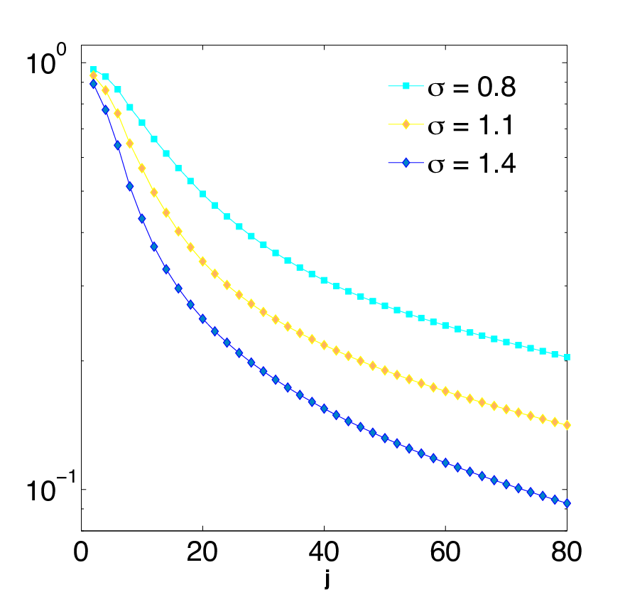
Figure 4 shows the time-evolution of the relative difference between the diffusion coefficients computed from (28), (28) and the mean square displacement computed from numerical simulations for various values of $\sigma$. This figures clearly supports the analytical computation presented in this Section.

References

- [1] R.P. Feynman and A.R. Hibbs. Quantum mechanics and path integrals. International Series in Pure and Applied Physics. McGraw-Hill Book Company, 1965.
- [2] Y. Aharonov, L. Davidovich, and N. Zagury. Quantum random walks. Phys. Rev. A, 48:1687, 1993.
- [3] D.A. Meyer. From quantum cellular automata to quantum lattice gases. J. Stat. Phys., 85, 1996.
- [4] H. Schmitz, R. Matjeschk, Ch. Schneider, J. Glueckert, M. Enderlein, T. Huber, and T. Schaetz. Quantum walk of a trapped ion in phase space. Phys. Rev. Lett., 103(090504):090504, August 2009.
- [5] F. Zähringer, G. Kirchmair, R. Gerritsma, E. Solano, R. Blatt, and C.F. Roos. Realization of a quantum walk with one and two trapped ions. Phys. Rev. Lett., 104:100503, 2010.
- [6] A. Schreiber, K.N. Cassemiro, A. Gábris V. Potoček, P.J.Mosley, E. Andersson, I. Jex, and Ch. Silberhorn. Photons walking the line. Phys. Rev. Lett., 104(050502):050502, 2010.
- [7] Michal Karski, Leonid Förster, Jai-Min Cho, Andreas Steffen, Wolfgang Alt, Dieter Meschede, and Artur Widera. Quantum walk in position space with single optically trapped atoms. Science, 325(5937):174–177, 2009.
- [8] Sansoni L, Sciarrino F, Vallone G, Mataloni P, Crespi A, Ramponi R, and Osellame R. Two-particle bosonic-fermionic quantum walk via 3d integrated photonics. Phys. Rev. Lett., 108(010502):010502, 2012.
- [9] B.C. Sanders, S.D. Bartlett, B. Tregenna, and P.L. Knight. Two-particle bosonic-fermionic quantum walk via 3d integrated photonics. Phys. Rev. A, 67:042305, 2003.
- [10] B. Perets, Y. Lahini, F. Pozzi, M. Sorel, R. Morandotti, and Y. Silberberg. Realization of quantum walks with negligible decoherence in waveguide lattices. Phys. Rev. Lett., 100:170506, 2008.
- [11] D. Giulini, E. Joos, C. Kiefer, J. Kupsch, I.-O. Stamatescu, and H.D. Zeh. Decoherence and the appearance of a Classical World in Quantum Theory. Springer-Verlag, Berlin, 1996.
- [12] A. Ambainis. Quantum walk algorithm for element distinctness. SIAM Journal on Computing, 37:210–239, 2007.
- [13] F. Magniez, J. Roland A. Nayak, and M. Santha. Search via quantum walk. SIAM Journal on Computing - Proceedings of the thirty-ninth annual ACM symposium on Theory of computing, New York, 2007. ACM.
- [14] C. Aslangul. Quantum dynamics of a particle with a spin-dependent velocity. Journal of Physics A: Mathematical and Theoretical, 38:1–16, 2005.
- [15] S. Bose. Quantum communication through an unmodulated spin chain. Phys. Rev. Lett., 91:207901, 2003.
- [16] D. Burgarth. Quantum state transfer with spin chains. University College London, PhD thesis, 2006.
- [17] S. Bose. Quantum communication through spin chain dynamics: an introductory overview. Contemp. Phys., 48(Issue 1):13 – 30, January 2007.
- [18] E. Collini, C.Y. Wong, K.E. Wilk, P.M.G. Curmi, P. Brumer, and G.D. Scholes. Nature, page 644.
- [19] G.S. Engel, T.R. Calhoun, R.L. Read, T.-K. Ahn, T. Manal, Y.-C. Cheng, R.E. Blankenship, and G. R. Fleming. Nature, page 782.
- [20] G. Di Molfetta and F. Debbasch. Discrete-time quantum walks: Continuous limit and symmetries. J. Math. Phys., 53:123302, 2012.
- [21] G. Di Molfetta, F. Debbasch, and M. Brachet. Quantum walks as massless dirac fermions in curved space. Phys. Rev. A, 88, 2013.
- [22] G. Di Molfetta, F. Debbasch, and M. Brachet. Quantum walks in artificial electric and gravitational fields. Phys. A, 397, 2014.
- [23] V. Kendon. Decoherence in quantum walks - a review. Math. Struct. in Comp. Sc., 17(6):1169–1220, 2007.
- [24] R. Vieira, E. P. M. Amorim, and G. Rigolin. Entangling power of disordered quantum walks. Phys. Rev. A, 89:042307, 2014.
- [25] Todd A. Brun, Hilary A. Carteret, and Andris Ambainis. Quantum to classical transition for random walks. Phys. Rev. Lett., 91:130602, Sep 2003.
- [26] A. Ahlbrecht, H. Vogts, A. H. Werner, and R. F. Werner. Asymptotic evolution of quantum walks with random coin. Journal of Mathematical Physics, 52(4), 2011.
- [27] Andre Ahlbrecht, Christopher Cedzich, Robert Matjeschk, VolkherB. Scholz, AlbertH. Werner, and ReinhardF. Werner. Asymptotic behavior of quantum walks with spatio-temporal coin fluctuations. Quantum Information Processing, 11(5):1219–1249, 2012.
- [28] Alain Joye. Random time-dependent quantum walks. Communications in Mathematical Physics, 307(1):65–100, 2011.
- [29] B. Kollar and M. Koniorczyk. Entropy rate of message sources driven by quantum walks. Phys. Rev. A, 89:022338, 2014.
- [30] Chaobin Liu and Nelson Petulante. On the von neumann entropy of certain quantum walks subject to decoherence. Mathematical Structures in Computer Science, 20:1099–1115, 12 2010.
- [31] C.M. Chandrasekhar, S. Banerjee, and R. Srikanth. Relationship between quantum walks and relativistic quantum mechanics. Phys. Rev. A, 81:062340, 2010.
- [32] G. Abal, R. Siri, A. Romanelli, and R. Donangelo. Quantum walk on the line: Entanglement and nonlocal initial conditions. Phys. Rev. A, 73:042302, Apr 2006.
- [33] Kota Chisaki, Norio Konno, Etsuo Segawa, and Yutaka Shikano. Crossovers induced by discrete-time quantum walks. Quantum Information & Computation, 11(9-10):741–760, 2011.
- [34] C. Navarrete-Benlloch, A. Perez, and Eugenio Roldan. Nonlinear optical galton board. Phys. Rev. A, 75:062333, 2010.
- [35] Hideaki Obuse and Norio Kawakami. Topological phases and delocalization of quantum walks in random environments. Physical Review B, 84(19):195139, 2011.
- [36] Yutaka Shikano, Tatsuaki Wada, and Junsei Horikawa. Discrete-time quantum walk with feed-forward quantum coin. Scientific reports, 4, 2014.
- [37] NV Prokof?ev and PCE Stamp. Decoherence and quantum walks: Anomalous diffusion and ballistic tails. Physical Review A, 74(2):020102, 2006.
- [38] A Schreiber, KN Cassemiro, V Potoček, A Gábris, I Jex, and Ch Silberhorn. Decoherence and disorder in quantum walks: From ballistic spread to localization. Physical review letters, 106(18):180403, 2011.
- [39] Norio Inui, Yoshinao Konishi, and Norio Konno. Localization of two-dimensional quantum walks. Physical Review A, 69(5):052323, 2004.
- [40] F. Debbasch. What is a mean gravitational field? Eur. Phys. J. B, 37(2):257–270, 2004.
- [41] A. J. Leggett, S. Chakravarty, A. T. Dorsey, Matthew P. A. Fisher, Anupam Garg, and W. Zwerger. Dynamics of the dissipative two-state system. Rev. Mod. Phys., 59:1–85, Jan 1987.
- [42] A.O. Caldeira and A.J. Leggett. Path integral approach to quantum brownian motion. Physica A: Statistical Mechanics and its Applications, 121(3):587 – 616, 1983.
- [43] F. Debbasch, K. Mallick, and J.P. Rivet. Relativistic Ornstein-Uhlenbeck process. J. Stat. Phys., 88:945, 1997.
- [44] C. Chevalier and F. Debbasch. Relativistic diffusions: a unifying approach. J. Math. Phys., 49:043303, 2008.
- [45] F. Debbasch, D. Espaze, and V. Foulonneau. Can diffusions propagate? J.Stat.Phys, 149:37–49, 2012.
- [46] G. Di Molfetta and F. Debbasch. Discrete-time quantum walks: Continuous limit in 1 + 1 and 1 + 2 dimension. J.Comp.Th.Nanosc., 10,7:1621–1625, 2012.
- [47] P. Arnault and F. Debbasch. Landau levels for discrete-time quantum walks in artificial magnetic fields. arXiv preprint, 1412.4337, 2014.
- [48] R.M. Wald. General Relativity. The University of Chicago Press, Chicago, 1984.