Spectral butterfly, mixed Dirac-Schrödinger fermion behavior and topological states in armchair uniaxial strained graphene
Abstract
An exact mapping of the tight-binding Hamiltonian for a graphene’s nanoribbon under any armchair uniaxial strain into an effective one-dimensional system is presented. As an application, for a periodic modulation we have found a gap opening at the Fermi level and a complex fractal spectrum, akin to the Hofstadter butterfly resulting from the Harper model. The latter can be explained by the commensurability or incommensurability nature of the resulting effective potential. When compared with the zig-zag uniaxial periodic strain, the spectrum shows much bigger gaps, although in general the states have a more extended nature. For a special critical value of the strain amplitude and wavelength, a gap is open. At this critical point, the electrons behave as relativistic Dirac femions in one direction, while in the other, a non-relativistic Schrödinger behavior is observed. Also, some topological states were observed which have the particularity of not being completly edge states since they present some amplitude in the bulk. However, these are edge states of the effective system due to a reduced dimensionality through decoupling. These states also present the fractal Chern beating observed recently in quasiperiodic systems.
pacs
73.22.Pr,71.23.Ft,03.65.Vf
I Introduction
Graphene is an amazing one-atom thick material. Its remarkable properties include high mobility, anomalous Hall quantum effect, Klein tunneling, lack of backscattering, etc [1]. Moreover, graphene possesses excellent mechanical properties, as for example the largest known elastic response interval (up to 25 of the lattice parameter [2]). The importance of this stems from the fact that it is possible to modify the electronic properties of graphene using elastic deformations, leading to a new field so called “straintronics” [3, 4, 5, 6]. For example, strain can modify electron-phonon coupling and even superconductivity [7]. In the literature, several approaches are used [5, 8, 9]. The most common one is to combine a tight-binding (TB) Hamiltonian with linear elasticity theory [8, 10, 11, 12]. Under this approach, high pseudo-magnetic fields appear, although assuming that the Dirac cone is not significantly modified [13]. However, for certain conditions that occurs experimentally, like in graphene grown on top of a crystal [14] or for rotated crystals [15], a gap can be opened at the Fermi level [16]. Such gaps are not obtained under the physical limit considered in the pseudo-magnetic field approach, although it has a paramount importance for technical applications. Using other approaches, it has been shown that the induced gap opening depends strongly upon the direction of the strain[3] and requires values as large as .
In a previous publication [16], we found a general method to map any zig-zag uniaxial strain into a one dimensional effective system. Such map opened the possibility to study strain from a new perspective. For example, we have proved that, in certain circumstances, periodic uniaxial strain produces a quasiperiodic behavior, due to the incommensurability of the effective resulting potential[16]. This resulted in a kind of modified Harper model [17]. The original Harper model leads to the Hofstadter butterfly [18], which arises in the problem of an electron in a lattice with an applied uniform magnetic field. At the same time, these kind of roughly ideas were experimentally confirmed for graphene on top of hexagonal boron nitride () as the rotational angle between the two hexagonal lattices was changed [15].
Unfortunately, in our previous work [16] we found that the gap sizes were very small and required strain’s amplitudes as large as of the interatomic distance. This was a little bit disappointing from the technological point of view, as well as for studying the topological properties [19]. Since it is known that graphene under uniaxial uniform arm-chair strain presents a bigger gap opening at the Fermi level than the zig-zag graphene [3], we decided to investigate the effects of a different kind of strain. As we will see throughout this paper, we found that it is possible to generate much bigger gaps using graphene’s nanoribbons under uniaxial armchair periodic elastic strain. Moreover, during this study we found an interesting effect at a critical point where a gap is open. At this point, the electrons have a mixed behavior. In one direction, a relativistic Dirac dynamics is followed, while in the other, a non-relativistic Schrödinger behavior is seen, i.e., the Dirac cone has a distorted cross section. As we will see, this results from a decreasing of the effective dimensionality due to strain. In fact, such behavior was theoretically anticipated by tuning ad hoc the graphene parameters [20, 21]. Although Montambaux and coworkers found since 2009 that bond pattern changes can result in a Dirac-Schröedinger behavior, there was not available an experimental set-up to produce such pattern. Here we prove that in fact, such possibility can be realized with the most simple oscillating strain. Our manuscript shows that armchair strain is needed to produce a transition to the Dirac-Schröedinger behavior, which is not observable using the zig-zag case.
This also opens the way to study interesting topological properties of the resulting one dimensional effective systems[19]. At this point, we would like to point out that many of the results presented in this manuscript are different from our previous work on zig-zag. In particular, the special kind of topological states found here are almost impossible to be observed in the zig-zag strain case because the gaps do not open or are very small for realistic values of strain.
Finally, it is important to discuss the possibility of having an experimental system with the proposed uniaxial stain. From this point of view, is clear that in order to have such strain, one needs to solve the elastic equations to derive the appropriate stress load. By using this kind of experimental set-up, it can be difficult to get the proposed uniaxial strain as we will discuss later on. A much better prospect is to grow graphene on top of another lattice, in which it has been demonstrated in some particular cases that the strain is uniaxial [14, 22]. Other systems that are suitable to observe the proposed effects are artificially made graphene superlatties [23, 24, 25], in which strain can be designed at will.
II Mapping of armchair uniaxial strain into an effective one dimensional system
When graphene is loaded with external forces, a strain pattern results. The new positions of the carbon atoms in the strained graphene are given by,
| (1) |
where are the unstrained coordinates of the carbon atoms. Notice that a critical step is to find the specific form of external forces to produce such strain pattern. Usually, this is found by inverting the elasticity Lamé equations [26]. In graphene, this inversion to find the force load pattern has been made in some cases, like in suspended graphene [27] or to produce an uniform pseudomagnetic field [28, 29]. Usually, such step is not a trivial task. An alternative is to use the finite-size method implemented in several available software tools.
We start with an armchair graphene nanoribbon, as shown in Fig. 1, with a uniaxial strain that produces an arm-chair strain. and
| (2) |
is the corresponding strain field, which here must depend only on . Although our approach can be applied
for a general strain of the form , here, for the sake
of simplicity, we will assume that in what follows.
Let us discuss briefly the possibility of building such strain experimentally, since there is a huge asymmetry in the types of strains that can be applied to graphene [30]: while the C-C bond length can be stretched by more than 20%, it is almost incompressible because it would always change bond angle instead of shrinking bond length by out-of-plane buckling. Therefore, it is extremely hard to apply compressive strain to graphene. However, there are several ways in which the proposed strain can be realized. First the proposed strain can be made without C-C compression if the lattice is already in a state of uniform expansion and then some bonds are further stretched. In that case, only the starting interatomic distances need to be changed and our results are basically renormalized. Second, even if we assume that there is buckling in the compressed C-C bond, the out-of-plane buckling can be modeled in a first approximation as a strain-field [31] Also, it has been proved that graphene grown over certain lattices has indeed uniaxial strain [22], and of course there is always the possibility of building a graphene superlattice with the proposed strain.
To obtain the electronic properties, we use a one orbital next-nearest neighbor tight binding Hamiltonian in a honeycomb lattice, given by [32],
| (3) |
where the sum over is taken for all sites of the deformed lattice. The vectors point to the three next-nearest neighbor of . For unstrained graphene where,
| (4) |
and y are the creation and annihilation operators of an electron at the lattice position .
In such model, the hopping integral depends upon the strain, since the overlap between graphene orbitals is modified as the inter-atomic distances change. This effect can be described by [31, 28],
| (5) |
where is the distance between two neighbors after
strain is applied. Here
, and corresponds to graphene without strain.
The unstrained bond length is denoted by , which will be taken as in what follows.
For any uniaxial armchair strain, we will prove that the Hamiltonian given by Eq. (3) can be mapped into an effective Hamiltonian made from two coupled chains, as indicated in Fig. 1. Let us bring such construction.
In non-strained armchair nanoribbons, the lattice can be thought as made from a periodic cell stacking [33]. Each cell has four non-equivalent atoms, as seen in Fig. 1. When uniaxial strain is applied, each cell has different strain. Thus, we introduce an index to label cells in the direction. The nanoribbon is now made from cells of four non-equivalent atoms with coordinates where , . Here, corresponds to the sub-lattice ( corresponds to sub-lattice ), as sketched in Fig. 1. For graphene without strain
| (6) |
and
| (7) |
On each of these sites, a strain field is applied, resulting in new positions,
| (8) |
where is a short hand notation for .
Within each chain, the nearest neighbor orbitals are coupled by the hopping parameter and have vanishing onsite energies.
For uniaxial strain, the symmetry along the -direction is not broken. Thus, the solution of the Schrödinger equation for the energy has the form , where is the wave vector in the -direction such that , is only function of , where and label the atoms along the arm-chair direction, as indicated in the Fig. 1. If we order the basis as , , …, , and ,, …, , , we obtain the following Schrödinger equation
| (9) |
where .
Now we label the atoms as in Fig. 1, this is, and . The sequences and can be written as where , labels the site number along the armchair path in the axis. Also, we observe that due to the uniaxial nature of the strain, several symmetries are found in the bonds, as well as , which allows to reduce the resulting Schrödinger equation .
Finally, the Hamiltonian is mapped into a new one without any reference to cells of four sites,
| (10) |
where , and , are the annihilation and creation operators in the lattices and respectively. This effective Hamiltonian describes two modulated chains coupled by bonds of strength and , as sketched out in Fig. 1, where are the values of the transfer integrals along the chains in the direction. They are obtained as follows.
First, we calculate the length between atoms after strain is applied,
| (11) |
In the present case, two different kinds of bond lengths are obtained,
| (12) |
where . and denote the and components of each of the vectors and
Thus, for odd values of ,
| (13) |
while for even values of ,
| (14) |
In order to compare with other works, it is interesting the case of small strain. Under such approximation, the hopping parameter between nearest neighbors along the chain is simplified a lot,
| (15) |
where it is understood that is the displacement of the -th atom along the vertical armchair path, i.e. . However, in the literature the most common approach is to use a linear approximation for the hopping parameter, given by,
| (16) |


Summarizing, Eq. (10) is an effective one dimensional Hamiltonian with effective hopping parameters given by equations (13) and (14). For small strain amplitude, Eqns. (13) and (14) are replaced by its linearized version Eq. (16). Such set of equations map any uniaxial armchair strain into a pair of coupled chains.
III Periodic armchair strain
To understand the rich physics involved in strain, let us know concentrate in the case of periodic strain, which arises when graphene is grown in top of a substrate with a different lattice parameter [14]. The simplest choice is to consider a sinusoidal kind of strain, similar to the observed pattern in graphene grown over iron [14]. This imposed oscillation contains three parameters, wavelength (controlled by the parameter ), amplitude (controlled by ) and phase (controlled by ). In order to simplify the resulting equations, we prefer to write the oscillating strain as,
| (17) |
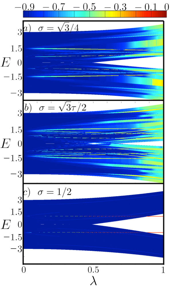
Figure 2 shows the complex spectrum of as a function of , obtained using fixed boundary conditions and by diagonalizing the resulting matrix for each value of . The calculation presented here was made for a width of atoms, and in Fig. 3 we present the resulting spectra for smaller sizes. As expected, the gaps are amplified for smaller sizes due to quantum confinement effects [33, 34], although there are fluctuations associated with the width, as happens with pure graphene nanoribbons[33]. Also, within our method it is possible to get bulk graphene by imposing periodic boundary conditions in the direction, as will be made for the case .
The most important feature of the resulting spectrum is its fractal nature, which is akin to the Hofstadter butterfly[18] which arises in the case of a lattice under a uniform magnetic field[17]. To have more information, we included color in Figure 2 to code the localization properties of the wavefunctions. They are studied by calculating the normalized participation ratio, defined as
| (18) |
The quantity estimates the occupied area by an electronic state [35]. For extended states (blue color in graphics), while it tends to be bigger when localization is presented (red color in the graphics). In the spectrum, it is clearly seen how different localizations coexist, making a very complex system in this respect.
To have a better understanding of the spectrum and its relationship with the Hofstadter buttery, it is useful to consider the small strain case. Using Eq. (16), the hopping integrals along the chains are given by,
| (19) |
We recognize that Eq. (19) corresponds to the transfer integrals of the off-diagonal Harper model[17], that produces a Hofstadter butterfly[18]. The main difference here is that we have an off-diagonal Harper ladder.
As in the Harper model, the fractal nature of the spectrum is given by the number theory properties of . When is a rational number, say , the effective one dimensional potential has a superperiod . Thus states have a Bloch nature. For irrational , the potential is quasiperiodic. Although the Bloch theorem is still valid, it does not provide any reduction of the problem since an infinite number of reciprocal space components are needed to generate the wave function [18]. This can generate a cascade of gaps or critical eigenstates [36]. Interestingly, in the Harper model, the gaps have a topological nature [36, 37, 38, 39, 40]. Moreover, since the problem of finding the solutions to a quasiperiodic potential is akin to the small divisor problem in dynamical systems [41], perturbation theory has a very limited value. A sequence of rational approximates or renormalization techniques are much better strategies to follow [41, 42, 43, 44].
It is also interesting to discuss the resulting bands as a function of , using different values of at a fixed lambda. In Fig. 4 we present the bands with the corresponding density of states (DOS) to the right. For we recover the graphene case, where the Dirac cones projections are seen at , resulting in a linear DOS at the Fermi level. However, for the three selected cases, , , and , the Dirac cones are completely destroyed. The DOS for the case suggests that the problem is akin to two uncoupled linear chains. As we will see, these two chains are not the ones that are observed to the right in Fig. 1, since and are never zero. These effective chains are in fact running in the direction, due to the fact that for some , we can have or even . Also, two edge states are observed at . These states are the remaining of the original Van Hove singularities that appear at the same energy for unstrained graphene. The other cases for irrational are spiky, as was also observed and explained in our work of zig-zag strain [16]. This is due to the quasiperiodic behavior of the resulting potential for irrational , which results in many nearly uncoupled linear chains of different widths[16]. Thus, the DOS are strikingly similar to those observed in narrow nanoribbons [45].

Conosider now how the spectrum changes with for a given . Fig.5 presents such evolution for fixed boundary conditions. The main result here is the big gap opening at the Fermi level for the different as grows. When compared with the zig-zag case [16], is clear that armchair strain is much more efficient to produce gaps, specially at the Fermi level. Also, the case shows two edge states at which have a topological nature, as will be discussed in a special section.
IV Half filling case : mixing Dirac and Schrödinger fermions
Of particular interest is the case , which for topological insulators is associated with half filling of the bands. For this case, the main interest is to know if a gap is open or not. We start by noting that the hopping parameter can be written, using Eq. (19), as
| (20) |
This result in a staggered ladder in which the unitary cell contains only four non-equivalent atoms. As a result, the effective Hamiltonian can be further reduced using the symmetry in the axis. For that end, the wave function can be written as,
| (21) |
where now . The corresponding spectrum is found by looking at the eigenvalues of the effective matrix Hamiltonian. whose solutions, in terms of the parameters , , and , are given by,
| (22) |
where,
| (23) |

The gap size can be found by minimizing the square of the energy in Eq. (22), since the bands are symmetric around . The momentums that produce a minimum are and , where . The resulting gap is given by,
| (24) |
and grows linearly with . This gap opening can be confirmed in Fig. 5. Notice however that the linear behavior is seen only near , mainly because Fig. 5 was made for the non-linearzed model.
Furthermore, at the critical point in which the spectrum changes from non-gapped to gapped, we obtained a very interesting behavior. In Fig. (6), we plot the dispersion relationship as a function of and . As one can see, at the Fermi level there is a kind of Dirac point at . However, it is not a cone. Instead, in the direction the behavior is linear, i.e., of the Dirac type, while in the direction behaves in a parabolic fashion, i.e., the fermions follow the usual Shrödinger behavior. For , and near the Dirac point, one can confirm such behavior by expanding Eq. (22) in series. In the direction () we find the Dirac behavior,
| (25) |
while in the direction () we find a Schrödinger behavior,
| (26) |
Thus, this highlights the paramount importance of the particular half-filling and half-amplitude critical point, in which the electron has a mixed Dirac and Schrödinger fermion dynamics, as seen in Fig. (6). The reason for this transition can be understood by looking at the limiting cases. For , the system is unstrained graphene in which electrons behave as Dirac fermions. At , for odd, resulting in a decoupled system in the direction. The system is thus made of two atom width nanoribbons spanning the direction. In this case, the particles follow a chain like behavior, i.e. of the Schrödinger type. As decreases, the parallel chains interact through a small interaction, as is suggested by the DOS that appear in Fig. 4 d), which corresponds to two linear chains. Thus, the critical point separates two regions of different effective dimensionality. One is mainly two dimensional while in the other, the propagation is nearly unidimensional. From a different point of view, this transition is due to the merging of Dirac cones, as was suggested in previous works by tuning ad hoc the transfer integrals [20, 21]. In Fig. 7, we present three stages of the dispersion relationship evolution near the critical point. Below , two Dirac cones are seen, which are merged at . Then a gap is open for . Notice that the mixing of Dirac-Schröedinger is not observable using the zig-zag case, since the effective chain does never have only two kinds of bonds [16].

V Topological states
As was discussed previously, in Fig. 4 d) and 5 c), two flat bands are seen at when . These two bands only appear when fixed boundary conditions are considered, since the energy dispersion for the bulk given by Eq. 22 does not present such states as seen in Fig. 8. Thus, these are edge states. It is well known that systems with band gaps and edge states can present non-trivial topological properties [46]. Here we decided to look at the behavior of the spectrum as a function of the phase in the potential, given by in Eq. (17).
In Fig. 8 we present the spectrum for the bulk and when fixed boundary conditions are included, as a function of the phase for and . As we can see, the edge states present a non-trivial topological behavior, since are absent in one of the gaps. We can track the behavior of the related states as seen in Fig. 8. For close to zero, the states are localized at the edges as expected, but surprisingly they also have amplitude near the center. However, this can be explained by observing that in this limit, we have almost chain decoupling. Thus, these states are edge states of the effective one dimensional system, which in fact it seems to be a very interesting phenomena. Furthermore, observe how the amplitudes are interlaced at the center, due to the symmetry of the problem. As the phase moves, these states eventually merges with the band edges, near , and present a non-localized nature. As shown in the figure, the pattern seems to be a sinusoidal with a long-wave modulation, which suggest that the Chern beating effect, originally observed and explained in quasiperiodic systems [19], is also present here.

VI Conclusions
In conclusion, we provided a general way to map any uniaxial armchair strain into an effective one-dimensional system. For the particular case of periodic strain, we obtained an spectrum akin to the Hofstadter butterfly. The armchair strain produces bigger gaps than the zigzag case. An analysis of the half filling case for the periodic strain, reveals a critical point for the opening of the gap. At this critical point, the fermions have a mixed behavior. In one direction they behave with a Dirac dynamics, while in the perpendicular one they follow a Schrödinger one. Such behavior arises as a consequence of a change in the effective dimensionality of the system. Also, we have observed some topological states due to strain. Interestingly, strain allows to have some ampiltude of the topological modes inside the bulk through a decoupling of the system. These states also present the phenomena of Chern beating observed in other quasiperiodic systems [19].
This opens the avenue for a whole set of new phenomena that seems to be realizable from an experimental point of view.
We thank Indu Satija and Maurice Oliva-Leyva for enlightening discussions and a critical
reading of the manuscript. This work was
supported by DGAPA-PAPIIT IN- project, and by DGTIC-NES center.
Pedro Roman-Taboada acknowledges support from CONACYT (Mexico).
References
- [1] K. S. Novoselov, A. K. Geim, S. V. Morozov, D. Jiang, Y. Zhang, S. V. Dubonos, I. V. Grigorieva, and A. A. Firsov, Science 306, 666 (2004), http://www.sciencemag.org/content/306/5696/666.full.pdf .
- [2] C. Lee, X. Wei, J. W. Kysar, and J. Hone, Science 321, 385 (2008), http://www.sciencemag.org/content/321/5887/385.full.pdf .
- [3] V. M. Pereira, A. H. Castro Neto, and N. M. R. Peres, Phys. Rev. B 80, 045401 (2009).
- [4] V. M. Pereira and A. H. Castro Neto, Phys. Rev. Lett. 103, 046801 (2009).
- [5] F. Guinea, Solid State Communications 152, 1437 (2012), exploring Graphene, Recent Research Advances.
- [6] D. Zhan, J. Yan, L. Lai, Z. Ni, L. Liu, and Z. Shen, Advanced Materials 24, 4055 (2012).
- [7] C. Si, Z. Liu, W. Duan, and F. Liu, Phys. Rev. Lett. 111, 196802 (2013).
- [8] H. Suzuura and T. Ando, Phys. Rev. B 65, 235412 (2002).
- [9] A. A. Pacheco Sanjuan, Z. Wang, H. P. PourImani, M. Vanevi, and S. Barraza-Lopez, Phys. Rev. B 89, 121403 (2014).
- [10] J. L. Mañes, Phys. Rev. B 76, 045430 (2007).
- [11] A. F. Morpurgo and F. Guinea, Phys. Rev. Lett. 97, 196804 (2006).
- [12] M. Vozmediano, M. Katsnelson, and F. Guinea, Physics Reports 496, 109 (2010).
- [13] M. Oliva-Leyva and G. G. Naumis, Phys. Rev. B 88, 085430 (2013).
- [14] N. A. Vinogradov, A. A. Zakharov, V. Kocevski, J. Rusz, K. A. Simonov, O. Eriksson, A. Mikkelsen, E. Lundgren, A. S. Vinogradov, N. Mårtensson, and A. B. Preobrajenski, Phys. Rev. Lett. 109, 026101 (2012).
- [15] C. R. Woods, L. Britnell, A. Eckmann, R. S. Ma, J. C. Lu, H. M. Guo, X. Lin, G. L. Yu, Y. Cao, R. V. Gorbachev, A. V. Kretinin, J. Park, L. A. Ponomarenko, M. I. Katsnelson, Y. Gornostyrev, K. Watanabe, T. Taniguchi, C. Casiraghi, H. J. Gao, A. K. Geim, and K. S. Novoselov, Nat Phys 10, 451 (2014).
- [16] G. G. Naumis and P. Roman-Taboada, Phys. Rev. B 89, 241404 (2014).
- [17] P. G. Harper, Proceedings of the Physical Society. Section A 68, 874 (1955).
- [18] D. R. Hofstadter, Phys. Rev. B 14, 2239 (1976).
- [19] I. I. Satija and G. G. Naumis, Phys. Rev. B 88, 054204 (2013).
- [20] L.-K. Lim, J.-N. Fuchs, and G. Montambaux, Phys. Rev. Lett. 108, 175303 (2012).
- [21] G. Montambaux, F. Piéchon, J.-N. Fuchs, and M. O. Goerbig, Phys. Rev. B 80, 153412 (2009).
- [22] G.-X. Ni, H.-Z. Yang, W. Ji, S.-J. Baeck, C.-T. Toh, J.-H. Ahn, V. M. Pereira, and B. Özyilmaz, Advanced Materials 26, 1081 (2014).
- [23] T. Uehlinger, G. Jotzu, M. Messer, D. Greif, W. Hofstetter, U. Bissbort, and T. Esslinger, Phys. Rev. Lett. 111, 185307 (2013).
- [24] U. Kuhl, S. Barkhofen, T. Tudorovskiy, H.-J. Stöckmann, T. Hossain, L. de Forges de Parny, and F. Mortessagne, Phys. Rev. B 82, 094308 (2010).
- [25] O. Peleg, G. Bartal, B. Freedman, O. Manela, M. Segev, and D. N. Christodoulides, Phys. Rev. Lett. 98, 103901 (2007).
- [26] A. Sommerfeld, Mechanics of deformable bodies: Lectures on theoretical physics, Lectures on theoretical physics (Academic Press, 1950).
- [27] J. C. Meyer, A. K. Geim, M. I. Katsnelson, K. S. Novoselov, T. J. Booth, and S. Roth, Nature 446, 60 (2007).
- [28] F. Guinea, M. I. Katsnelson, and A. K. Geim, Nat Phys 6, 30 (2010a).
- [29] F. Guinea, M. I. Katsnelson, and A. K. Geim, Nat Phys 6, 30 (2010b).
- [30] Y. Zhang and F. Liu, Applied Physics Letters 99, 241908 (2011).
- [31] R. M. Ribeiro, V. M. Pereira, N. M. R. Peres, P. R. Briddon, and A. H. C. Neto, New Journal of Physics 11, 115002 (2009).
- [32] W. Lu, P. Soukiassian, and J. Boeckl, MRS Bulletin 37, 1119 (2012).
- [33] A. Cresti, N. Nemec, B. Biel, G. Niebler, F. Triozon, G. Cuniberti, and S. Roche, Nano Research 1, 361 (2008).
- [34] G. G. Naumis, M. Terrones, H. Terrones, and L. M. Gaggero-Sager, Applied Physics Letters 95, 182104 (2009).
- [35] G. G. Naumis, Phys. Rev. B 76, 153403 (2007).
- [36] G. G. Naumis and F. López-Rodríguez, Physica B: Condensed Matter 403, 1755 (2008).
- [37] S. Ganeshan, K. Sun, and S. Das Sarma, Phys. Rev. Lett. 110, 180403 (2013).
- [38] M. Verbin, O. Zilberberg, Y. E. Kraus, Y. Lahini, and Y. Silberberg, Phys. Rev. Lett. 110, 076403 (2013).
- [39] Y. E. Kraus and O. Zilberberg, Phys. Rev. Lett. 109, 116404 (2012).
- [40] L.-J. Lang, X. Cai, and S. Chen, Phys. Rev. Lett. 108, 220401 (2012).
- [41] D. DiVincenzo and P. Steinhardt, Quasicrystals: The State of the Art, Series on directions in condensed matter physics (World Scientific, 1999).
- [42] G. G. Naumis and J. L. Aragón, Phys. Rev. B 54, 15079 (1996).
- [43] G. G. Naumis, Phys. Rev. B 59, 11315 (1999).
- [44] R. Nava, J. Tagüeña-Martínez, J. A. del Río, and G. G. Naumis, Journal of Physics: Condensed Matter 21, 155901 (2009).
- [45] K. Nakada, M. Fujita, G. Dresselhaus, and M. S. Dresselhaus, Phys. Rev. B 54, 17954 (1996).
- [46] X.-L. Qi and S.-C. Zhang, Rev. Mod. Phys. 83, 1057 (2011).