Interpolating between and
Abstract
We study the dimensional continuation of the sphere free energy in conformal field theories. In continuous dimension we define the quantity , where is the path integral of the Euclidean CFT on the -dimensional round sphere. smoothly interpolates between times the -anomaly coefficient in even , and times the sphere free energy in odd . We calculate in various examples of unitary CFT that can be continued to non-integer dimensions, including free theories, double-trace deformations at large , and perturbative fixed points in the expansion. For all these examples is positive, and it decreases under RG flow. Using perturbation theory in the coupling, we calculate in the Wilson-Fisher fixed point of the vector model in to order . We use this result to estimate the value of in the 3-dimensional Ising model, and find that it is only a few percent below of the free conformally coupled scalar field. We use similar methods to estimate the values for the Gross-Neveu model in and the model in . Finally, we carry out the dimensional continuation of interacting theories with 4 supercharges, for which we suggest that may be calculated exactly using an appropriate version of localization on . Our approach provides an interpolation between the -maximization in and the -maximization in .
1 Introduction and Summary
An important problem in -dimensional relativistic Quantum Field Theory (QFT) is to uncover general constraints on the Renormalization Group flow. When an RG trajectory connects a short-distance (UV) fixed point with a long-distance (IR) one, in some it has been possible to prove that a certain quantity, which characterizes the long-range degrees of freedom, is greater in the UV than in the IR. The first such inequality was proven in two space-time dimensions [1], i.e. for , and is commonly known as the theorem, since is the standard notation for the Virasoro central charge of a Conformal Field Theory. This quantity is also the Weyl anomaly coefficient and is proportional to the Stefan-Boltzmann constant of the theory at finite temperature. Soon after the seminal theorem [1] was established, a quest began for its generalization to . The Stefan-Boltzmann constant, , has been explored as a possible -function; it appears, however, that it does not generally decrease along RG flow unless the UV theory is free [2, 3, 4]. In , there are two Weyl anomaly coefficients, and it was conjectured [5] that the coefficient that multiplies the Euler density (in modern terminology it is called ) always decreases along RG flow. Over the years, this conjecture received support from studies of supersymmetric field theory where is determined by the symmetry [6], and the correct charges are fixed by the principle of -maximization [7]. A general proof of the -theorem has become available relatively recently [8, 9].
There is a considerable similarity between the theorems in and , since both of them concern the quantity that can be extracted from the free energy on the Euclidean sphere of radius : . In the Weyl anomaly coefficient may be extracted from the logarithmic term, . The same is true in , where the standard central charge is then defined via . Therefore, the two-dimensional -theorem is a particular example of a class of -theorems that may hold in all even dimensions, where is the coefficient of the dependence of the sphere free energy (alternatively, it is the Weyl anomaly coefficient which multiplies the Euler density). In odd dimensions, however, there is no Weyl anomaly, and therefore the appropriately regularized free energy is completely independent of the radius . Several years ago it was conjectured that, in odd dimensional RG flows, this regularized free energy satisfies inequalities similar to those satisfied by in even dimensions [10, 11, 12].11 1 For , this coincides with the much earlier work on the -theorem [13], where . In the most physically interesting case , a proof of the -theorem has been presented [14], relying on its exact relation with the entanglement entropy across a circle [15, 16].
The conjecture [11] that in was inspired by studies of RG flows with supersymmetry, where exact results are available via localization [17, 18, 19]. When the charges of a superconformal theory are not fixed by the superpotential, they are determined via the -maximization principle [18, 11, 20], which is analogous to the -maximization in . In this paper we will suggest an explicit connection between the - and -maximization by finding an appropriate maximization principle in continuous dimension for theories with four supercharges.
When the supersymmetric localization methods cannot be applied, the problem of calculating is in general difficult. Results are available for free CFTs and for large theories with double trace operators [12, 21, 22, 23, 24], but one is often interested in finding for non-supersymmetric CFTs that are strongly interacting and contain a small number of fields. For example, the most common second-order phase transition in 3-d statistical mechanics is in the universality class of the Ising model, which may be described by the Euclidean QFT of a real scalar field with a interaction.
A well-known generalization of the theory is to symmetric theory of real scalar fields , , with interaction . For small values of there are physical systems whose critical behavior is described by this QFT. When is sufficiently large, one can develop expansions for scaling dimensions of various operators using the generalized Hubbard-Stratonovich method [25, 26, 27, 28, 29, 30, 31, 32, 33]. Similarly, it is not hard to calculate in these CFTs, including the correction [12]
| (1.1) |
The correction of order has not been found yet. Even if it becomes available, this asymptotic expansion may not turn out to be very useful for low values of , since the available results for operator scaling dimensions exhibit rather poor convergence of the expansion.22 2 A more fundamental approach to the symmetric CFTs relies on the ideas of conformal bootstrap [34, 35, 36, 37], and recently it has led to precise numerical calculations of the operator scaling dimensions in three-dimensional CFT [38, 39, 40]. However, this approach has not yet shed light on the 3-sphere free energy . For example, [26, 25, 27]
| (1.2) | |||||
| (1.3) |
while the numerical values of these scaling dimensions for (the 3-d Ising model) are known to be and [41, 38, 39, 40]. Discarding the term in the anomalous dimension of , whose coefficient is very large, we obtain the approximation , which is twice as big as the actual value. The expansion is even less useful for estimating the dimension of in the 3-d Ising model.
Luckily, there exists another approximation scheme – the expansion [42] – that has led to better estimates for the IR scaling dimensions of composite operators. Instead of working directly in , one studies the physics as a function of the dimension . In the symmetric theory with the interaction, there is evidence that the IR critical behavior occurs for , and significant simplification occurs for where .33 3 One should keep in mind, however, that in non-integer dimensions even free theories are not unitary [43]. Then the IR stable fixed point of the Renormalization Group occurs for of order , so that a formal Wilson-Fisher expansion in may be developed [42]. The coefficients of the first few terms tend to fall off rapidly; for example, the anomalous dimension of is [44]
| (1.4) |
Setting provides rather precise approximations to the known experimental and numerical results for low values of [44, 42, 45, 46, 41, 38, 39, 40].44 4 One should note that the -expansion is only asymptotic, and extracting precise predictions from the higher orders in perturbation theory typically requires some resummation techniques, see e.g. [47] for a review.
This raises the hope that the expansion of the sphere free energy will also provide a good approximation. In this paper we will demonstrate, through a number of explicit calculations, that this is indeed the case. As a first step, in Section 2 we calculate it for the free conformally coupled scalar and massless fermion. We find that the quantity
| (1.5) |
is a smooth positive function of whose expansion indeed converges well. For odd integer , , in accord with the proposal of [12]. It also has a smooth limit as approaches an even integer, since the pole in is canceled by the zero of . Thus, the definition (1.5) proves to be very convenient for interpolating between the Weyl anomaly coefficients in even and the values in odd . In Section 3 we further demonstrate this by studying the large CFTs perturbed by double-trace operators in continuous dimension . The sphere free energies in such theories were studied in [21, 12, 23], and their dimensional continuation was carried out in [22, 24]. Using these results, we show that the quantity defined in (1.5) decreases for double-trace RG flow in all , provided the operator dimensions obey the unitarity bound. Studying other relevant deformations that cause a unitary UV CFT to flow to a unitary IR CFT, we consistently find that for all dimensions . This raises a tantalizing possibility that the -theorem in even integer dimensions and the -theorem in odd integer dimensions are special cases of the -theorem valid in continuous dimension.55 5 Conjecturing the -theorem may seem risky in view of the non-unitarity of theories in non-integer dimensions observed in [43]. However, the non-unitarity may not cause problems for positivity and monotonicity of .
In Section 4 we depart from the large limit and consider the specific example of Wilson-Fisher CFTs [42]. We perturb the CFT of free scalars by the operator , which is slightly relevant in . Using perturbative methods similar to those used in [5, 12] for slightly relevant operators on , we find the expansion of valid for all :
| (1.6) |
where is the free conformal scalar result (2.7). For the Ising model (), this expansion converges well and suggests that . This result, which is consistent with the -theorem, makes the smallest known -value for a unitary theory in . For comparison, we note that , the coefficient of the stress tensor 2-point function, is also known for the 3-d Ising model to be close to the free field value. The conformal bootstrap results give [38, 48].
In Section 5 we carry out the dimensional continuation of interacting theories with 4 supercharges. We keep the dimension of the anti-commuting directions of superspace fixed, while varying the number of spatial coordinates. In this fashion, theories with supersymmetry in are smoothly deformed into theories with SUSY in , and with SUSY in . In Section 5.1 we study the Wess-Zumino model with superpotential . This theory, which could be regarded as the simplest supersymmetric generalization of the Ising model, possesses a weakly coupled IR fixed point in . We develop the expansion using perturbation theory, and for compare it with the exact results from the localization on [17, 18, 19], finding excellent agreement. In the model describes the first member () of the series of superconformal minimal models with central charges [49]. Setting we find very good agreement with this exact result.
In Section 5.2 we argue that the supersymmetric localization on [17, 18, 19] can be generalized to continuous . For the Wess-Zumino models that contain only chiral multiplets, we propose an explicit function of their scaling dimensions, defined in (5.23) and (5.24), that has to be maximized in arbitrary . In our maximization reproduces the -maximization of [7], while in the -maximization of [18, 11, 20]. We compare the expansion for the model with the exact results as a function of , finding excellent agreement. In Section 5.3 we study a more complicated model with superfields and , , and the symmetric superpotential . In this model the scaling dimensions are not fixed by the superpotential, and we carry out the maximization, making contact with the results of [50] in , and of [51] in . We show that the -expansion of the anomalous dimension, found in [50], is in agreement with our proposal of maximization.
Among the motivations for studying the sphere partition functions for the -dimensional Euclidean CFTs where the dynamical fields transform in the vector representation of or , is their conjectured duality with the interacting higher spin theories in AdSd+1 [52, 53, 54, 55] (for a review, see [56]). While so far the duality has been tested in integer dimensions [57, 58, 59, 60, 61, 55], it may apply in continuous . In particular, as suggested in [52], it would be interesting to carry out the expansion in the Vasiliev higher spin theory [62, 63, 64, 65, 66, 67] and compare the results with those obtained in this paper.
2 for free fields
The eigenvalues and degeneracies of the Laplacian acting on fields of general spin on are known, and so it is not hard to compute for free fields in arbitrary dimension. In the case of conformally coupled scalars or massless fermions, a shortcut which yields a compact representation of the free energy is to use the known results for the change in under double-trace flows [21, 22, 23, 24] (this will be reviewed in Section 3 below). In this approach, one computes the determinant of the non-local kinetic operator of the auxiliary Hubbard-Stratonovich field, which is essentially the two-point function of a conformal primary of dimension . When is equal to the dimension of a free conformal field (i.e., for a scalar and for a spin 1/2 fermion), this two-point function is, as an operator, the inverse of the appropriate kinetic operator on , and hence their determinants are inverse of each other. Adopting this approach, one arrives at the following simple representations of for free conformal scalars and spin 1/2 fermions66 6 The mass-like term in the scalar kinetic operator arises from conformal coupling to the curvature, and we have set the radius to one.
| (2.1) | |||||
| (2.2) |
| (2.3) | |||||
| (2.4) |
Here is the trace of the identity in the Dirac matrices space. For convenience, we have defined to be independent of this factor so that it represents the value of a single Fermion component. For instance, in , as defined above corresponds to the contribution of a single Majorana fermion. In all examples discussed below, we will not need to continue to non-integer dimensions, but rather we will relate theories where is held fixed.
These expressions are valid for any and give a natural analytic continuation of to non-integer dimensions. It can be checked that in odd integer they reproduce the known values of for free fields given in Tables 1 and 2 of [12], e.g. in
| (2.5) |
On the other hand, near even , these expressions have simple poles whose coefficients reproduce the known -anomalies. For instance, in
| (2.6) |
which correspond respectively to the -anomaly coefficient of a real scalar and half of that of a Weyl fermion in (recall that in (2.3) we have divided by , so that in (2.3) corresponds to half the contribution of a Majorana or Weyl fermion).
The presence of the factor in the denominator of (2.1)-(2.3) suggests that it is natural to consider the quantity , so that
| (2.7) | |||
| (2.8) |
While oscillates between positive and negative values and has poles near even integer dimensions, one can see that is finite, smooth and positive in the continuous range of dimensions. In particular, since it is a finite quantity,77 7 Of course, there are power law divergences which are regulated away in dimensional regularization. is independent of the radius of . It smoothly interpolates between times the -values in odd , and times -anomaly coefficients in even . For example, in one gets
| (2.9) | |||||
| (2.10) | |||||
| (2.11) |
and similarly for the fermions. Plots of and for are given in Fig. 1. can be smoothly continued to , and for we find , which is the value of the quantity introduced in [13].

The smoothness of suggests that it is a useful quantity to consider in the framework of the -expansion. To further support this claim, in the rest of the paper we will present several examples of computations of in interacting theories that have a natural continuation to non-integer dimensions. As a first illustration that the -expansion of provides reasonable approximations, we can consider the explicit expansion of and in . A straightforward calculation starting from (2.7), (2.8) yields the result
| (2.12) | |||||
The numerical expansions are
| (2.13) | |||||
Setting in these expressions gives and , which are quite close to the exact values (2.5) in .
As an aside, we note that, since and are smooth functions of , it is not hard to develop their large expansions. Using the asymptotic expansion of the -function for large argument, we find
| (2.14) |
and
| (2.15) |
Note that at large this implies
| (2.16) |
which agrees with the structure found by a numerical interpolation of the -anomaly coefficients [68].
2.1 Free massive fields
It is straightforward to derive the value of for free massive fields for arbitrary . The eigenvalues and degeneracies for the scalar laplacian on the unit -dimensional sphere, , are
| (2.17) |
The free energy for a scalar of mass is then
| (2.18) |
The case corresponds to the conformally coupled scalar. Taking a derivative with respect to allows for a direct evaluation of the sum, and one gets
| (2.19) |
and so
| (2.20) |
where is the value corresponding to the conformal scalar (2.7). For example, in one obtains, in agreement with [12],
| (2.21) | ||||
In
| (2.22) |
Similarly, the eigenvalues and degeneracies for the Dirac operator on are
| (2.23) |
and so
| (2.24) |
This leads to
| (2.25) |
and finally
| (2.26) |
In one obtains [12],
| (2.27) | |||||
and in
| (2.28) |
3 Double-trace flows in large CFT’s
Let us a consider a CFT perturbed by the square of a primary scalar operator of dimension
| (3.1) |
We assume that the CFT has a large expansion, so that for large correlation functions factorize: . For example, the CFT could be a matrix-type theory and a single-trace operator, or we could consider a vector model whith being a bilinear in the fundamental fields.
A standard way to analyze the perturbed CFT is to introduce an auxiliary Hubbard-Stratonovich field
| (3.2) |
Then one can show that, for , the perturbed CFT flows to a large IR fixed point where has dimension [69, 21]. If , then the theory has a formal large UV fixed point, where has again dimension .
At the fixed point, the quadratic term in in (3.2) can be neglected, and one can develop a perturbation theory using the induced kinetic term for
| (3.3) |
where the subscript ’0’ denote correlators in the unperturbed CFT. Then, to leading order in the expansion, the change in the sphere free energy induced by the “double-trace” deformation is given by the determinant of the non-local kinetic operator for the field
| (3.4) |
where denotes the change in due to the perturbation. The two-point function of a primary of dimension on the sphere is fixed by conformal invariance to be (up to unimportant overall factors)
| (3.5) |
where is the chordal distance on . Expanding this two-point function in spherical harmonics, one ends up with the following expression for the determinant in (3.4) [21, 22]
| (3.6) |
where are the scalar degeneracies given in (2.17).88 8 Here we assume that the sum is evaluated using dimensional regularization, where the sum over degeneracies vanishes [22]. In this approach, the conformal anomaly arises as a pole in dimensional regularization close to even integer . Note that for , the eigenvalues coincide with the inverse of the eigenvalues for the conformally coupled laplacian (2.17), which implies that for this value of the formula (3.6) can be also used to obtain the value of for a free conformal scalar, as explained in the previous section.
Taking a derivative with respect to , performing the sum and integrating back yields the final answer [22]
| (3.7) | |||||
| (3.8) |
where we have used the identity . Equivalently, in terms of :
| (3.9) |
Note that setting and changing the overall sign (since this computes the determinant of the two-point function rather than the kinetic operator), this indeed agrees with (2.7).
Similarly, one can consider a CFT perturbed by the square of a spin 1/2 operator of dimension . Introducing a fermionic Hubbard-Stratonivich field and computing the determinant of its induced kinetic operator, one arrives at the final result [23, 24]
| (3.10) |
Setting and changing overall sign, this reproduces the free fermion result in (2.8).
A simple example of such double-trace flow is provided by the symmetric scalar field theory with quartic interaction
| (3.11) |
For , this theory flows to the well-known Wilson-Fisher IR fixed point, which can be studied in the framework of the -expansion in . At large , the quartic interaction term can be viewed as a double-trace deformation of the type described above, with , and it is straightforward to compute using eq. (3.9). For , one obtains [12]
| (3.12) |
It is known that the UV fixed points of the non-linear sigma model in provide an alternative description of the same critical CFT. The 3d -theorem then implies that the critical CFT should satisfy
| (3.13) |
where the right inequality comes from the description as IR fixed point of the quartic theory, and the left one from the non-linear sigma model point of view. Equivalently, this implies in that , which is indeed seen to be true from eq. (2.5) and (3.12). A natural question is whether the quantity also satisfies in continuous dimensions. This would imply by the same logic that . Using (3.9) and (2.7), one can verify that this is indeed true in the whole range . This provides some evidence for the validity of the theorem in continuous .
For later reference, let us also work out the explicit expansion of . Using (3.9), a short calculation yields the result
| (3.14) |
Setting , this yields the estimate , while the exact result (3.12) is . Including a few more orders in the -expansion quickly improves the agreement with the exact answer.
The quartic theory (3.11) was also recently reconsidered in the range . In , the model has a formal UV fixed point at negative coupling. It was recently proposed that the same interacting CFT can be described as the IR fixed point of a symmetric cubic theory with scalars in , which is unitary for sufficiently large [70]. Then, the condition implies in that , or, in terms of
| (3.15) |
This was checked to be true in [70]. Using (3.9) and (2.7), we have verified that in fact it holds in the whole range . This provides additional evidence for the validity of the theorem in continuous .
Let us also work out the expansion of near six dimensions:
| (3.16) |
The leading contribution is indeed equal to times the anomaly coefficient of a free massless scalar in (see (2.11)), in precise agreement with the description of the critical CFT in terms of the cubic theory in . Subtracting the contribution of one free scalar, we get
| (3.17) |
This subtraction will allow for a more direct comparison with the perturbative calculation for the cubic scalar theory in in the next section.
Another interesting CFT example is the Gross-Neveu model [71] in the dimension range
| (3.18) |
where are Dirac fermions. This theory has perturbative UV fixed points in . At large , one can study these fixed points using the Hubbard-Stratonovich approach described above, in the whole range (for , the fixed points become non unitary). Remarkably, it was found that this critical fermionic theory has an alternative, “UV complete”, description in terms of the IR fixed points of a Gross-Neveu-Yukawa (GNY) model in [72, 73, 74]. The GNY model includes an extra propagating scalar field interacting with the fermions via the Yukawa interactions
| (3.19) |
The existence of the two alternative descriptions of the same CFT imply that, if , then
| (3.20) |
At large , in terms of defined in (3.9), this implies
| (3.21) |
Note that in this case , which is the dimension of the operator in the free CFT. This inequality was checked to be true in [12, 70], where . Using the dimensionally continued results (3.9) and (2.7), we have verified that it holds in the full range (and it is violated for , where the theory becomes non-unitary). Finally, since it will be useful in the next section, let us quote the explicit expansion of near four dimensions. Setting and expanding for small , one finds
| (3.22) |
The first two terms are the same as the free scalar result in , which is a nice test that near four dimensions one gets an extra propagating scalar, as in (3.19). This suggests that it is useful to consider the difference
| (3.23) |
This result will be compared with a perturbative calculation in the GNY model in the next section.
4 Weakly coupled fixed points in the -expansion
4.1 scalar theory in and the Ising model
The action for the quartic scalar field theory in is
| (4.1) | ||||
Here we have written the first line in terms of bare fields and coupling, and the second line in terms of renormalized fields and dimensionless coupling , with the renormalization scale. The counterterms and are known up to five loop order in dimensional regularization [75, 47]. The leading terms read
| (4.2) |
The corresponding -function in is [75, 47]
| (4.3) |
Then, one can see that there is a perturbative IR fixed point at a critical coupling given by
| (4.4) |
For and , this fixed point describes the Ising model in .
We now want to conformally map the theory to and compute the sphere free energy at the IR fixed point. The action of the model on the sphere is the same as (4.1), provided we covariantize it and add the conformal coupling term . In addition, one should include a renormalization of the conformal coupling parameter as well as pure curvature counterterms, which are needed to make the free energy finite starting at order [76, 77]. The counterterms , (and hence the -function and fixed point coupling ) are fixed by the flat space UV divergences and so we can still use (4.2) when working on the sphere.
The free energy to cubic order in is given by
| (4.5) | |||||
| (4.6) |
where , and . Here we have used the fact that , being a one-point function in a (free) CFT, vanishes. Note that the wave function renormalization does not in fact enter at this order (it will affect the order and higher). The two and three point functions of the free theory on the sphere read
| (4.7) | |||
where is the chordal distance. In the stereographic coordinates where the metric of with radius is , it reads
| (4.8) |
Let us recall the integrals [5, 12]
| (4.9) | |||
In the present case, we have , and so
| (4.10) | ||||
Setting , we obtain the expansions
| (4.11) | |||
| (4.12) |
Inserting these into (4.10), and using the explicit form of the counterterm (4.2), one can verify that the pole in is cancelled. This agrees with the results of [77, 76], where it was found that the additional curvature counterterms are not needed to cancel divergences before order . If we remove the dimensional regulator, then we get the result
| (4.13) |
from which we find
| (4.14) |
which agrees with known results for the integrated trace of the stress tensor in the theory [78]. We also note that the Callan-Symanzik equation is satisfied to this order (here is the 4d beta-function, i.e. eq. (4.3) with ).
On the other hand, in the case of the fixed points which is our main interest here, using (4.10), (4.12), and the expression for the critical coupling given in (4.4), we obtain the result99 9 This result also includes the effect of the Euler density counterterm [76, 77]. This counterterm enters the renormalization process at order , but after setting its renormalized coefficient to the zero of its beta function in , it produces an additional finite contribution to equal to . Adding this term to (4.10), one obtains the result (4.15). This corrects the corresponding formula in earlier versions of this paper, where the effect of the curvature term was not included. The curvature contribution will be discussed in more detail in [79].
| (4.15) |
Note that the term proportional to has cancelled out, consistently with conformal invariance of the fixed point theory (we do not have a conformal anomaly in ). Equivalently, in terms of , we thus have (1.6). A non-trivial test of this result comes from comparing with the double-trace formulae at large . Indeed, expanding (1.6) to leading order at large , we find agreement with the expansion (3.14) in .
We can now use (1.6) to obtain an estimate for in the 3d Ising model. Setting and , and using the expansion (2.13) for , we obtain1010 10 Since we have found the effects of interaction up to , for consistency we keep only the terms up to in the expansion of .
| (4.16) |
Note that the correction in (1.6) due to interactions is quite small. Recalling that, in , (see (2.5)), our result implies
| (4.17) |
Thus, the value of the 3d Ising model appears to be rather close to the free field value. This is in line with the recent bootstrap results for the stress tensor two point function coefficient , which yield [38, 48]. The fact that is consistent with the -theorem in . It is natural to propose that is the lowest possible value of in a unitary 3-dimensional CFT.
We can further use (1.6) to study the ratio for . As is increased, this ratio first decreases slightly, attaining a minimum of for . After that it begins to increase, and for large it approaches 1. A plot of the ratio as a function of continuous is shown in Fig. 2. Interestingly, the same qualitative behavior as a function of (a slight decrease followed by increase) is also found in conformal bootstrap calculations of [39]. The non-monotonicity in can also be seen in the behavior of , which increases slightly from to and then begins to fall [39].

We may consider further decreasing and comparing with the known exact results in . The fixed point, i.e. the theory, is expected to be continuously connected to the 2-d Ising model [80], which has central charge known to be the smallest possible for a unitary 2-d CFT. The fixed point should connect with the theory of a compact scalar field, which has . For the theory is the non-linear sigma model which is not conformal. In terms of , . If we take our result (1.6) in , set , , and divide by the free scalar contribution , we obtain
| (4.18) |
which is not too far off the expected value of , considering that we only have the first few orders in the expansion. Similarly, setting , in (1.6) we find ; this is not far off the exact result . A plot of the -expansion prediction for as a function of for , normalized by the free scalar result is given in Fig. 3.

Let us mention that another possible approach is to dimensionally continue the ratio , instead of itself. From our result (4.15) in , we have
| (4.19) |
Expanding to quartic order in , and then setting , , yields
| (4.20) |
which is slightly different from our estimate (4.17) above. This is not surprising, given that this approach essentially involves a partial resummation of (4.15). Clearly, higher orders in the expansion, potentially coupled with some kind of resummation technique, may be necessary to obtain a more precise estimate of . Nevertheless, we believe that the conclusion that is a few percent below the free scalar value is robust.
4.2 Gross-Neveu-Yukawa model
Another interesting example of weakly coupled fixed points in is provided by the GNY model (3.19). The one-loop -functions for the renormalized couplings , are [74]
| (4.21) | ||||
where , and is the number of Dirac fermions (i.e., the model has a global symmetry). There is a stable IR fixed point at the critical couplings
| (4.22) | ||||
The corrections to the critical couplings and to the operator anomalous dimensions were found in [81] using the two-loop beta functions.
The calculation of the sphere free-energy at the fixed points follows the same step as in the previous section. To leading order, only the Yukawa coupling contributes, since at the fixed point , . We have
| (4.23) |
and so
| (4.24) |
Note that to this order we do not need to worry about the contribution of the counterterms (they will cancel the poles coming from higher order diagrams). Using (4.9), and inserting the fixed point value of the coupling constant, we get
| (4.25) |
or, in terms of
| (4.26) |
We see that at large this precisely agrees precisely with the double-trace result (3.23). Note also that the sign of the correction due to interactions is negative, in agreement with the expectation that . Expanding the free field results and to order , we find
| (4.27) |
Now setting , we obtain an estimate for the 3d critical Gross-Neveu model
| (4.28) |
For the case of the Gross-Neveu model, we should set .1111 11 If we instead define the dimensional continuation so that the number of degrees of freedom is kept fixed, then the lowest possible value is , corresponding to two Dirac fermions in . Then, we get the estimate . The corresponding free field value is
| (4.29) |
so that
| (4.30) |
4.3 Cubic scalar theory in
Let us now consider the symmetric cubic scalar field theory in
| (4.31) |
Again, we omit the explicit counterterms, as we will only do a leading order computation of the free energy.
The one-loop -functions for the renormalized couplings are [70]
| (4.32) | ||||
For , these have real zeroes corresponding to unitary IR stable fixed points. The solution for the critical couplings has the form
| (4.33) |
where is the solution to the cubic equation
| (4.34) |
with large asymptotics .1212 12 The other two solutions have asymptotics and they are not IR stable for generic . As is reduced, this real solution disappears at the critical value of where the discriminant of the cubic equation (4.34) vanishes; this happens for [70].1313 13 Higher loop corrections show that the value of this critical is significantly reduced as is increased [82].
It is not difficult to derive the large expansion of the critical couplings to any desired order. The first few terms read [70]
| (4.35) | ||||
Now, let us calculate the first correction to the sphere free energy in . We just need the two-point functions in the free theory
| (4.36) | ||||
and so we get
| (4.37) |
Using (4.9) and expanding to leading order in , we get
| (4.38) |
where are the fixed point couplings (4.33). Note that the change in is positive in this case. However, in terms of , we have
| (4.39) |
which is consistent with (the reason for the change of sign is simply that in ). Using the large expressions (4.35) for the fixed point couplings, it is also easy to check that this result agrees as expected with the double-trace formula (3.17).
5 SUSY theories: comparing localization and -expansion
5.1 The Wess-Zumino model with cubic superpotential in
It is known that the usual dimensional regularization is inconsistent with supersymmetry, since it breaks the balance between bosonic and fermionic degrees of freedom. However, a variant of dimensional regularization, known as dimensional reduction scheme [83, 84] is widely used in loop calculations in supersymmetric theories.1414 14 This scheme is also used in loop calculations in supersymmetric Chern-Simons matter theories in (see e.g. [85]), for which the usual dimensional regularization cannot be used due to the presence of the Chern-Simons term. In this regularization scheme, all tensor and spinor manipulations are done in the fixed integer space-time dimension, and at the end the loop integrals are continued to non-integer dimensions. This procedure preserves supersymmetry and it is believed to be a consistent regularization technique in supersymmetric field theories. While this scheme is typically employed to regulate loop calculations near a given integer dimension, here we will use it to connect theories with four supercharges in , in the spirit of the Wilson-Fisher -expansion. In this way, we will connect Wess-Zumino models in , to models in and models in .
As an explicit simple example, let us consider the Wess-Zumino model with a cubic superpotential for a chiral superfield :
| (5.1) |
This theory has classically marginal interactions in , and the corresponding function is known to four loop order [86, 87, 88, 89]. Due to the non-renormalization of the superpotential vertex [90, 83], the -function is completely determined by the wavefunction renormalization of
| (5.2) |
where is the -function in , whose first few orders read
| (5.3) |
When we continue the model to , the -function becomes simply
| (5.4) |
Then, we see that in there is a perturbative IR fixed point given by
| (5.5) |
This is a supersymmetric version of the Wilson-Fisher fixed point for the quartic scalar field theory in . In , it describes the IR fixed point of the Wess-Zumino model with cubic superpotential (see e.g. [91]). Note that (5.2) completely determines the dimension of at the fixed point, where . Then, at the IR fixed point we find
| (5.6) |
or, writing
| (5.7) |
In particular, in this corresponds to the free field dimension , and in it gives at the interacting IR fixed point [91]. Another way to derive the exact dimension (5.7) is to note that, in all dimensions the superpotential must have the charge equal to , so that . Continuing the BPS condition from integer to real , we then recover (5.7).
In , the sphere free energy of any supersymmetric field theory can be computed exactly using the supersymmetric localization [17, 18, 19]. Introducing the function [18]
| (5.8) | ||||
the free energy of the model with at the fixed point is given by
| (5.9) |
where we used the fact that the conformal dimension in the IR is fixed by the superpotential. This may be compared with the value of for the free chiral multiplet, . Therefore,
| (5.10) |
in agreement with the -theorem.
To test the validity of the -expansion, let us now try to compute perturbatively the sphere free energy of this model in . The calculation is very similar to the one for the GNY model described in Section 4.2. In components, the Lagrangian of the Wess-Zumino model reads [87]
| (5.11) |
where and are a real scalar and pseudo-scalar, and a Majorana fermion (this has two propagating degrees of freedom in , the same as a Dirac fermion in ). To leading order, the only contribution to the sphere free energy comes from the Yukawa interactions. Using the integrals defined in (4.9), we thus get
| (5.12) |
Note that a factor of 2 comes from the fact that the fermions are Majorana (so that there are non-zero Wick contractions and ), and an additional factor of 2 takes into account the two Yukawa couplings and . Finally, the factor is the trace of identity in the gamma matrices space, which should be set to according to the rules of dimensional reduction. Then, plugging in the critical coupling (5.5), expanding to leading order in and inserting a factor of , we get the result for
| (5.13) |
The free field contribution corresponds to a free conformal chiral superfield, for which we get (see eq. (2.13))
| (5.14) |
Then, we obtain the prediction to quadratic order in :
| (5.15) |
In , this gives
| (5.16) |
which is within 1% of the exact localization result (5.9)! Thus, the -expansion seems to be a remarkably good approximation (at least in this supersymmetric example), given that we have only performed a leading order calculation in .
It is also interesting to consider the continuation of the model to . In this case, the IR fixed point corresponds to the SCFT with cubic superpotential, which has and central charge . This is the first member, , of the superconformal minimal models in ; these theories have superpotentials and central charges [49]. Setting in our result (5.15), we obtain
| (5.17) |
corresponding to central charge . This approximation from the expansion is again remarkably close to the exact result .
5.2 Interpolating -maximization
In this section we propose a natural extension of the localization on [17, 18, 19] that can be applied to any Wess-Zumino type model with four supercharges on , . As we will show below, our proposal smoothly interpolates between the -maximization [7] in , and the -maximization [18, 11, 20] in .
We start by observing that the function (5.8) appearing in the 3d localization for supersymmetric theories has a simple origin. It can be obtained from the one-loop determinants on of free massive scalars and fermions. Indeed, the supersymmetric Lagrangian for a free chiral multiplet with non-canonical dimension is given by [18, 19, 92]
| (5.18) |
where we have assumed that there is no vector multiplet in the theory, and we have set the radius of the sphere to one. Adding a superpotential to the theory does not change the value of the localized partition function, except for constraining the allowed values of the -charges. Then, each chiral multiplet with trial dimension contribute to the partition function a factor
| (5.19) |
The relevant functional determinants can be obtained from the results (2.21) and (2.27) for free massive fields, and correspond to the free energy contribution
| (5.20) |
where we recall that the value of the scalar mass was defined in (2.18) as the deviation from conformal coupling, and the factor of 2 is because the 3d chiral superfield contains a complex scalar and a Dirac fermion.
This suggests a natural generalization of the 3d localization to non-integer . To a given chiral superfield with trial dimension , or equivalently trial -charge , we associate the function
| (5.21) |
where and are the -values of free massive fields given in (2.20) and (2.26). The value of the masses above are such that they reduce to (5.20) for , and for the canonical dimension they correspond to the usual conformal coupling in dimension . The function can be given a more compact representation in terms of its derivative with respect to . Using the results in Section 2.1, we find
| (5.22) |
Integrating this equation with the boundary condition that must equal the contribution of a free conformal chiral multiplet, (5.14), we find
| (5.23) |
By comparing (5.22) and (5.23) to (5.8), it is straightforward to verify that for . Our proposal can be then stated as follows. For a theory with four supercharges including several chiral superfields (and restricting for the time being to theories without gauge fields), the exact value of is given by
| (5.24) |
where the trial dimensions are determined by maximizing , under the constraint that the superpotential has exact -charge 2. In , this reproduces the result of [18] by construction. Let us show that in this is equivalent to the -maximization of [7]. Specializing (5.23) to , we obtain
| (5.25) | |||||
| (5.26) |
where in the second step we have used . This is indeed the correct expression for the -anomaly of a chiral superfield as a function of the -charge of the scalar field [6] (recall that in our conventions imply that ). Thus, the maximization of (5.24) indeed smoothly connects the 4d -maximization and 3d -maximization.
It is also worth noting that in our proposal (5.24) correctly reproduces the central charges of the superconformal minimal models. In , from (5.23) and (5.22) we get
| (5.27) |
Thus, we find that the central charge is given by
| (5.28) |
in agreement with [49]. For example, for the superconformal model with , the dimension of is . So we obtain
| (5.29) |
which indeed corresponds to the correct central charge [49].
A non-trivial test of (5.24) can be obtained by comparing with the direct perturbative calculation for the model in performed in the previous section. Setting and , and expanding in powers of , (5.23) and (5.24) give
| (5.30) |
The leading order term indeed precisely reproduces our perturbative result (5.13). To further test the correctness of our localization proposal, it would be interesting to match the subleading corrections by a direct Feynman diagram calculation in . It is also interesting to compare the exact localization prediction (5.24) in to the -expansion. In Fig. 4, we plot the exact prediction for normalized by the value for a free chiral superfield, and compare it to the -expansion: remarkably, keeping only up to order already provides a very good approximation of the exact result in the whole range .
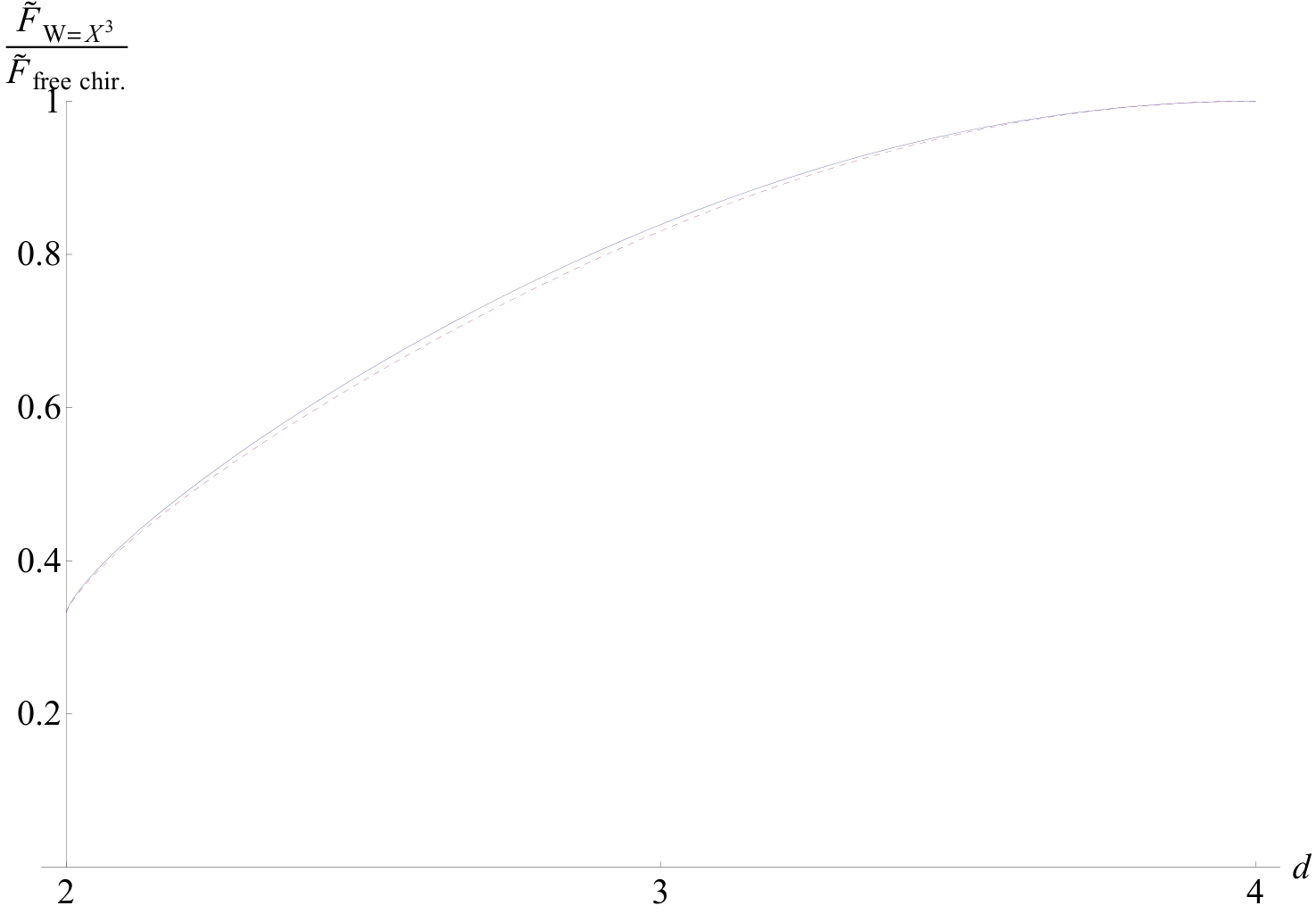
We may also consider the expansion of models which have classically marginal interactions in . The simplest such theory is the model with quartic superpotential . This model is IR free in , but it is expected to have non-trivial IR fixed points in . In it becomes the second member, , of the superconformal discrete series with central charges [49]. This model with may be regarded as a supersymmetric version of the tricritical Ising model. It is straightforward to derive for this model in . The dimension in the IR is fixed to be . Inserting this value in (5.23) and expanding in , we obtain the prediction
| (5.31) |
where the free chiral superfield contribution in is
| (5.32) |
It would be interesting to reproduce (5.31) from a direct perturbative calculation in . Setting in (5.31) and including the free field contribution expanded to order , we obtain the estimate in , corresponding to which is close to the exact value . Thus, we again see that the first few orders of the expansion provide rather good approximations to the exact answers.
5.3 An example with symmetry
So far, we have discussed examples where the charges are completely fixed by the superpotential. As an example where the -maximization is needed to fix the charges, let us consider the model with chiral superfields and symmetric superpotential
| (5.33) |
This model has classically marginal interactions in , and its RG analysis in was carried out in [50].1515 15 Note that from the RG point of view it would be natural to add the term to the superpotential, which is also classically marginal in and consistent with the symmetry. However, we note that the theory with superpotential (5.33) has an additional global symmetry under which can be assigned charge and charge . This symmetry ensures that the term is not generated. Equivalently, one can also explicitly see that the beta function vanishes at . This follows from general non-renormalization properties of the Wess-Zumino models in , which imply , analogously to (5.2). The -function and anomalous dimensions for this model are known up to the four loop order [93]. The first few orders read
| (5.34) | |||
| (5.35) | |||
In the theory is IR free, while in one can see that there is a perturbative IR fixed point with
| (5.36) |
This is continuously connected to the non-trivial IR fixed point of the 3d model with the same superpotential (this model was recently used in [51] to provide a counterexample to a potential theorem in ). Note that the anomalous dimensions and -function in (5.35) are related by , analogously to (5.2). This implies that at the IR fixed point the conformal dimensions are constrained by
| (5.37) |
This is equivalent to the condition that the -charge of the superpotential equals .
As a test of the -extremization procedure, we can use it to derive the conformal dimensions and in , and compare the result with the RG analysis. Given the constraint (5.37), the exact is given by
| (5.38) |
where we used (5.37), and the value of should be determined by extremizing . Using (5.22), we obtain
| (5.39) |
Setting
| (5.40) |
and expanding in powers of , we can easily solve the equation to obtain
| (5.41) |
One can check that this result precisely agrees with the one obtained from the RG analysis [50, 93] (see eq. (5.35)) providing a non-trivial test of our proposal. Once the conformal dimensions in the IR are known, one can plug them back in (5.23) to obtain the exact . Using (5.41), we obtain in
| (5.42) |
Expanding to order , this gives for and the values , which are very close to the exact 3d results found in [51].
It is also interesting to solve (5.39) at large and fixed . Setting , and solving perturbatively at large , we obtain
| (5.43) | ||||
where . This exactly matches the result of [50] obtained by large methods. In , it gives
| (5.44) |
in agreement with [51]. By plugging (5.43) into (5.23), one can also obtain in principle the large expansion of for any . In , this can be seen to reproduce the large expansion of (5.42) as expected. In , the result can be obtained directly from . Using (5.44), one gets [51]
| (5.45) |
Note that in the -maximization procedure cannot be carried out, since is linear in (see eq. (5.27)). This suggests that the superpotential (5.33) does not give a superconformal theory in , unless the conformal dimensions are completely fixed by and its symmetries. Consider, for instance the series of theories which have with and [49]. We note that there is no theory with , where the superpotential does not fix the dimensions. When the superpotential has both terms, then the dimensions are fixed to and . The correct central charge then follows from (5.28). We also note that the theory has a superpotential that is marginal in , so it can be studied using the expansion.
Another interesting theory is the case of (5.33), where by a change of variables the theory is equivalent to the model with superpotential . This model is well-known in because it is related by the mirror symmetry to supersymmetric QED with one flavor [91]. In general , the conformal dimensions are fixed to be
| (5.46) |
Indeed, note that all the anomalous dimensions in (5.41) vanish for , except for the term which is linear in and, therefore, linear in . The exact for this model is then simply
| (5.47) |
In , this corresponds to a superconformal model with , or central charge .
Acknowledgments
We thank L. Fei, S. Pufu, B. Safdi, G. Tarnopolsky and I. Yaakov for useful discussions. The work of SG was supported in part by the US NSF under Grant No. PHY-1318681. The work of IRK was supported in part by the US NSF under Grant No. PHY-1314198.
References
- [1] A. B. Zamolodchikov, “Irreversibility of the Flux of the Renormalization Group in a 2D Field Theory,” JETP Lett. 43 (1986) 730–732.
- [2] A. Castro Neto and E. H. Fradkin, “The Thermodynamics of quantum systems and generalizations of Zamolodchikov’s C theorem,” Nucl.Phys. B400 (1993) 525–546, cond-mat/9301009.
- [3] S. Sachdev, “Polylogarithm identities in a conformal field theory in three-dimensions,” Phys.Lett. B309 (1993) 285–288, hep-th/9305131.
- [4] T. Appelquist, A. G. Cohen, and M. Schmaltz, “A New constraint on strongly coupled gauge theories,” Phys.Rev. D60 (1999) 045003, hep-th/9901109.
- [5] J. L. Cardy, “Is There a c Theorem in Four-Dimensions?,” Phys.Lett. B215 (1988) 749–752.
- [6] D. Anselmi, D. Freedman, M. T. Grisaru, and A. Johansen, “Nonperturbative formulas for central functions of supersymmetric gauge theories,” Nucl.Phys. B526 (1998) 543–571, hep-th/9708042.
- [7] K. A. Intriligator and B. Wecht, “The Exact superconformal R symmetry maximizes a,” Nucl.Phys. B667 (2003) 183–200, hep-th/0304128.
- [8] Z. Komargodski and A. Schwimmer, “On Renormalization Group Flows in Four Dimensions,” JHEP 1112 (2011) 099, 1107.3987.
- [9] Z. Komargodski, “The Constraints of Conformal Symmetry on RG Flows,” JHEP 1207 (2012) 069, 1112.4538.
- [10] R. C. Myers and A. Sinha, “Seeing a C-Theorem with Holography,” Phys. Rev. D82 (2010) 046006, 1006.1263.
- [11] D. L. Jafferis, I. R. Klebanov, S. S. Pufu, and B. R. Safdi, “Towards the F-Theorem: Field Theories on the Three- Sphere,” JHEP 06 (2011) 102, 1103.1181.
- [12] I. R. Klebanov, S. S. Pufu, and B. R. Safdi, “F-Theorem without Supersymmetry,” JHEP 1110 (2011) 038, 1105.4598.
- [13] I. Affleck and A. W. Ludwig, “Universal noninteger ’ground state degeneracy’ in critical quantum systems,” Phys.Rev.Lett. 67 (1991) 161–164.
- [14] H. Casini and M. Huerta, “On the RG running of the entanglement entropy of a circle,” Phys.Rev. D85 (2012) 125016, 1202.5650.
- [15] H. Casini, M. Huerta, and R. C. Myers, “Towards a Derivation of Holographic Entanglement Entropy,” JHEP 05 (2011) 036, 1102.0440.
- [16] H. Liu and M. Mezei, “A Refinement of entanglement entropy and the number of degrees of freedom,” JHEP 1304 (2013) 162, 1202.2070.
- [17] A. Kapustin, B. Willett, and I. Yaakov, “Exact Results for Wilson Loops in Superconformal Chern-Simons Theories with Matter,” JHEP 1003 (2010) 089, 0909.4559.
- [18] D. L. Jafferis, “The Exact Superconformal R-Symmetry Extremizes Z,” JHEP 1205 (2012) 159, 1012.3210.
- [19] N. Hama, K. Hosomichi, and S. Lee, “Notes on SUSY Gauge Theories on Three-Sphere,” JHEP 1103 (2011) 127, 1012.3512.
- [20] C. Closset, T. T. Dumitrescu, G. Festuccia, Z. Komargodski, and N. Seiberg, “Contact Terms, Unitarity, and F-Maximization in Three-Dimensional Superconformal Theories,” 1205.4142.
- [21] S. S. Gubser and I. R. Klebanov, “A Universal result on central charges in the presence of double trace deformations,” Nucl.Phys. B656 (2003) 23–36, hep-th/0212138.
- [22] D. E. Diaz and H. Dorn, “Partition functions and double-trace deformations in AdS/CFT,” JHEP 0705 (2007) 046, hep-th/0702163.
- [23] A. Allais, “Double-trace deformations, holography and the c-conjecture,” JHEP 1011 (2010) 040, 1007.2047.
- [24] R. Aros and D. Diaz, “Determinant and Weyl anomaly of Dirac operator: a holographic derivation,” J.Phys. A45 (2012) 125401, 1111.1463.
- [25] A. Vasiliev, M. Pismak, Yu, and Y. Khonkonen, “Simple Method of Calculating the Critical Indices in the 1/ Expansion,” Theor.Math.Phys. 46 (1981) 104–113.
- [26] A. Vasiliev, Y. Pismak, and Y. Khonkonen, “1/ Expansion: Calculation of the Exponents and in the Order 1/ for Arbitrary Number of Dimensions,” Theor.Math.Phys. 47 (1981) 465–475.
- [27] A. Vasiliev, Y. Pismak, and Y. Khonkonen, “ Expansion: Calculation of the Exponent in the Order 1/ by the Conformal Bootstrap Method,” Theor.Math.Phys. 50 (1982) 127–134.
- [28] K. Lang and W. Ruhl, “Field algebra for critical vector nonlinear sigma models at ,” Z.Phys. C50 (1991) 285–292.
- [29] K. Lang and W. Ruhl, “The Critical sigma model at dimension and order : Operator product expansions and renormalization,” Nucl.Phys. B377 (1992) 371–404.
- [30] K. Lang and W. Ruhl, “The Critical O(N) sigma model at dimensions : A List of quasiprimary fields,” Nucl.Phys. B402 (1993) 573–603.
- [31] K. Lang and W. Ruhl, “The Critical O(N) sigma model at dimensions : Fusion coefficients and anomalous dimensions,” Nucl.Phys. B400 (1993) 597–623.
- [32] A. Petkou, “Conserved currents, consistency relations and operator product expansions in the conformally invariant O(N) vector model,” Annals Phys. 249 (1996) 180–221, hep-th/9410093.
- [33] A. C. Petkou, “C(T) and C(J) up to next-to-leading order in 1/N in the conformally invariant 0(N) vector model for ,” Phys.Lett. B359 (1995) 101–107, hep-th/9506116.
- [34] A. Polyakov, “Nonhamiltonian approach to conformal quantum field theory,” Zh.Eksp.Teor.Fiz. 66 (1974) 23–42.
- [35] S. Ferrara, A. Grillo, and R. Gatto, “Tensor representations of conformal algebra and conformally covariant operator product expansion,” Annals Phys. 76 (1973) 161–188.
- [36] R. Rattazzi, V. S. Rychkov, E. Tonni, and A. Vichi, “Bounding scalar operator dimensions in 4D CFT,” JHEP 0812 (2008) 031, 0807.0004.
- [37] S. Rychkov, “Conformal Bootstrap in Three Dimensions?,” 1111.2115.
- [38] S. El-Showk, M. F. Paulos, D. Poland, S. Rychkov, D. Simmons-Duffin, et. al., “Solving the 3D Ising Model with the Conformal Bootstrap,” Phys.Rev. D86 (2012) 025022, 1203.6064.
- [39] F. Kos, D. Poland, and D. Simmons-Duffin, “Bootstrapping the vector models,” JHEP 1406 (2014) 091, 1307.6856.
- [40] F. Kos, D. Poland, and D. Simmons-Duffin, “Bootstrapping Mixed Correlators in the 3D Ising Model,” 1406.4858.
- [41] M. Hasenbusch, “Finite size scaling study of lattice models in the three-dimensional Ising universality class,” Phys. Rev. B 82 (Nov., 2010) 174433, 1004.4486.
- [42] K. G. Wilson and M. E. Fisher, “Critical exponents in 3.99 dimensions,” Phys.Rev.Lett. 28 (1972) 240–243.
- [43] M. Hogervorst, S. Rychkov, and B. C. van Rees, “A Cheap Alternative to the Lattice?,” 1409.1581.
- [44] K. Wilson and J. B. Kogut, “The Renormalization group and the epsilon expansion,” Phys.Rept. 12 (1974) 75–200.
- [45] J. Le Guillou and J. Zinn-Justin, “Accurate critical exponents from the epsilon expansion,” Journal de Physique Lettres 46 (1985) no. 4 137�141.
- [46] J. Le Guillou and J. Zinn-Justin, “Accurate critical exponents for Ising like systems in noninteger dimensions,” J. Physique 48 (1987) 19–24.
- [47] H. Kleinert and V. Schulte-Frohlinde, “Critical properties of -theories,” River Edge, USA: World Scientific (2001) 489 p.
- [48] S. El-Showk, M. F. Paulos, D. Poland, S. Rychkov, D. Simmons-Duffin, et. al., “Solving the 3d Ising Model with the Conformal Bootstrap II. c-Minimization and Precise Critical Exponents,” 1403.4545.
- [49] C. Vafa and N. P. Warner, “Catastrophes and the Classification of Conformal Theories,” Phys.Lett. B218 (1989) 51.
- [50] P. Ferreira and J. Gracey, “The Beta function of the Wess-Zumino model at ,” Nucl.Phys. B525 (1998) 435–456, hep-th/9712138.
- [51] T. Nishioka and K. Yonekura, “On RG Flow of for Supersymmetric Field Theories in Three-Dimensions,” JHEP 1305 (2013) 165, 1303.1522.
- [52] I. R. Klebanov and A. M. Polyakov, “AdS dual of the critical vector model,” Phys. Lett. B550 (2002) 213–219, hep-th/0210114.
- [53] E. Sezgin and P. Sundell, “Holography in 4D (super) higher spin theories and a test via cubic scalar couplings,” JHEP 07 (2005) 044, hep-th/0305040.
- [54] R. G. Leigh and A. C. Petkou, “Holography of the N = 1 higher-spin theory on AdS(4),” JHEP 06 (2003) 011, hep-th/0304217.
- [55] S. Giombi, I. R. Klebanov, and B. R. Safdi, “Higher Spin AdSd+1/CFTd at One Loop,” Phys.Rev. D89 (2014) 084004, 1401.0825.
- [56] S. Giombi and X. Yin, “The Higher Spin/Vector Model Duality,” J.Phys. A46 (2013) 214003, 1208.4036.
- [57] S. Giombi and X. Yin, “Higher Spin Gauge Theory and Holography: The Three-Point Functions,” JHEP 1009 (2010) 115, 0912.3462.
- [58] S. Giombi and X. Yin, “Higher Spins in AdS and Twistorial Holography,” JHEP 1104 (2011) 086, 1004.3736.
- [59] S. Giombi and I. R. Klebanov, “One Loop Tests of Higher Spin AdS/CFT,” JHEP 1312 (2013) 068, 1308.2337.
- [60] V. Didenko and E. Skvortsov, “Exact higher-spin symmetry in CFT: all correlators in unbroken Vasiliev theory,” JHEP 1304 (2013) 158, 1210.7963.
- [61] V. Didenko, J. Mei, and E. Skvortsov, “Exact higher-spin symmetry in CFT: free fermion correlators from Vasiliev Theory,” Phys.Rev. D88 (2013) 046011, 1301.4166.
- [62] M. A. Vasiliev, “Consistent equation for interacting gauge fields of all spins in (3+1)-dimensions,” Phys.Lett. B243 (1990) 378–382.
- [63] M. A. Vasiliev, “More on equations of motion for interacting massless fields of all spins in (3+1)-dimensions,” Phys. Lett. B285 (1992) 225–234.
- [64] M. A. Vasiliev, “Higher-spin gauge theories in four, three and two dimensions,” Int. J. Mod. Phys. D5 (1996) 763–797, hep-th/9611024.
- [65] M. A. Vasiliev, “Higher spin gauge theories: Star-product and AdS space,” hep-th/9910096.
- [66] M. Vasiliev, “Nonlinear equations for symmetric massless higher spin fields in (A)dS(d),” Phys.Lett. B567 (2003) 139–151, hep-th/0304049.
- [67] X. Bekaert, S. Cnockaert, C. Iazeolla, and M. Vasiliev, “Nonlinear higher spin theories in various dimensions,” hep-th/0503128.
- [68] H. Casini, “Talk at RG Flows, Entanglement, and Holography Workshop, University of Michigan (September 2012),”.
- [69] E. Witten, “Multitrace operators, boundary conditions, and AdS / CFT correspondence,” hep-th/0112258.
- [70] L. Fei, S. Giombi, and I. R. Klebanov, “Critical Models in Dimensions,” Phys.Rev. D90 (2014) 025018, 1404.1094.
- [71] D. J. Gross and A. Neveu, “Dynamical Symmetry Breaking in Asymptotically Free Field Theories,” Phys.Rev. D10 (1974) 3235.
- [72] A. Hasenfratz, P. Hasenfratz, K. Jansen, J. Kuti, and Y. Shen, “The Equivalence of the top quark condensate and the elementary Higgs field,” Nucl.Phys. B365 (1991) 79–97.
- [73] J. Zinn-Justin, “Four fermion interaction near four-dimensions,” Nucl.Phys. B367 (1991) 105–122.
- [74] M. Moshe and J. Zinn-Justin, “Quantum field theory in the large N limit: A Review,” Phys.Rept. 385 (2003) 69–228, hep-th/0306133.
- [75] H. Kleinert, J. Neu, V. Schulte-Frohlinde, K. Chetyrkin, and S. Larin, “Five loop renormalization group functions of symmetric theory and epsilon expansions of critical exponents up to ,” Phys.Lett. B272 (1991) 39–44, hep-th/9503230.
- [76] S. Hathrell, “Trace Anomalies and Theory in Curved Space,” Annals Phys. 139 (1982) 136.
- [77] L. S. Brown and J. C. Collins, “Dimensional Renormalization of Scalar Field Theory in Curved Space-time,” Annals Phys. 130 (1980) 215.
- [78] I. Drummond and G. Shore, “Conformal Anomalies for Interacting Scalar Fields in Curved Space-Time,” Phys.Rev. D19 (1979) 1134.
- [79] L. Fei, S. Giombi, I. R. Klebanov, and G. Tarnopolsky, “To appear,”.
- [80] A. Zamolodchikov, “Conformal Symmetry and Multicritical Points in Two-Dimensional Quantum Field Theory. (In Russian),” Sov.J.Nucl.Phys. 44 (1986) 529–533.
- [81] L. Karkkainen, R. Lacaze, P. Lacock, and B. Petersson, “Critical behavior of the 3-d Gross-Neveu and Higgs-Yukawa models,” Nucl.Phys. B415 (1994) 781–796, hep-lat/9310020.
- [82] L. Fei, S. Giombi, I. R. Klebanov, and G. Tarnopolsky, “Three loop analysis of the critical models in dimensions,” Phys.Rev. D91 (2015), no. 4 045011, 1411.1099.
- [83] M. T. Grisaru, W. Siegel, and M. Rocek, “Improved Methods for Supergraphs,” Nucl.Phys. B159 (1979) 429.
- [84] W. Siegel, “Inconsistency of Supersymmetric Dimensional Regularization,” Phys.Lett. B94 (1980) 37.
- [85] W. Chen, G. W. Semenoff, and Y.-S. Wu, “Two loop analysis of nonAbelian Chern-Simons theory,” Phys.Rev. D46 (1992) 5521–5539, hep-th/9209005.
- [86] P. Townsend and P. van Nieuwenhuizen, “Dimensional Regularization and Supersymmetry at the Two Loop Level,” Phys.Rev. D20 (1979) 1832.
- [87] L. Abbott and M. T. Grisaru, “The Three Loop Beta Function for the Wess-Zumino Model,” Nucl.Phys. B169 (1980) 415.
- [88] A. Sen and M. Sundaresan, “The Four Loop Beta Function for the Wess-Zumino Model,” Phys.Lett. B101 (1981) 61.
- [89] L. Avdeev, S. Gorishnii, A. Y. Kamenshchik, and S. Larin, “Four Loop Beta Function in the Wess-Zumino Model,” Phys.Lett. B117 (1982) 321.
- [90] J. Iliopoulos and B. Zumino, “Broken Supergauge Symmetry and Renormalization,” Nucl.Phys. B76 (1974) 310.
- [91] O. Aharony, A. Hanany, K. A. Intriligator, N. Seiberg, and M. Strassler, “Aspects of N=2 supersymmetric gauge theories in three-dimensions,” Nucl.Phys. B499 (1997) 67–99, hep-th/9703110.
- [92] M. Marino, “Lectures on localization and matrix models in supersymmetric Chern-Simons-matter theories,” J.Phys. A44 (2011) 463001, 1104.0783.
- [93] P. Ferreira, I. Jack, and D. Jones, “The Quasiinfrared fixed point at higher loops,” Phys.Lett. B392 (1997) 376–382, hep-ph/9610296.