跳到论文正文
W Papers独立论文阅读器 arXiv:1409.1935 论文正文 计算阅读时间 · 0%
引用这篇论文根据当前论文元数据生成,正式投稿前建议核对。


License: arXiv.org perpetual non-exclusive license
arXiv:1409.1935v1 [math.NA] 05 Sep 2014

A discontinuous Petrov-Galerkin method for time-fractional diffusion equations Thanks: Support of the King Fahd University of Petroleum and Minerals (KFUPM) through the project FT131001 is gratefully acknowledged.

K. Mustapha1    B. Abdallah2    K.M. Furati3 ††thanks: Department of Mathematics and Statistics, KFUPM, Dhahran 31261, Saudi Arabia Email$^1$:kassem@kfupm.edu.sa
August 24, 2026
Abstract

We propose and analyze a time-stepping discontinuous Petrov-Galerkin method combined with the continuous conforming finite element method in space for the numerical solution of time-fractional subdiffusion problems. We prove the existence, uniqueness and stability of approximate solutions, and derive error estimates. To achieve high order convergence rates from the time discretizations, the time mesh is graded appropriately near t=0t=0 to compensate the singular (temporal) behaviour of the exact solution near t=0t=0 caused by the weakly singular kernel, but the spatial mesh is quasiuniform. In the L∞​((0,T),L2​(Ω))L_{\infty}((0,T);L_{2}(\Omega))-norm ((0,T)(0,T) is the time domain and Ω\Omega is the spatial domain), for sufficiently graded time meshes, a global convergence of order km+α/2+hr+1k^{m+\alpha/2}+h^{r+1} is shown, where 0<α<10<\alpha<1 is the fractional exponent, kk is the maximum time step, hh is the maximum diameter of the spatial finite elements, and mm and rr are the degrees of approximate solutions in time and spatial variables, respectively. Numerical experiments indicate that our theoretical error bound is pessimistic. We observe that the error is of order  km+1+hr+1k^{m+1}+h^{r+1}, that is, optimal in both variables.

keywords
Fractional diffusion, discontinuous Petrov-Galerkin method, variable time steps, stability and error analysis

1 Introduction

In this paper, we propose and analyze the time-stepping discontinuous Petrov-Galerkin (DPG) method combined with the standard continuous finite element (DPG-FE) method in space for solving numerically the time-fractional diffusion model:

cD1−αu(x,t)−Δu(x,t)=f(x,t) for (x,t)∈Ω×(0,T]withu(x,0)=u0(x),^{c}{\rm D}^{1-\alpha}u(x,t)-\Delta u(x,t)=f(x,t)\quad\mbox{ for }(x,t)\in\Omega\times(0,T]~~~{\rm with}~~u(x,0)=u_{0}(x), (1)

subject to homogeneous Dirichlet spatial boundary conditions. Here, Ω⊂ℝd\Omega\subset\mathbb{R}^{d} (with d=1,2,3d=1,2,3) is a convex polyhedral domain with boundary ∂Ω\partial\Omega, ff and u0u_{0} are given functions assumed to be sufficiently regular such that the solution uu of (1) is in the space W1,1​((0,T),H2​(Ω))W^{1,1}((0,T);H^{2}(\Omega)); see the regularity analysis in [18] (further regularity assumptions will be imposed later), and T>0T>0 is a fixed value. Here, D1−αc{}^{c}{\rm D}^{1-\alpha} denotes the time fractional Caputo derivative of order α\alpha of the function uu defined by

D1−αc​u​(x,t):=(ℐα​u′)​(x,t)with​0<α<1,{}^{c}{\rm D}^{1-\alpha}u(x,t):=({\mathcal{I}}^{\alpha}u^{\prime})(x,t)\quad{\rm with}~~0<\alpha<1, (2)

where u′:=∂∂t​uu^{\prime}:=\frac{\partial}{\partial t}u and ℐα{\mathcal{I}}^{\alpha} is the Riemann–Liouville time fractional integral operator;

ℐα​v​(t):=∫0tωα​(t−s)​v​(s)​𝑑swithωα​(t):=tα−1Γ⁡(α).{\mathcal{I}}^{\alpha}v(t):=\int_{0}^{t}\omega_{\alpha}(t-s)v(s)\,ds\quad\text{with}\quad\omega_{\alpha}(t):=\frac{t^{\alpha-1}}{\Gamma(\alpha)}\,. (3)

Problems of the form (1) arise in a variety of physical, biological and chemical applications [17, 27, 30, 32]. Problem (1) describes slow or anomalous sub-diffusion and occurs, for example, in models of fractured or porous media, where the particle flux depends on the entire history of the density gradient∇u\nabla u.

1.1 Motivation and outline of the paper

The nonlocal nature of the fractional derivative operator D1−αc{}^{c}{\rm D}^{1-\alpha} means that on each time subinterval, one must efficiently evaluate a sum of integrals over all previous time subintervals. Thus, reducing the number of time steps as much as possible and maintaining high accuracy of the discrete solutions are important. So, the most obvious thing is to propose efficient high order methods for the model problem (1). In this work we investigate (for the first time to the best of our knowledge) a high order accurate (unconditionally stable) time-stepping numerical method for problem (1). However, due to the typical singular behaviour of  uu near  t→0t\to 0  [18, 19], high order methods can fail to achieve fast convergence. To this end, we propose to deal with the accuracy issue (in time) by developing a high order DPG method that allows for the singular behaviour of uu, by employing non-uniform time steps. An important feature of the DPG method is that it allows for locally varying time-steps and approximation orders which are beneficial to handle problems with low regularity. The DPG method was introduced initially for solving first order ODEs in [9]. Later on, DPG methods were investigated by several authors for solving various problems. For instance, for advection-diffusion and elliptic problems, see [1, 2], for transport equations see [7], and refer to [14, 21] for Volterra integro-differential equations with smooth memory. Here, we extend the original DPG method in [9] to discretize in time the fractional diffusion problem (1). For the sake of completeness, we combine the time-stepping DPG with the continuous finite elements (FEs) in space, which will then define a fully discrete computable scheme. Existence, uniqueness and stability of our numerical scheme will be provided. For the error analysis, we show convergence rates of order O⁡(km+α/2+hr+1)O(k^{m+\alpha/2}+h^{r+1}) in the L∞​((0,T),L2​(Ω))L_{\infty}((0,T);L_{2}(\Omega))-norm, where kk is the maximum time step, hh is the maximum diameter of the spatial finite elements, and mm and rr are the degrees of approximate solutions in time and spatial variables, respectively. The main difficulty in our stability and error analysis is due to the trouble from the time discretization. In this direction, we make full use of several important properties of the operator D1−αc{}^{c}{\rm D}^{1-\alpha}; see Lemma 1. In contrast, for m=1m=1, the considered time stepping DPG scheme amounts to a generalized post-processed Crank-Nicolson scheme. To validate the achieved theoretical results, a series of numerical results will be given at the end of the paper. Since in the present work our emphasis is on convergence properties rather than algorithmic implementation, in our numerical experiments we do not use the fast algorithm. A direct implementation of the considered method requires 𝒪⁡(m​N2​𝐌)\mathcal{O}(mN^{2}{\bf M}) operations and requires 𝒪⁡(m​N​𝐌)\mathcal{O}(mN{\bf M}) storage, owing to the presence of the memory term, where NN is the number of time mesh elements and 𝐌{\bf M} is the spatial degrees of freedom. Proposing a fast algorithm for evaluating the discrete solution is beyond the scope of the present paper. This will be a topic for future research.

The outline of the paper is as follows. Section 2 introduces a fully discrete DPG-FE scheme. In Section 3, using appropriately the positivity, coercivity, and continuity properties of the operator D1−αc{}^{c}{\rm D}^{1-\alpha}, we prove the existence, uniqueness, and stability of the discrete solution. The error and convergence analysis are given in Section 4. We derive error estimates, which are completely explicit in the local step sizes, the local polynomial degrees, and the local regularity of the analytical solution. Using suitable refined time-steps (towards t=0t=0), in the L∞​((0,T),L2​(Ω))L_{\infty}((0,T);L_{2}(\Omega))-norm, convergence of order O⁡(km+α/2+hr+1)O(k^{m+\alpha/2}+h^{r+1}) will be achieved. Section 5 is devoted to present a series of numerical tests which indicate the validity of our theoretical convergence properties and also illustrate that our error bounds are pessimistic. For a strongly graded time mesh, we observe that the error from the time discretization is O⁡(km+1)O(k^{m+1}) (optimal), which is better than our theoretical estimate by a factor k1−α/2k^{1-\alpha/2}.

1.2 Literature review

Several authors have proposed a variety of low-order numerical methods for the model problem (1). For one dimensional cases, [38] constructed a box-type scheme based on combining order reduction approach and L1 discretization was considered. The authors proved global convergence rates of order O⁡(k2−α+h2)O(k^{2-\alpha}+h^{2}), assuming that the solution uu of (1) is sufficiently regular. An implicit finite difference scheme in time and Legendre spectral methods in space were studied in [15]. Stability and convergence of order O⁡(k1+α+r−ℓ)O(k^{1+\alpha}+r^{-\ell}) of the method were established, where rr is the degree of the approximate solution in space and ℓ\ell is related to the order of regularity of the solution uu of (1), which is typically low. An extension of this work was considered in [13] where a time-space spectral method has been proposed and analyzed. For an explicit difference (first order in time-second order in space) method, we refer the reader to [28]. The stability analysis was carried out by means of a kind of fractional von Neumann method. The authors provided a partial convergence analysis (truncation error of order O⁡(k+h2)O(k+h^{2})) assuming that uu is sufficiently regular. An implicit Crank–Nicolson had been considered in [31] and the stability of the proposed scheme was shown. Some numerical experiments were presented to illustrate the convergence of the approximate solutions. Very recently, two finite difference/element approaches were developed in [36], in which the time direction was approximated by the fractional linear multistep method and the space direction was approximated by the standard FEM of degree rr. Assuming the solution of (1) is sufficiently smooth, convergence rates of order O⁡(k1+α+hr+1)O(k^{1+\alpha}+h^{r+1}) were proved.

For two (or three) dimensional cases, a standard central difference approximation was used for the spatial discretization, and, for the time stepping, two alternating direction implicit (ADI) schemes based on the L​1L1 approximation and backward Euler method were investigated in [37]. Assuming that uu is smooth, the authors proved convergence of order O⁡(kmin⁡{2​α,2−α}+h2)O(k^{\min\{2\alpha,2-\alpha\}}+h^{2}) and O⁡(kmin⁡{1+α,2−α}+h2)O(k^{\min\{1+\alpha,2-\alpha\}}+h^{2}), respectively. A compact finite difference method with operator-splitting techniques was considered in [6]. The Caputo derivative was evaluated by the L​1L1 approximation, and the second order spatial derivatives were approximated by the fourth order compact (implicit) finite differences. The unconditional stability was analyzed, and by using the energy method, errors of order O⁡(kmin⁡{1+α,2−α}+h4)O(k^{\min\{1+\alpha,2-\alpha\}}+h^{4}) were achieved assuming that uu is smooth. In [10], for f=0f=0 in problem (1) (that is, homogeneous case), the authors studied two spatial semidiscrete piecewise linear approximation schemes: Galerkin FEM and lumped mass Galerkin FEM. Optimal error estimates were established including the case of non-smooth initial data. In [11], the same authors developed two simple fully discrete schemes based on Galerkin FEMs in space and implicit backward differences for the time discretizations. Optimal error estimates with respect to the regularity of the initial data were established.

In contrast, for the numerical solutions of the alternative representation of the fractional subdiffusion problem (1):

u′​(x,t)−D1−αR​Δ​u​(x,t)=f⁡(x,t) for ​(x,t)∈Ω×(0,T],u^{\prime}(x,t)-{{}^{R}{\rm D}}^{1-\alpha}\Delta u(x,t)=f(x,t)\quad\mbox{ for }(x,t)\in\Omega\times(0,T], (4)

where D1−αR​u​(x,t):=∂∂t​(ℐα​u)​(x,t){}^{R}{\rm D}^{1-\alpha}u(x,t):=\frac{\partial}{\partial t}({\mathcal{I}}^{\alpha}u)(x,t) (Riemann–Liouville fractional time derivative of uu), we refer the reader to [3, 4, 5, 12, 16, 20, 22, 23, 24, 25, 34, 39]. Practically, the two representations are different ways of writing the same equation as they are equivalent under reasonable assumptions on the initial data, see [35]. However, the numerical methods obtained for each representation are formally different.

2 Numerical scheme

To describe our fully discrete DPG-FE method, we introduce a (possibly nonuniform) time partition of the interval [0,T][0,T] given by the points: 0=t0<t1<⋯<tN=T.0=t_{0}<t_{1}<\cdots<t_{N}=T\,. We set In=(tn−1,tn)I_{n}=(t_{n-1},t_{n}) and kn=tn−tn−1k_{n}=t_{n}-t_{n-1} for 1≤n≤N1\leq n\leq N. Let Sh⊆H01​(Ω)S_{h}\subseteq H_{0}^{1}(\Omega) :={v∈H1​(Ω):v=0​on​∂Ω}\{v\in H^{1}(\Omega):~~~v=0~{\rm on}~\partial\Omega\} denotes the space of continuous, piecewise polynomials of degree ≤r\leq r (r≥1r\geq 1) with respect to a quasi-uniform partition of Ω\Omega into conforming triangular finite elements, with maximum diameter hh. Hence, the Ritz projection operator Rh:H01​(Ω)→Sh\,R_{h}:H^{1}_{0}(\Omega)\to S_{h} defined by

⟨∇(Rh​v−v),∇χ⟩=0for​all​χ∈Sh,\langle\nabla(R_{h}v-v),\nabla\chi\rangle=0\quad{\rm for~all}~~~\chi\in S_{h}, (1)

has the approximation property: for v∈Hs+1​(Ω)∩H01​(Ω)v\in H^{s+1}(\Omega)\cap H^{1}_{0}(\Omega),

‖Rh​v−v‖≤C​hmin⁡{s,r}+1​‖v‖s+12for​r≥1​and​s≥0,\|R_{h}v-v\|\leq C\,h^{\min\{s,r\}+1}\|v\|^{2}_{s+1}\quad{\rm for}~~r\geq 1~{\rm and}~~s\geq 0, (2)

where, by ⟨⋅,⋅⟩\langle\cdot,\cdot\rangle and ∥⋅∥\|\cdot\|, we denote the L2L_{2}-inner product and the associated norm over the spatial domain Ω\Omega. By ∥⋅∥r\|\cdot\|_{r} we denote the standard Hr​(Ω)H^{r}(\Omega)-norm for r≥1r\geq 1.

Next, we introduce the following spaces: for a fixed m≥1,m\geq 1,

𝒲⁡(Sh)={v∈𝒞⁡([0,T],Sh):v|In∈Pm​(Sh)​for​1≤n≤N}𝒯⁡(Sh)={v∈L2​((0,T),Sh):v|In∈Pm−1​(Sh)​for​1≤n≤N}\begin{split}{\mathcal{W}}(S_{h})&=\{{v\in\mathcal{C}([0,T];S_{h}):~~v|_{I_{n}}\in P_{m}(S_{h})~{\rm for}~1\leq n\leq N}\}\\ {\mathcal{T}}({S_{h}})&=\{v\in L_{2}((0,T);S_{h}):~~v|_{I_{n}}\in P_{m-1}(S_{h})~{\rm for}~1\leq n\leq N\}\end{split} (3)

where Pm​(Sh)P_{m}(S_{h}) denotes the space of polynomials of degree ≤m\leq m in the time variable tt, with coefficients in ShS_{h}. So, for a given function v∈𝒲⁡(Sh)v\in{\mathcal{W}}(S_{h}) then v′∈𝒯⁡(Sh)v^{\prime}\in{\mathcal{T}}(S_{h}). Here v′v^{\prime} is a piecewise polynomial obtained by differentiating vv with respect to tt on each subinterval InI_{n} for 1≤n≤N1\leq n\leq N.

Now, we are ready to define our DPG-FE numerical scheme for problem (1) as follows: Find Uh∈𝒲⁡(Sh)U_{h}\in{\mathcal{W}}(S_{h}) such that, Uh​(0)=Rh​u0U_{h}(0)=R_{h}u_{0}, and

∫0T(⟨cD1−αUh,X⟩+⟨∇Uh,∇X⟩)dt=∫0T⟨f,X⟩dt∀ X∈𝒯⁡(Sh) .\int_{0}^{T}\left(\langle^{c}{\rm D}^{1-\alpha}U_{h},X\rangle+\langle\nabla U_{h},\nabla X\rangle\right)dt=\int_{0}^{T}\langle f,X\rangle\,dt\quad\forall~\text{ $X\in{\mathcal{T}}(S_{h})$ }. (4)

In the next section, we will show the well-posedness of our scheme.

3 Well-posedness of the DPG-FE scheme

In this section, we show the well-posedness of the discrete DPG-FE solutions. To be able to do this, we need to carefully use several crucial properties of the operator D1−αc{{}^{c}}{\rm D}^{1-\alpha}. These properties will be stated in the next lemma, we refer the reader to [26, Lemma 3.1] for the proof.

Lemma 1.

For 1≤j≤n,1\leq j\leq n, let v|Ij,w|Ij∈H1​(Ij,L2​(Ω))∩𝒞⁡(I¯j,L2​(Ω))v|_{I_{j}},\,w|_{I_{j}}\in H^{1}(I_{j},L_{2}(\Omega))\cap\mathcal{C}(\overline{I}_{j},L_{2}(\Omega)). There holds:

  • (i)

    If maxj=0n∥v(tj)∥+∫0tn⟨v′,cD1−αv⟩dt=0,\max_{j=0}^{n}\,\|v(t_{j})\|+\int_{0}^{t_{n}}\langle v^{\prime},^{c}{\rm D}^{1-\alpha}v\rangle\,dt=0, then v≡0v\equiv 0 on [0,tn][0,t_{n}].

  • (ii)

    The coercivity property:

    ∫0tn⟨v′,D1−αcv⟩dt≥cα∫0tn∥cD1−α2v∥2dtwithcα=cos(απ/2).\int_{0}^{t_{n}}\langle v^{\prime},{{}^{c}}{\rm D}^{1-\alpha}v\rangle\,dt\geq c_{\alpha}\int_{0}^{t_{n}}\|^{c}{\rm D}^{1-\frac{\alpha}{2}}v\|^{2}\,dt~{\rm with}~c_{\alpha}=\cos(\alpha\pi/2).
  • (iii)

    The continuity property: for any ϵ>0,\epsilon>0,

    |∫0tn⟨v′,D1−αc​w⟩​𝑑t|≤∫0tn(ϵ2​cα2​⟨v′,D1−αc​v⟩+12​ϵ​⟨w′,D1−αc​w⟩)​𝑑t\Big|\int_{0}^{t_{n}}\langle v^{\prime},{{}^{c}}{\rm D}^{1-\alpha}w\rangle\,dt\Big|\leq\int_{0}^{t_{n}}\left(\frac{\epsilon}{2\,c_{\alpha}^{2}}\langle v^{\prime},{{}^{c}}{\rm D}^{1-\alpha}v\rangle+\frac{1}{2\,\epsilon}\langle w^{\prime},{{}^{c}}{\rm D}^{1-\alpha}w\rangle\right)dt

    where assuming that ∫0tn⟨v′,D1−αc​v⟩​𝑑t\int_{0}^{t_{n}}\langle v^{\prime},{{}^{c}}{\rm D}^{1-\alpha}v\rangle\,dt and ∫0tn⟨w′,D1−αc​w⟩​𝑑t\int_{0}^{t_{n}}\langle w^{\prime},{{}^{c}}{\rm D}^{1-\alpha}w\rangle dt to be absolutely bounded should be sufficient for this property.

Next, we prove the existence and uniqueness of the DPG-FE solution.

Theorem 2.

Assume that f∈L2​((0,T),L2​(Ω))f\in L_{2}((0,T);L_{2}(\Omega)) and u0∈H01​(Ω)u_{0}\in H^{1}_{0}(\Omega). Then, the discrete solution UhU_{h} of (4) exists and is unique.

Proof.

Because of the finite dimensionality of problem (4) on each sub-domain Ω×In\Omega\times I_{n}, the existence of the approximate solution UhU_{h} follows from its uniqueness. To show the uniqueness, we take X≡0X\equiv 0 outside Ω×In\Omega\times I_{n} in (4), then we find that

∫In(⟨D1−αc​Uh,X⟩+⟨∇Uh,∇X⟩)​𝑑t=∫In⟨f,X⟩​𝑑t​with​Uh​(0)=Rh​u0.\int_{I_{n}}\,\Bigl(\langle{{}^{c}}{\rm D}^{1-\alpha}U_{h},X\rangle+\langle\nabla U_{h},\nabla X\rangle\Bigr)\,dt=\int_{I_{n}}\langle f,X\rangle\,dt~~~{\rm with}~~U_{h}(0)=R_{h}u_{0}\,. (1)

Since UhU_{h} is constructed element by element (in time), it is enough to show the uniqueness on the first sub-domain Ω×I1\Omega\times I_{1}. To this end, let Uh,1U_{h,1} and Uh,2U_{h,2} be two solutions of (1) on Ω×I1\Omega\times I_{1}. By linearity, the difference Vh:=Uh,1−Uh,2V_{h}:=U_{h,1}-U_{h,2} on Ω×I1\Omega\times I_{1} satisfies:

∫0t1(⟨cD1−αVh,X⟩+⟨∇Vh,∇X⟩)dt=0forallX∈Pm−1(Sh)\int_{0}^{t_{1}}\left(\langle^{c}{\rm D}^{1-\alpha}V_{h},X\rangle+\langle\nabla V_{h},\nabla X\rangle\right)\,dt=0~~{\rm for~all}~X\in P_{m-1}(S_{h}) (2)

with Vh​(0)=0.V_{h}(0)=0\,. Choosing X=Vh′∈Pm−1​(Sh)X=V_{h}^{\prime}\in P_{m-1}(S_{h}) yields

∫0t1⟨cD1−αVh,Vh′⟩dt+12∫0t1dd​t∥∇Vh(t)∥2dt=0.\int_{0}^{t_{1}}\langle^{c}{\rm D}^{1-\alpha}V_{h},V_{h}^{\prime}\rangle\,dt+\frac{1}{2}\int_{0}^{t_{1}}\frac{d}{dt}\|\nabla V_{h}(t)\|^{2}\,dt=0.

Integrating, then using Vh​(0)=0V_{h}(0)=0 and the positivity ∫0t1⟨cD1−αVh,Vh′⟩dt≥0\int_{0}^{t_{1}}\langle^{c}{\rm D}^{1-\alpha}V_{h},V_{h}^{\prime}\rangle\,dt\geq 0; see property (i​i)(ii) in Lemma 1, we conclude that ‖∇Vh​(t1)‖2=‖∇Vh​(0)‖2=0\|\nabla V_{h}(t_{1})\|^{2}=\|\nabla V_{h}(0)\|^{2}=0 and ∫0t1⟨cD1−αVh,Vh′⟩dt=0.\int_{0}^{t_{1}}\langle^{c}{\rm D}^{1-\alpha}V_{h},V_{h}^{\prime}\rangle\,dt=0. Therefore, ‖Vh​(t1)‖=‖Vh​(0)‖=0\|V_{h}(t_{1})\|=\|V_{h}(0)\|=0 and consequently, an application of Lemma 1 (i)(i) yields Vh≡0V_{h}\equiv 0 on Ω×[0,t1]\Omega\times[0,t_{1}]. This completes the proof. ∎

In the next theorem, the stability of the DPG-FE scheme will be shown.

Theorem 3.

Assume that f∈H1​((0,T),L2​(Ω))f\in H^{1}((0,T);L_{2}(\Omega)) and u0∈H01​(Ω)u_{0}\in H^{1}_{0}(\Omega) in problem (1). Then, for 1≤n≤N1\leq n\leq N, the DPG-FE solution UhU_{h} of (4) satisfies:

∫0tn⟨cD1−αUh,Uh′⟩dt+∥∇Uh(tn)∥2≤∥∇u0∥2+1cα2∫0tn⟨f,DαRf⟩dt,\int_{0}^{t_{n}}\langle^{c}{\rm D}^{1-\alpha}U_{h},U_{h}^{\prime}\rangle\,dt+\|\nabla U_{h}(t_{n})\|^{2}\leq\|\nabla u_{0}\|^{2}+\frac{1}{c_{\alpha}^{2}}\,\int_{0}^{t_{n}}\langle f,{{}^{R}}{\rm D}^{\alpha}f\rangle\,dt,

where cαc_{\alpha} is the constant in Lemma 1 .

Proof.

For 1≤n≤N1\leq n\leq N, we choose X|[0,tn]=Uh′X|_{[0,t_{n}]}=U_{h}^{\prime} and zero elsewhere in (4), and use the identity f=D1−αc​(ℐ1−α​f)f={{}^{c}{\rm D}}^{1-\alpha}({\mathcal{I}}^{1-\alpha}f) (since f∈H1​((0,T),L2​(Ω))\;f\in H^{1}((0,T);L_{2}(\Omega)) ),

∫0tn(⟨cD1−αUh,Uh′⟩+⟨∇Uh,∇Uh′⟩)dt=∫0tn⟨cD1−α(ℐ1−αf),Uh′⟩dt,\int_{0}^{t_{n}}\left(\langle^{c}{\rm D}^{1-\alpha}U_{h},U_{h}^{\prime}\rangle+\langle\nabla U_{h},\nabla U_{h}^{\prime}\rangle\right)dt=\int_{0}^{t_{n}}\langle^{c}{\rm D}^{1-\alpha}({\mathcal{I}}^{1-\alpha}f),U_{h}^{\prime}\rangle\,dt, (3)

But, from the continuity property (i​i​i)(iii) of Lemma 1,

2|∫0tn⟨cD1−α(ℐ1−αf),\displaystyle 2\Big|\int_{0}^{t_{n}}\langle^{c}{\rm D}^{1-\alpha}({\mathcal{I}}^{1-\alpha}f), Uh′⟩dt|\displaystyle U_{h}^{\prime}\rangle\,dt\Big|
≤∫0tn(1cα2⟨cD1−α(ℐ1−αf),(ℐ1−αf)′⟩+⟨cD1−αUh,Uh′⟩)dt\displaystyle\leq\int_{0}^{t_{n}}\left(\frac{1}{c_{\alpha}^{2}}\langle^{c}{\rm D}^{1-\alpha}({\mathcal{I}}^{1-\alpha}f),({\mathcal{I}}^{1-\alpha}f)^{\prime}\rangle+\langle^{c}{\rm D}^{1-\alpha}U_{h},U_{h}^{\prime}\rangle\right)dt
=1cα2∫0tn⟨f,DαRf⟩dt+∫0tn⟨cD1−αUh,Uh′⟩dt.\displaystyle=\frac{1}{c_{\alpha}^{2}}\,\int_{0}^{t_{n}}\langle f,{{}^{R}}{\rm D}^{\alpha}f\rangle\,dt+\int_{0}^{t_{n}}\langle^{c}{\rm D}^{1-\alpha}U_{h},U_{h}^{\prime}\rangle\,dt\,.

Inserting this in (3) and using; 2​∫0tn⟨∇Uh,∇Uh′⟩​𝑑t=‖∇Uh​(tn)‖2−‖∇Uh​(0)‖2,2\int_{0}^{t_{n}}\langle\nabla U_{h},\nabla U_{h}^{\prime}\rangle\,dt=\|\nabla U_{h}(t_{n})\|^{2}-\|\nabla U_{h}(0)\|^{2}, will complete the proof. ∎

4 Error Analysis

In this section, we carry out a priori error analysis of the DPG-FE method (4). The starting point is to introduce a projection operator that has been used various times in the analysis of several numerical methods.

4.1 Projection and errors

For 2≤n≤N2\leq n\leq N and for m≥1m\geq 1, the (Raviart-Thomas) projection operator Π:𝒞⁡(I¯n,Hℓ​(Ω))→𝒞⁡(I¯n;Pm​(Hℓ​(Ω))CLOSE\Pi:\mathcal{C}(\overline{I}_{n};H^{\ell}(\Omega))\to\mathcal{C}(\overline{I}_{n};P_{m}(H^{\ell}(\Omega)) defined by:

Π​u​(tj)=u⁡(tj)​for​j=n−1,nand​∫In⟨Π​u−u,v⟩​𝑑t=0​∀v∈Pm−2​(L2​(Ω)).\Pi u(t_{j})=u(t_{j})~~{\rm for}~~j=n-1,\,n~~~~{\rm and}~~\int_{I_{n}}\langle\Pi u-u,\,v\rangle\,dt=0~~\forall~~v\in P_{m-2}(L_{2}(\Omega))\,.

Here ℓ≥0\ell\geq 0, Pm​(Hℓ​(Ω))P_{m}(H^{\ell}(\Omega)) is the space of polynomials of degree ≤m\leq m in the time variable tt, with coefficients in Hℓ​(Ω)H^{\ell}(\Omega) . On I1I_{1}, due to the singular behaviour of uu at t=0t=0 in the model problem (1), we let Π​u|I1\Pi u|_{I_{1}} be a linear polynomial in the time variable that interpolates uu at the end nodes; t0t_{0} and t1t_{1}.

Notice that, since (Π​u)′|I1(\Pi u)^{\prime}|_{I_{1}} is independent of tt and since (Π​u−u)|t=0,t1=0(\Pi u-u)|_{t=0,t_{1}}=0,

∫I1⟨(Π​u−u)′​(t),(Π​u)′​(t)⟩​𝑑t=0.\int_{I_{1}}\langle(\Pi u-u)^{\prime}(t),\,(\Pi u)^{\prime}(t)\rangle\,dt=0\,.

However, for n≥2,n\geq 2, an integration by parts yields

∫In⟨(Πu−u)′(t),(Πu)′(t)⟩dt=−∫In⟨(Πu−u)(t),(Πu)′′(t)⟩dt=0.\int_{I_{n}}\langle(\Pi u-u)^{\prime}(t),\,(\Pi u)^{\prime}(t)\rangle\,dt=-\int_{I_{n}}\langle(\Pi u-u)(t),(\Pi u)^{\prime\prime}(t)\rangle\,dt=0\,.

Hence, using these facts and the Cauchy-schwarz inequality, we obtain

∫In‖(Π​u)′​(t)‖2​𝑑t=∫In⟨u′​(t),(Π​u)′​(t)⟩​𝑑t≤12​∫In(‖(Π​u)′​(t)‖2+‖u′​(t)‖2)​𝑑t.\int_{I_{n}}\|(\Pi u)^{\prime}(t)\|^{2}\,dt=\int_{I_{n}}\langle u^{\prime}(t),(\Pi u)^{\prime}(t)\rangle\,dt\leq\frac{1}{2}\int_{I_{n}}(\|(\Pi u)^{\prime}(t)\|^{2}+\|u^{\prime}(t)\|^{2})\,dt\,.

Therefore, the projection operator Π\Pi has the following property: for 1≤n≤N1\leq n\leq N,

∫In‖(Π​u)′​(t)‖2​𝑑t≤2​∫In‖u′​(t)‖2​𝑑tfor​any​u∈H1​(In,L2​(Ω)).\int_{I_{n}}\|(\Pi u)^{\prime}(t)\|^{2}dt\leq 2\int_{I_{n}}\|u^{\prime}(t)\|^{2}\,dt\quad{\rm for~any}~~u\in H^{1}(I_{n};L^{2}(\Omega))\,. (1)

In the next theorem, we state the error estimates of the projection operator Π\Pi. For convenience, we introduce the notations:

‖ϕ‖In:=‖ϕ‖L∞​(In,L2​(Ω))=supt∈In‖ϕ⁡(t)‖.\|\phi\|_{I_{n}}:=\|\phi\|_{L_{\infty}(I_{n},L_{2}(\Omega))}=\sup_{t\in I_{n}}\|\phi(t)\|\,.
Theorem 1.

For u|In∈Hm+1​(In,L2​(Ω))u|_{I_{n}}\in H^{m+1}(I_{n};L_{2}(\Omega)) with 2≤n≤N2\leq n\leq N, we have

‖Π​u−u‖In2+kn2​‖(Π​u−u)′‖In2≤Cm​kn2​m+1​∫In‖u(m+1)​(t)‖2​𝑑t​for​m≥1.\|\Pi u-u\|_{I_{n}}^{2}+k_{n}^{2}\|(\Pi u-u)^{\prime}\|_{I_{n}}^{2}\leq C_{m}k_{n}^{2m+1}\int_{I_{n}}\|u^{(m+1)}(t)\|^{2}\,dt\,~~{\rm for}~~m\geq 1\,.
Proof.

First, for m=1m=1, on the subinterval InI_{n}, Π​u\Pi u is a linear polynomial in time that interpolates uu at the end points of InI_{n}. Thus, for t∈Int\in I_{n},

Π​u​(t)=u⁡(t)+1kn​∫In∫ttn[u′​(s)−u′​(q)]​𝑑s​𝑑q​and​(Π​u)′​(t)=1kn​∫Inu′​(s)​𝑑s.\Pi u(t)=u(t)+\frac{1}{k_{n}}\int_{I_{n}}\int_{t}^{t_{n}}[u^{\prime}(s)-u^{\prime}(q)]\,ds\,dq~~{\rm and}~~(\Pi u)^{\prime}(t)=\frac{1}{k_{n}}\int_{I_{n}}u^{\prime}(s)ds\,. (2)

Using this representation of Π​u\Pi u, we can easily derive the desired estimate.

For m≥2,m\geq 2, we recall first the following error estimate properties of the projection operator Π\Pi (refer for example to [29, Chapter 3] for the proof):

∫In‖(Π​u−u)′​(t)‖2​𝑑t\displaystyle\int_{I_{n}}\|(\Pi u-u)^{\prime}(t)\|^{2}\,dt ≤Cm​kn2​m​∫In‖u(m+1)​(t)‖2​𝑑t,\displaystyle\leq C_{m}k_{n}^{2m}\int_{I_{n}}\|u^{(m+1)}(t)\|^{2}\,dt,

Then, by the equality: (Π​u−u)​(t)=∫tn−1t(Π​u−u)′​(s)​𝑑s(\Pi u-u)(t)=\int_{t_{n-1}}^{t}(\Pi u-u)^{\prime}(s)\,ds, the Cauchy-Schwarz inequality, and the above estimate, we have

‖Π​u−u‖In2≤(∫In‖(Π​u−u)′​(s)‖​ds)2≤kn​∫In‖(Π​u−u)′​(s)‖2​ds≤Cm​kn2​m+1​∫In‖u(m+1)​(t)‖2​dt.\|\Pi u-u\|_{I_{n}}^{2}\leq\Big(\int_{I_{n}}\|(\Pi u-u)^{\prime}(s)\|ds\Big)^{2}\\ \leq k_{n}\int_{I_{n}}\|(\Pi u-u)^{\prime}(s)\|^{2}ds\leq C_{m}k_{n}^{2m+1}\int_{I_{n}}\|u^{(m+1)}(t)\|^{2}\,dt\,.

To estimate ‖(Π​u−u)′‖In\|(\Pi u-u)^{\prime}\|_{I_{n}}, we decompose it as:

‖(u−Π​u)′‖In≤‖(u−Π~​u)′‖In+‖(Π~​u−Π​u)′‖In\|(u-\Pi u)^{\prime}\|_{I_{n}}\leq\|(u-\tilde{\Pi}u)^{\prime}\|_{I_{n}}+\|(\tilde{\Pi}u-\Pi u)^{\prime}\|_{I_{n}} (3)

where Π~​u|In∈Pm​(L2​(Ω))\tilde{\Pi}u|_{I_{n}}\in P_{m}(L_{2}(\Omega)) will be defined such that

‖u−Π~​u‖In2+kn2​‖(u−Π~​u)′‖In2\displaystyle\|u-\tilde{\Pi}u\|_{I_{n}}^{2}+k_{n}^{2}\|(u-\tilde{\Pi}u)^{\prime}\|_{I_{n}}^{2} ≤Cm​kn2​m+1​∫In‖u(m+1)​(t)‖2​𝑑t.\displaystyle\leq C_{m}k_{n}^{2m+1}\int_{I_{n}}\|u^{(m+1)}(t)\|^{2}\,dt\,.

For instance, one may choose Π~​u|In\tilde{\Pi}u|_{I_{n}} as follows: Π~​u\tilde{\Pi}u interpolates uu at tn−1t_{n-1} and tnt_{n},

(Π~​u)′​(tn)=u′​(tn)andΠ~​u​(ξn,ℓ)=u⁡(ξn,ℓ),ℓ=1,⋯,m−2,(\tilde{\Pi}u)^{\prime}(t_{n})=u^{\prime}(t_{n})\quad{\rm and}\quad\tilde{\Pi}u(\xi_{n,\ell})=u(\xi_{n,\ell}),\quad\ell=1,\cdots,m-2,

where ξn,ℓ=tn−1+kn​ξℓ\xi_{n,\ell}=t_{n-1}+k_{n}\xi_{\ell} and 0<ξ1<ξ2<⋯<ξm−2<10<\xi_{1}<\xi_{2}<\cdots<\xi_{m-2}<1 are the (m−2)(m-2)-point Gauss-Legendre quadrature on the interval (0,1)(0,1).

Since ‖(Π~​u−Π​u)′‖In≤Cm​kn−1​(‖Π~​u−u‖In+‖u−Π​u‖In)\|(\tilde{\Pi}u-\Pi u)^{\prime}\|_{I_{n}}\leq C_{m}k_{n}^{-1}(\|\tilde{\Pi}u-u\|_{I_{n}}+\|u-\Pi u\|_{I_{n}}) (by the inverse and triangle inequalities), from (3), we have

‖(Π​u−u)′‖In2\displaystyle\|(\Pi u-u)^{\prime}\|_{I_{n}}^{2} ≤2​‖(u−Π~​u)′‖In2+Cm​kn−2​(‖Π~​u−u‖In2+‖u−Π​u‖In2)\displaystyle\leq 2\|(u-\tilde{\Pi}u)^{\prime}\|_{I_{n}}^{2}+C_{m}k_{n}^{-2}(\|\tilde{\Pi}u-u\|_{I_{n}}^{2}+\|u-\Pi u\|_{I_{n}}^{2})
≤Cm​kn2​m−1​∫In‖u(m+1)​(t)‖2​𝑑t\displaystyle\leq C_{m}k_{n}^{2m-1}\int_{I_{n}}\|u^{(m+1)}(t)\|^{2}\,dt

and therefore, the proof is completed now. ∎

4.2 Error decomposition and an interesting bound

To estimate the error Uh−uU_{h}-u, we decompose it into three terms (using the operators RhR_{h} and Π\Pi) as follows:

Uh−u=ζ+Π​ξ+η:=(Uh−Π​Rh​u)+Π⁡(Rh​u−u)+(Π​u−u).U_{h}-u=\zeta+\Pi\xi+\eta:=(U_{h}-\Pi R_{h}u)+\Pi(R_{h}u-u)+(\Pi u-u)\,. (4)

Since the Ritz projection estimate in (2) and the first estimate in Theorem 1 can be used to bound Π​ξ\Pi\xi and η\eta, the main task reduces to bound ζ.\zeta. To do so, we derive next an interesting upper bound of ζ\zeta that depends on η\eta and ξ\xi where we assume that u∈W1,1​((0,T),H2​(Ω))u\in W^{1,1}((0,T);H^{2}(\Omega)). To satisfy this property we let u0∈H01​(Ω)∩H2+ϵ1​(Ω)u_{0}\in H^{1}_{0}(\Omega)\cap H^{2+\epsilon_{1}}(\Omega) and ∫0tsj​‖∂j∂sj​DαR​f​(s)‖2​𝑑s≤tϵ2\int_{0}^{t}s^{j}\|\frac{\partial^{j}}{\partial s^{j}}{{}^{R}{\rm D}}^{\alpha}f(s)\|_{2}\,ds\leq t^{\epsilon_{2}} for some ϵ1,ϵ2>0\epsilon_{1},\epsilon_{2}>0 with j=0, 1, 2.j=0,\,1,\,2. One way to see this is to rewrite the model problem (1) as: u′−DαR​Δ​u=DαR​fu^{\prime}-{{}^{R}{\rm D}}^{\alpha}\Delta u={{}^{R}{\rm D}}^{\alpha}f and then we refer to [18, Theorems 4.4 and 5.7].

Theorem 2.

Assume that u∈W1,1​((0,T),H2​(Ω))u\in W^{1,1}((0,T);H^{2}(\Omega)). Then, for 1≤n≤N,1\leq n\leq N, we have

∫0tn⟨cD1−αζ,ζ′⟩dt+∥∇ζ(tn)∥2≤4cα2(∫0tn(⟨cD1−αη,η′⟩+⟨Δη,cDαΔη⟩+ωα+12(tn)∥ξ′∥2)dt).\int_{0}^{t_{n}}\langle^{c}{\rm D}^{1-\alpha}\zeta,\zeta^{\prime}\rangle\,dt+\|\nabla\zeta(t_{n})\|^{2}\\ \leq\frac{4}{c_{\alpha}^{2}}\left(\int_{0}^{t_{n}}\left(\langle^{c}{\rm D}^{1-\alpha}\eta,\eta^{\prime}\rangle+\langle\Delta\eta,{{}^{c}{\rm D}}^{\alpha}\Delta\eta\rangle+\omega_{\alpha+1}^{2}(t_{n})\|\xi^{\prime}\|^{2}\right)dt\right)\,. (5)
Proof.

The DPG-FE scheme (4) and the decomposition in (4) imply

∫0T(⟨cD1−αζ,X⟩+⟨∇ζ,∇X⟩)dt=−∫0T(⟨cD1−α(Πξ+η),X⟩+⟨∇(Πξ+η),∇X⟩)dt.\int_{0}^{T}\left(\langle^{c}{\rm D}^{1-\alpha}\zeta,X\rangle+\langle\nabla\zeta,\nabla X\rangle\right)dt\\ =-\int_{0}^{T}\left(\langle^{c}{\rm D}^{1-\alpha}(\Pi\xi+\eta),X\rangle+\langle\nabla(\Pi\xi+\eta),\nabla X\rangle\right)dt\,.

But, Π\Pi commutes with RhR_{h} (Π​Rh=Rh​Π\Pi\,R_{h}=R_{h}\,\Pi) and so, from the definition of Ritz projector, we have ⟨∇Πξ,∇X⟩=⟨∇(Rh(Πu)−Πu),∇X⟩=0.\langle\nabla\Pi\xi,\nabla X\rangle=\langle\nabla(R_{h}(\Pi u)-\Pi u),\nabla X\rangle=0. Hence,

∫0T(⟨cD1−αζ,X⟩+⟨∇ζ,∇X⟩)dt=−∫0T⟨cD1−α(Πξ+η)−Δη,X⟩dt.\int_{0}^{T}\left(\langle^{c}{\rm D}^{1-\alpha}\zeta,X\rangle+\langle\nabla\zeta,\nabla X\rangle\right)dt=-\int_{0}^{T}\langle^{c}{\rm D}^{1-\alpha}(\Pi\xi+\eta)-\Delta\eta,X\rangle\,dt\,.

Now, choosing X|(0,tn)=ζ′X|_{(0,t_{n})}=\zeta^{\prime} and zero elsewhere, then using 2​∫0tn⟨∇ζ,∇X⟩​𝑑t=‖∇ζ​(tn)‖2−‖∇ζ​(0)‖2=‖∇ζ​(tn)‖22\int_{0}^{t_{n}}\langle\nabla\zeta,\nabla X\rangle\,dt=\|\nabla\zeta(t_{n})\|^{2}-\|\nabla\zeta(0)\|^{2}=\|\nabla\zeta(t_{n})\|^{2}, and the identity Δ​η​(t)=D1−αc​(ℐ1−α​Δ​η)​(t)\Delta\eta(t)={{}^{c}{\rm D}}^{1-\alpha}({\mathcal{I}}^{1-\alpha}\Delta\eta)(t) for t∈[0,tn]t\in[0,t_{n}] (follows because Δ​η∈W1,1​((0,tn),L2​(Ω))\Delta\eta\in W^{1,1}((0,t_{n}),L_{2}(\Omega)) ), we obtain

2∫0tn⟨cD1−αζ,ζ′⟩dt+∥∇ζ(tn)∥2=−2∫0tn⟨cD1−α(Πξ+η−ℐ1−αΔη),ζ′⟩dt.2\int_{0}^{t_{n}}\langle^{c}{\rm D}^{1-\alpha}\zeta,\zeta^{\prime}\rangle\,dt+\|\nabla\zeta(t_{n})\|^{2}=-2\int_{0}^{t_{n}}\langle^{c}{\rm D}^{1-\alpha}(\Pi\xi+\eta-{\mathcal{I}}^{1-\alpha}\Delta\eta),\zeta^{\prime}\rangle\,dt\,. (6)

Now, using the continuity property, Lemma 1 (i​i​i)(iii) (with ϵ=4\epsilon=4), we notice that

|∫0tn⟨cD1−αη,ζ′⟩dt|≤2cα2∫0tn⟨cD1−αη,η′⟩dt+18∫0tn⟨cD1−αζ,ζ′⟩dt,|∫0tn⟨cD1−αΠξ,ζ′⟩dt|≤2cα2∫0tn⟨cD1−αΠξ,(Πξ)′⟩dt+18∫0tn⟨cD1−αζ,ζ′⟩dt,\begin{split}\Big|\int_{0}^{t_{n}}\langle^{c}{\rm D}^{1-\alpha}\eta,\zeta^{\prime}\rangle\,dt\Big|&\leq\frac{2}{c_{\alpha}^{2}}\int_{0}^{t_{n}}\langle^{c}{\rm D}^{1-\alpha}\eta,\eta^{\prime}\rangle\,dt+\frac{1}{8}\int_{0}^{t_{n}}\langle^{c}{\rm D}^{1-\alpha}\zeta,\zeta^{\prime}\rangle\,dt,\\ \Big|\int_{0}^{t_{n}}\langle^{c}{\rm D}^{1-\alpha}\Pi\xi,\zeta^{\prime}\rangle\,dt\Big|&\leq\frac{2}{c_{\alpha}^{2}}\int_{0}^{t_{n}}\langle^{c}{\rm D}^{1-\alpha}\Pi\xi,(\Pi\xi)^{\prime}\rangle\,dt+\frac{1}{8}\int_{0}^{t_{n}}\langle^{c}{\rm D}^{1-\alpha}\zeta,\zeta^{\prime}\rangle\,dt,\end{split}

and (with ϵ=2\epsilon=2),

|∫0tn⟨cD1−α\displaystyle\Big|\int_{0}^{t_{n}}\langle^{c}{\rm D}^{1-\alpha} (ℐ1−αΔη),ζ′⟩dt|\displaystyle({\mathcal{I}}^{1-\alpha}\Delta\eta),\zeta^{\prime}\rangle\,dt\Big|
≤1cα2∫0tn⟨cD1−α(ℐ1−αΔη),(ℐ1−αΔη)′⟩dt+14∫0tn⟨cD1−αζ,ζ′⟩dt\displaystyle\leq\frac{1}{c_{\alpha}^{2}}\int_{0}^{t_{n}}\langle^{c}{\rm D}^{1-\alpha}({\mathcal{I}}^{1-\alpha}\Delta\eta),({\mathcal{I}}^{1-\alpha}\Delta\eta)^{\prime}\rangle\,dt+\frac{1}{4}\int_{0}^{t_{n}}\langle^{c}{\rm D}^{1-\alpha}\zeta,\zeta^{\prime}\rangle\,dt
=1cα2∫0tn⟨Δη,DαcΔη⟩dt+14∫0tn⟨cD1−αζ,ζ′⟩dt,\displaystyle=\frac{1}{c_{\alpha}^{2}}\int_{0}^{t_{n}}\langle\Delta\eta,{{}^{c}{\rm D}}^{\alpha}\Delta\eta\rangle\,dt+\frac{1}{4}\int_{0}^{t_{n}}\langle^{c}{\rm D}^{1-\alpha}\zeta,\zeta^{\prime}\rangle\,dt\,,

where in the second inequality, we used the identity:

(ℐ1−α​Δ​η)′​(t)=ω1−α​(t)​Δ​η​(0)+Dαc​Δ​η​(t)=Dαc​Δ​η​(t).({\mathcal{I}}^{1-\alpha}\Delta\eta)^{\prime}(t)=\omega_{1-\alpha}(t)\,\Delta\eta(0)+{{}^{c}{\rm D}}^{\alpha}\Delta\eta(t)={{}^{c}{\rm D}}^{\alpha}\Delta\eta(t)\,.

Inserting the above inequalities in (6) and rearranging the terms yield

∫0tn⟨cD1−αζ,ζ′⟩dt+∥∇ζ(tn)∥2≤4cα2∫0tn(⟨cD1−αη,η′⟩+⟨Δη,cDαΔη⟩+⟨cD1−αΠξ,(Πξ)′⟩)dt.\int_{0}^{t_{n}}\langle^{c}{\rm D}^{1-\alpha}\zeta,\zeta^{\prime}\rangle\,dt+\|\nabla\zeta(t_{n})\|^{2}\\ \leq\frac{4}{c_{\alpha}^{2}}\int_{0}^{t_{n}}\left(\langle^{c}{\rm D}^{1-\alpha}\eta,\eta^{\prime}\rangle+\langle\Delta\eta,{{}^{c}{\rm D}}^{\alpha}\Delta\eta\rangle+\langle^{c}{\rm D}^{1-\alpha}\Pi\xi,(\Pi\xi)^{\prime}\rangle\right)dt\,. (7)

To complete the proof, we still need to estimate the third term on the right-hand side of (7). By the Cauchy-Schwarz inequality, the inequality:

(∫0tn∥cD1−αΠξ∥2dt)1/2≤ωα+1(tn)(∫0tn∥(Πξ)′∥2dt)1/2,\Big(\int_{0}^{t_{n}}\|^{c}{\rm D}^{1-\alpha}\Pi\xi\|^{2}dt\Big)^{1/2}\leq\omega_{\alpha+1}(t_{n})\Big(\int_{0}^{t_{n}}\|(\Pi\xi)^{\prime}\|^{2}dt\Big)^{1/2},

and the property of the operator Π\Pi in (1) (with Π​ξ\Pi\xi in place of Π​u\Pi u), we have

|∫0tn⟨cD1−αΠξ,Πξ′⟩dt|\displaystyle\Big|\int_{0}^{t_{n}}\langle^{c}{\rm D}^{1-\alpha}\Pi\xi,\Pi\xi^{\prime}\rangle\,dt\Big| ≤∫0tn∥cD1−αΠξ∥∥(Πξ)′∥dt\displaystyle\leq\int_{0}^{t_{n}}\|^{c}{\rm D}^{1-\alpha}\Pi\xi\|\,\|(\Pi\xi)^{\prime}\|\,dt
≤(∫0tn∥cD1−αΠξ∥2dt)1/2(∫0tn∥(Πξ)′∥2dt)1/2\displaystyle\leq\Big(\int_{0}^{t_{n}}\|^{c}{\rm D}^{1-\alpha}\Pi\xi\|^{2}dt\Big)^{1/2}\Big(\int_{0}^{t_{n}}\|(\Pi\xi)^{\prime}\|^{2}\,dt\Big)^{1/2}
≤ωα+12​(tn)​∫0tn‖(Π​ξ)′‖2​𝑑t≤ωα+12​(tn)​∫0tn‖ξ′‖2​𝑑t.\displaystyle\leq\omega_{\alpha+1}^{2}(t_{n})\int_{0}^{t_{n}}\|(\Pi\xi)^{\prime}\|^{2}\,dt\leq\omega_{\alpha+1}^{2}(t_{n})\int_{0}^{t_{n}}\|\xi^{\prime}\|^{2}\,dt.

Finally, the desired inequality is obtained after inserting this estimate in (7). ∎

4.3 Regularity and time meshes

As mentioned earlier, the solution uu of the fractional model problem (1) has a singular behaviour near t=0t=0. Under suitable regularity assumptions on the initial data u0u_{0} and the forcing term ff in problem (1), uu satisfies: for t>0t>0 and for 1≤q≤m+1,1\leq q\leq m+1,

‖u(q)​(t)‖\displaystyle\|u^{(q)}(t)\| ≤cqtσ−qand∥Δu(q)(t)∥≤dqtδ−q−1\displaystyle\leq c_{q}\,t^{\sigma-q}\quad{\rm and}\quad\|\Delta u^{(q)}(t)\|\leq d_{q}\,t^{\delta-q-1} (8)

for some positive constants cqc_{q} and dqd_{q}, with (1−α)/2<σ<1(1-\alpha)/2<\sigma<1 and δ>1\delta>1. The proof of (8) follows from the regularity analysis in [18, 19].

Because  uu is not sufficiently smooth near t=0t=0, the global error in UhU_{h} fails to be O⁡(km+1)O(k^{m+1}) accurate in time if we use a uniform time step kk. Typically, for high order methods over uniform time meshes, one should not expect to observe global convergence rates of an order better than O⁡(kσ)O(k^{\sigma}) in the L∞​(0,T)L_{\infty}(0,T)-norm. Now, to capture the singular behaviour of uu near t=0t=0, following [19, 20, 24, 25], we employ a family of non-uniform meshes that concentrate the time levels near t=0t=0. More precisely, we assume that for a fixed parameter γ≥1\gamma\geq 1,

tn=(n​k)γwith k=T1/γN for 0≤n≤N.t_{n}=(nk)^{\gamma}\quad\text{with~~$k=\frac{T^{1/\gamma}}{N}$~~for $0\leq n\leq N$.} (9)

Noting that the time step sizes are nondecreasing, that is, ki≤kjk_{i}\leq k_{j} for i≤ji\leq j. For 2≤n≤N2\leq n\leq N one can show that

γ2γ−1​k​tn1−1γ≤kn≤γ​k​tn1−1γ​and​tn≤2γ​tn−1.\frac{\gamma}{2^{\gamma-1}}k\,{t_{n}}^{1-\frac{1}{\gamma}}\leq{k_{n}}\leq\gamma\,k\,{t_{n}}^{1-\frac{1}{\gamma}}~~{\rm and}~~t_{n}\leq 2^{\gamma}{t_{n-1}}. (10)

The aim now is to bound the first and second terms on the right-hand side of (5) in Theorem 2.

4.4 Estimate of ∫0tn⟨D1−αc​η,η′⟩​𝑑t\int_{0}^{t_{n}}\langle{{}^{c}}{\rm D}^{1-\alpha}\eta,\eta^{\prime}\rangle\,dt

Assume that uu satisfies the first regularity assumption in (8). Then, there exists a positive constant CC that depends on d1d_{1}, σ,\sigma, α\alpha, γ\gamma, mm and TT, such that, for 1≤n≤N,1\leq n\leq N,

∫0tn⟨D1−αc​η,η′⟩​𝑑t≤C​k2​m+αforγ≥(2​m+1+α)/(α+2​σ−1).\int_{0}^{t_{n}}\langle{{}^{c}}{\rm D}^{1-\alpha}\eta,\eta^{\prime}\rangle\,dt\leq C\,k^{2m+\alpha}\quad{\rm for}\quad\gamma\geq(2m+1+\alpha)/(\alpha+2\sigma-1)\,.
Proof.

We start our proof by splitting ∫0tn⟨D1−αc​η,η′⟩​𝑑t\int_{0}^{t_{n}}\langle{{}^{c}}{\rm D}^{1-\alpha}\eta,\eta^{\prime}\rangle\,dt as follows:

∫0tn⟨D1−αc​η,η′⟩​𝑑t=∫I1⟨𝒜1α​(t),η′​(t)⟩​𝑑t+∑j=2n∫Ij⟨𝒜2α​(t)+𝒜3,jα​(t),η′​(t)⟩​𝑑t,\int_{0}^{t_{n}}\langle{{}^{c}}{\rm D}^{1-\alpha}\eta,\eta^{\prime}\rangle\,dt=\int_{I_{1}}\langle\mathcal{A}^{\alpha}_{1}(t),\eta^{\prime}(t)\rangle\,dt+\sum_{j=2}^{n}\int_{I_{j}}\langle\mathcal{A}^{\alpha}_{2}(t)+\mathcal{A}^{\alpha}_{3,j}(t),\eta^{\prime}(t)\rangle\,dt, (11)

where

𝒜1α​(t):=∫0tωα(t−s)η′(s)dsand𝒜2α​(t):=∫0t1ωα​(t−s)​η′​(s)​𝑑s𝒜3,jα​(t):=∫t1tωα​(t−s)​η′​(s)​𝑑s=⁣−∫t1tj−1ωα−1​(t−s)​η​(s)​ds+∫tj−1tωα​(t−s)​η′​(s)​dsfor​t∈Ij​with​j≥2.\begin{split}\mathcal{A}^{\alpha}_{1}(t)&:=\int_{0}^{t}\omega_{\alpha}(t-s)\,\eta^{\prime}(s)\,ds\quad{\rm and}\\ \mathcal{A}^{\alpha}_{2}(t)&:=\int_{0}^{t_{1}}\omega_{\alpha}(t-s)\,\eta^{\prime}(s)\,ds\quad\\ \mathcal{A}^{\alpha}_{3,j}(t)&:=\int_{t_{1}}^{t}\omega_{\alpha}(t-s)\,\eta^{\prime}(s)\,ds\\ =-&\int_{t_{1}}^{t_{j-1}}\omega_{\alpha-1}(t-s)\,\eta(s)\,ds+\int_{t_{j-1}}^{t}\omega_{\alpha}(t-s)\,\eta^{\prime}(s)\,ds\quad{\rm for}~~t\in I_{j}~{\rm with}~j\geq 2\,.\end{split}

For t∈I1t\in I_{1}, from (2) (with n=1n=1) and the first regularity property in (8) (σ<1\sigma<1), we observe

‖η′​(t)‖\displaystyle\|\eta^{\prime}(t)\| ≤1t1​∫0t1‖u′​(s)‖​ds+‖u′​(t)‖\displaystyle\leq\frac{1}{t_{1}}\int_{0}^{t_{1}}\|u^{\prime}(s)\|ds+\|u^{\prime}(t)\| (12)
≤Ct1​∫0t1sσ−1​ds+C​tσ−1≤C⁡(t1σ−1+tσ−1)≤C​tσ−1.\displaystyle\leq\frac{C}{t_{1}}\int_{0}^{t_{1}}s^{\sigma-1}\,ds+Ct^{\sigma-1}\leq C(t_{1}^{\sigma-1}+t^{\sigma-1})\leq Ct^{\sigma-1}\,.

Hence, using the Cauchy-Schwarz inequality and integrating, we have

∫I1|⟨𝒜1α​(t),η′​(t)⟩|​𝑑t\displaystyle\int_{I_{1}}|\langle\mathcal{A}^{\alpha}_{1}(t),\eta^{\prime}(t)\rangle|\,dt ≤∫I1‖η′​(t)‖​∫0tωα​(t−s)​‖η′​(s)‖​𝑑s​𝑑t\displaystyle\leq\int_{I_{1}}\|\eta^{\prime}(t)\|\int_{0}^{t}\omega_{\alpha}(t-s)\,\|\eta^{\prime}(s)\|\,ds\,dt (13)
≤C​∫I1tσ−1​∫0t(t−s)α−1Γ⁡(α)​sσ−1​𝑑s​𝑑t\displaystyle\leq C\,\int_{I_{1}}t^{\sigma-1}\int_{0}^{t}\frac{(t-s)^{\alpha-1}}{\Gamma(\alpha)}\,s^{\sigma-1}\,ds\,dt
=C​Γ⁡(σ)Γ⁡(σ+α)​∫I1tσ−1​tσ+α−1​dt≤C​t1α+2​σ−1.\displaystyle=C\,\frac{\Gamma(\sigma)}{\Gamma(\sigma+\alpha)}\int_{I_{1}}t^{\sigma-1}\,t^{\sigma+\alpha-1}\,dt\leq Ct_{1}^{\alpha+2\sigma-1}\,.

To estimate the term involving 𝒜2α​(t)\mathcal{A}^{\alpha}_{2}(t), we use (12), and the inequality: (tj−s)α−(tj−1−s)α≤kjα(t_{j}-s)^{\alpha}-(t_{j-1}-s)^{\alpha}\leq k_{j}^{\alpha} after integrating,

∫Ij|⟨𝒜2α​(t),η′​(t)⟩|​𝑑t\displaystyle\int_{I_{j}}|\langle\mathcal{A}^{\alpha}_{2}(t),\eta^{\prime}(t)\rangle|\,dt ≤∫Ij‖η′​(t)‖​∫I1ωα​(t−s)​‖η′​(s)‖​𝑑s​𝑑t\displaystyle\leq\int_{I_{j}}\|\eta^{\prime}(t)\|\int_{I_{1}}\omega_{\alpha}(t-s)\,\|\eta^{\prime}(s)\|\,ds\,dt
≤C​‖η′‖Ij​∫I1∫Ij(t−s)α−1​sσ−1​𝑑t​𝑑s\displaystyle\leq C\,\|\eta^{\prime}\|_{I_{j}}\int_{I_{1}}\int_{I_{j}}(t-s)^{\alpha-1}\,s^{\sigma-1}\,dt\,ds
≤C​‖η′‖Ij​kjα​t1σ=C​kj​‖η′‖Ij​kjα−1​t1σfor​j≥2.\displaystyle\leq C\,\|\eta^{\prime}\|_{I_{j}}k_{j}^{\alpha}\,t_{1}^{\sigma}=C\,k_{j}\|\eta^{\prime}\|_{I_{j}}k_{j}^{\alpha-1}t_{1}^{\sigma}\quad{\rm for}~~j\geq 2\,.

Hence, summing over jj, and using kj(α−1)/2≤k1(α−1)/2k_{j}^{(\alpha-1)/2}\leq k_{1}^{(\alpha-1)/2} for j≥1j\geq 1 (from the mesh properties), we get

∑j=2n∫Ij|⟨𝒜2α​(t),η′​(t)⟩|​𝑑t\displaystyle\sum_{j=2}^{n}\int_{I_{j}}|\langle\mathcal{A}^{\alpha}_{2}(t),\eta^{\prime}(t)\rangle|\,dt ≤C​∑j=2n(kj(α+1)/2​‖η′‖Ij)​t1σ+(α−1)/2\displaystyle\leq C\,\sum_{j=2}^{n}(k_{j}^{(\alpha+1)/2}\|\eta^{\prime}\|_{I_{j}})t_{1}^{\sigma+(\alpha-1)/2} (14)
≤C⁡(maxj=2n⁡(kjα+1​‖η′‖Ij2)+t1α+2​σ−1)​k−1.\displaystyle\leq C\,\left(\max_{j=2}^{n}(k_{j}^{\alpha+1}\|\eta^{\prime}\|_{I_{j}}^{2})+t_{1}^{\alpha+2\sigma-1}\right)k^{-1}\,.

It remains to estimate the term ∫Ij⟨𝒜3,jα​(t),η′​(t)⟩​𝑑t\int_{I_{j}}\langle\mathcal{A}^{\alpha}_{3,j}(t),\eta^{\prime}(t)\rangle\,dt. Splitting it into two terms, changing the order of integrals and using; ∫t1tj−1[ωα​(tj−1−s)−ωα​(tj−s)]​𝑑s≤ωα+1​(kj)\int_{t_{1}}^{t_{j-1}}[\omega_{\alpha}(t_{j-1}-s)-\omega_{\alpha}(t_{j}-s)]\,ds\leq\omega_{\alpha+1}(k_{j}), we notice that

∫Ij‖𝒜3,jα​(t)‖​𝑑t\displaystyle\int_{I_{j}}\|\mathcal{A}^{\alpha}_{3,j}(t)\|\,dt ≤∫Ij(∫t1tj−1ωα−1​(t−s)​‖η⁡(s)‖​𝑑s+∫tj−1tωα​(t−s)​‖η′​(s)‖​𝑑s)​𝑑t\displaystyle\leq\int_{I_{j}}\Big(\int_{t_{1}}^{t_{j-1}}\omega_{\alpha-1}(t-s)\,\|\eta(s)\|\,ds+\int_{t_{j-1}}^{t}\omega_{\alpha}(t-s)\,\|\eta^{\prime}(s)\|\,ds\Big)\,dt
≤∫t1tj−1[ωα​(tj−1−s)−ωα​(tj−s)]​‖η⁡(s)‖​𝑑s+ωα+2​(kj)​‖η′‖Ij\displaystyle\leq\int_{t_{1}}^{t_{j-1}}[\omega_{\alpha}(t_{j-1}-s)-\omega_{\alpha}(t_{j}-s)]\,\|\eta(s)\|\,ds+\omega_{\alpha+2}(k_{j})\,\|\eta^{\prime}\|_{I_{j}}
≤ωα+1​(kj)​maxi=2j−1​‖η‖Ii+ωα+2​(kj)​‖η′‖Ij.\displaystyle\leq\omega_{\alpha+1}(k_{j})\max_{i=2}^{j-1}\|\eta\|_{I_{i}}+\omega_{\alpha+2}(k_{j})\,\|\eta^{\prime}\|_{I_{j}}\,.

Therefore, summing over jj, then, using the Cauchy-Schwarz inequality, the inequality kjα−1≤kiα−1k_{j}^{\alpha-1}\leq k_{i}^{\alpha-1} for i≤ji\leq j, and the identity η⁡(t)=∫ti−1tη′​(s)​𝑑s\eta(t)=\int_{t_{i-1}}^{t}\eta^{\prime}(s)\,ds for t∈Iit\in I_{i} (because η⁡(ti)=0\eta(t_{i})=0 for i=0,1,⋯,Ni=0,1,\cdots,N), we observe

∫t1tn|⟨𝒜3,jα​(t),η′​(t)⟩|​𝑑t\displaystyle\int_{t_{1}}^{t_{n}}|\langle\mathcal{A}^{\alpha}_{3,j}(t),\eta^{\prime}(t)\rangle|\,dt ≤C​∑j=2n(kjα+12​‖η′‖Ij​kjα−12​maxi=2j−1​‖η‖Ii+kjα+1​‖η′‖Ij2)\displaystyle\leq C\sum_{j=2}^{n}\left(k_{j}^{\frac{\alpha+1}{2}}\|\eta^{\prime}\|_{I_{j}}k_{j}^{\frac{\alpha-1}{2}}\max_{i=2}^{j-1}\|\eta\|_{I_{i}}+k_{j}^{\alpha+1}\|\eta^{\prime}\|_{I_{j}}^{2}\right) (15)
≤C​∑j=2n(kjα−1​maxi=2j−1​‖η‖Ii2+kjα+1​‖η′‖Ij2)\displaystyle\leq C\sum_{j=2}^{n}\left(k_{j}^{\alpha-1}\max_{i=2}^{j-1}\|\eta\|_{I_{i}}^{2}+k_{j}^{\alpha+1}\|\eta^{\prime}\|_{I_{j}}^{2}\right)
≤C​k−1​maxj=2n⁡(kjα+1​‖η′‖Ij2).\displaystyle\leq C\,k^{-1}\max_{j=2}^{n}(k_{j}^{\alpha+1}\|\eta^{\prime}\|_{I_{j}}^{2})\,.

Now, from the interpolation errors in Theorem 1, the first regularity assumption in (8), the time mesh property (10), and the graded exponent time mesh assumption, γ≥(2​m+1+α)/(2​σ+α−1),\gamma\geq(2m+1+\alpha)/(2\sigma+\alpha-1), we get

kjα+1​‖η′‖Ij2\displaystyle k_{j}^{\alpha+1}\|\eta^{\prime}\|_{I_{j}}^{2} ≤C​kj2​m+α​∫Ij‖u(m+1)​(t)‖2​𝑑t\displaystyle\leq C\,k_{j}^{2m+\alpha}\int_{I_{j}}\|u^{(m+1)}(t)\|^{2}\,dt (16)
≤C​kj2​m+1+α​tj2​(σ−m−1)\displaystyle\leq C\,k_{j}^{2m+1+\alpha}t_{j}^{2(\sigma-m-1)}
≤C​k2​m+1+α​tj2​m+1+α−(2​m+1+α)/γ​tj2​(σ−m−1)\displaystyle\leq C\,k^{2m+1+\alpha}t_{j}^{2m+1+\alpha-(2m+1+\alpha)/\gamma}\,t_{j}^{2(\sigma-m-1)}
=C​k2​m+1+α​tj2​σ+α−1−(2​m+1+α)/γ≤C​k2​m+1+α.\displaystyle=C\,k^{2m+1+\alpha}\,t_{j}^{2\sigma+\alpha-1-(2m+1+\alpha)/\gamma}\leq C\,k^{2m+1+\alpha}\,.

Finally, combining (11)–(15), the above bound, and using the inequality t12​σ+α−1=kγ⁡(2​σ+α−1)t_{1}^{2\sigma+\alpha-1}=k^{\gamma(2\sigma+\alpha-1)} ≤km+α+1\leq k^{m+\alpha+1}, yield the desired estimate. ∎

4.5 Estimate of ∫0tn⟨Dαc​Δ​η,Δ​η⟩​𝑑t\int_{0}^{t_{n}}\langle{{}^{c}}{\rm D}^{\alpha}\Delta\eta,\Delta\eta\rangle\,dt

Assume that uu satisfies the second regularity assumption in (8). Then, for 1≤n≤N,1\leq n\leq N, we have

∫0tn⟨Dαc​Δ​η,Δ​η⟩​𝑑t≤C​k2​m+1​for​γ≥(m+1)/(δ−1),\int_{0}^{t_{n}}\langle{{}^{c}}{\rm D}^{\alpha}\Delta\eta,\Delta\eta\rangle\,dt\leq C\,k^{2m+1}~{\rm for}~\gamma\geq(m+1)/(\delta-1)\,, (17)

where the constant CC depends on d2d_{2}, δ,\delta, α\alpha, γ\gamma, mm and TT .

Proof.

Following the decomposition in (11),

∫0tn⟨cDαΔη,Δη⟩dt=∫I1⟨Δ\displaystyle\int_{0}^{t_{n}}\langle{{}^{c}}{\rm D}^{\alpha}\Delta\eta,\Delta\eta\rangle\,dt=\int_{I_{1}}\langle\Delta 𝒜1−α1,Δη⟩dt+∫t1tn⟨Δ(𝒜1−α2+𝒜1−α3,j),Δη⟩dt.\displaystyle\mathcal{A}^{1-\alpha}_{1},\Delta\eta\rangle\,dt+\int_{t_{1}}^{t_{n}}\langle\Delta(\mathcal{A}^{1-\alpha}_{2}+\mathcal{A}^{1-\alpha}_{3,j}),\Delta\eta\rangle\,dt\,. (18)

To bound the first term, we use Δ​𝒜11−α​(t)=∂∂t​∫0tω1−α​(t−s)​Δ​η​(s)​𝑑s\Delta\mathcal{A}^{1-\alpha}_{1}(t)=\frac{\partial}{\partial t}\int_{0}^{t}\omega_{1-\alpha}(t-s)\,\Delta\eta(s)\,ds for t∈I1t\in I_{1} (because η⁡(0)=0\eta(0)=0) and then, integrating by parts and using the interpolation properties of the projection operatzor Π\Pi, yield

∫I1⟨Δ​𝒜11−α​(t),Δ​η​(t)⟩​𝑑t\displaystyle\int_{I_{1}}\langle\Delta\mathcal{A}^{1-\alpha}_{1}(t),\Delta\eta(t)\rangle\,dt =∫I1⟨Δ​η′​(t),ℐ1−α​Δ​η​(t)⟩​𝑑t=∫I1⟨Δ​η′​(t),ℐ2−α​Δ​η′​(t)⟩​𝑑t.\displaystyle=\int_{I_{1}}\langle\Delta\eta^{\prime}(t),{\mathcal{I}}^{1-\alpha}\Delta\eta(t)\rangle\,dt=\int_{I_{1}}\langle\Delta\eta^{\prime}(t),{\mathcal{I}}^{2-\alpha}\Delta\eta^{\prime}(t)\rangle\,dt\,.

Following the steps in (12) and using the second regularity property in (8), we obtain

‖Δ​η′​(t)‖\displaystyle\|\Delta\eta^{\prime}(t)\| ≤1t1​∫0t1‖Δ​u′​(s)‖​ds+‖Δ​u′​(t)‖\displaystyle\leq\frac{1}{t_{1}}\int_{0}^{t_{1}}\|\Delta u^{\prime}(s)\|ds+\|\Delta u^{\prime}(t)\|
≤Ct1​∫0t1sδ−2​𝑑s+C​tδ−2≤C⁡(t1δ−2+tδ−2)≤C​{tδ−2​for​1<δ<2t1δ−2​for​δ≥2.\displaystyle\leq\frac{C}{t_{1}}\int_{0}^{t_{1}}s^{\delta-2}\,ds+Ct^{\delta-2}\leq C(t_{1}^{\delta-2}+t^{\delta-2})\leq C\begin{cases}t^{\delta-2}~~~{\rm for}~~1<\delta<2\\ t_{1}^{\delta-2}~~~{\rm for}~~\delta\geq 2\,.\end{cases}

Hence, an application of the Cauchy-Schwarz inequality followed by direct integrations, yield

∫I1|⟨Δ\displaystyle\int_{I_{1}}|\langle\Delta 𝒜1−α1(t),Δη(t)⟩|dt≤∫I1∥Δη′(t)∥∫0tω2−α(t−s)∥Δη′(s)∥dsdt\displaystyle\mathcal{A}^{1-\alpha}_{1}(t),\Delta\eta(t)\rangle|\,dt\leq\int_{I_{1}}\|\Delta\eta^{\prime}(t)\|\int_{0}^{t}\omega_{2-\alpha}(t-s)\,\|\Delta\eta^{\prime}(s)\|\,ds\,dt (19)
≤C​∫I1tδ−2​∫0t(t−s)1−α​sδ−2​𝑑s​𝑑t≤C​t12​δ−α−1≤C​t12​(δ−1)\displaystyle\leq C\int_{I_{1}}t^{\delta-2}\int_{0}^{t}(t-s)^{1-\alpha}\,s^{\delta-2}\,ds\,dt\leq Ct_{1}^{2\delta-\alpha-1}\leq Ct_{1}^{2(\delta-1)}

for 1<δ<21<\delta<2, where in the last inequality, we used t1−α≤C​t1−1t_{1}^{-\alpha}\leq C\,t_{1}^{-1} since 0<α<10<\alpha<1. A similar bound can be achieved when δ≥2.\delta\geq 2.

In a similar manner (see the steps used to obtain (14))

∫Ij|⟨Δ𝒜21−α(t),\displaystyle\int_{I_{j}}|\langle\Delta\mathcal{A}^{1-\alpha}_{2}(t), Δη(t)⟩|dt≤∫Ij∥Δη(t)∥∫0t1ω1−α(t−s)∥Δη′(s)∥dsdt\displaystyle\Delta\eta(t)\rangle|\,dt\leq\int_{I_{j}}\|\Delta\eta(t)\|\int_{0}^{t_{1}}\omega_{1-\alpha}(t-s)\,\|\Delta\eta^{\prime}(s)\|\,ds\,dt
≤C​‖Δ​η‖Ij​∫Ij∫0t1ω1−α​(t−s)​sδ−2​𝑑s​𝑑t\displaystyle\leq C\,\|\Delta\eta\|_{I_{j}}\int_{I_{j}}\int_{0}^{t_{1}}\omega_{1-\alpha}(t-s)\,s^{\delta-2}\,ds\,dt
=C​kj​‖Δ​η′‖Ij​∫0t1[ω2−α​(tj−s)−ω2−α​(tj−1−s)]​sδ−2​𝑑s\displaystyle=C\,k_{j}\|\Delta\eta^{\prime}\|_{I_{j}}\int_{0}^{t_{1}}[\omega_{2-\alpha}(t_{j}-s)-\omega_{2-\alpha}(t_{j-1}-s)]\,s^{\delta-2}\,ds
=C​kj​ω2−α​(kj)​‖Δ​η′‖Ij​∫0t1sδ−2​𝑑s≤C​kj2−α​‖Δ​η′‖Ij​t1δ−1\displaystyle=C\,k_{j}\omega_{2-\alpha}(k_{j})\|\Delta\eta^{\prime}\|_{I_{j}}\int_{0}^{t_{1}}\,s^{\delta-2}\,ds\leq C\,k_{j}^{2-\alpha}\|\Delta\eta^{\prime}\|_{I_{j}}t_{1}^{\delta-1}

where the identity Δ​η​(t)=∫tj−1tΔ​η′​(s)​𝑑s\Delta\eta(t)=\int_{t_{j-1}}^{t}\Delta\eta^{\prime}(s)\,ds is also used. Thus,

∑j=2n∫In|⟨Δ​𝒜21−α​(t),Δ​η​(t)⟩|​𝑑t≤C⁡(maxj=2n⁡(kj2​‖Δ​η′‖Ij2)+t12​(δ−1))​∑j=2nkj1−α.\sum_{j=2}^{n}\int_{I_{n}}|\langle\Delta\mathcal{A}^{1-\alpha}_{2}(t),\Delta\eta(t)\rangle|\,dt\leq C\,\left(\max_{j=2}^{n}(k_{j}^{2}\|\Delta\eta^{\prime}\|_{I_{j}}^{2})+t_{1}^{2(\delta-1)}\right)\sum_{j=2}^{n}k_{j}^{1-\alpha}\,. (20)

It remains to estimate the term ∫t1tn|⟨Δ​𝒜3,j1−α,Δ​η⟩|​𝑑t\int_{t_{1}}^{t_{n}}|\langle\Delta\mathcal{A}^{1-\alpha}_{3,j},\Delta\eta\rangle|\,dt. Following the steps in (15),

∑j=2n∫Ij|⟨Δ​𝒜3,j1−α,Δ​η⟩|​𝑑t\displaystyle\sum_{j=2}^{n}\int_{I_{j}}|\langle\Delta\mathcal{A}^{1-\alpha}_{3,j},\Delta\eta\rangle|\,dt ≤C​∑j=2n(kj1−α​‖Δ​η‖Ij​maxi=2j−1​‖Δ​η‖Ii+kj2−α​‖Δ​η′‖Ij​‖Δ​η‖Ij)\displaystyle\leq C\sum_{j=2}^{n}\left(k_{j}^{1-\alpha}\|\Delta\eta\|_{I_{j}}\max_{i=2}^{j-1}\|\Delta\eta\|_{I_{i}}+k_{j}^{2-\alpha}\|\Delta\eta^{\prime}\|_{I_{j}}\|\Delta\eta\|_{I_{j}}\right)
≤C​∑j=2nkJ1−α​(kj​‖Δ​η′‖Ij​maxi=2j−1​‖Δ​η‖Ii+kj2​‖Δ​η′‖Ij2)\displaystyle\leq C\sum_{j=2}^{n}k_{J}^{1-\alpha}\left(k_{j}\|\Delta\eta^{\prime}\|_{I_{j}}\max_{i=2}^{j-1}\|\Delta\eta\|_{I_{i}}+k_{j}^{2}\|\Delta\eta^{\prime}\|_{I_{j}}^{2}\right)
≤C​∑j=2nkj1−α​(maxi=2j−1​‖Δ​η‖Ii2+kj2​‖Δ​η′‖Ij2)\displaystyle\leq C\sum_{j=2}^{n}k_{j}^{1-\alpha}\left(\max_{i=2}^{j-1}\|\Delta\eta\|_{I_{i}}^{2}+k_{j}^{2}\|\Delta\eta^{\prime}\|_{I_{j}}^{2}\right)
≤C​maxj=2n⁡(kj2​‖Δ​η′‖Ij2)​∑j=2nkj1−α.\displaystyle\leq C\max_{j=2}^{n}(k_{j}^{2}\|\Delta\eta^{\prime}\|_{I_{j}}^{2})\sum_{j=2}^{n}k_{j}^{1-\alpha}\,.

Therefore, the desired estimate in (17) follows from (18), (19), (20), the above bound, and the following two inequalities: ∑j=2nkj1−α≤C​k−α\sum_{j=2}^{n}k_{j}^{1-\alpha}\leq C\,k^{-\alpha}, t1δ−1=kγ⁡(δ−1)≤km+1t_{1}^{\delta-1}=k^{\gamma(\delta-1)}\leq k^{m+1} (by the mesh assumption γ≥(m+1)/(δ−1)\gamma\geq(m+1)/(\delta-1)) and the estimate

kj​‖Δ​η′‖Ij≤C​kjm+1​‖Δ​u(m+1)‖Ij≤C​kjm+1​tjδ−m−2≤C​km+1​tjm+1−(m+1)/γ​tjδ−m−2=C​km+1​tjδ−1−m+1γ≤C​km+1.k_{j}\|\Delta\eta^{\prime}\|_{I_{j}}\leq C\,k_{j}^{m+1}\,\|\Delta u^{(m+1)}\|_{I_{j}}\leq C\,k_{j}^{m+1}\,t_{j}^{\delta-m-2}\\ \leq C\,k^{m+1}\,t_{j}^{m+1-(m+1)/\gamma}t_{j}^{\delta-m-2}=C\,k^{m+1}t_{j}^{\delta-1-\frac{m+1}{\gamma}}\leq C\,k^{m+1}\,.

Here, we used Theorem 1, the second regularity assumption in (8), the mesh property (10), and the mesh assumption γ≥(m+1)/(δ−1)\gamma\geq(m+1)/(\delta-1). ∎

4.6 The error estimates

We are now ready to obtain our main error convergence results for the DPG-FE solution. In the next theorem, we derive suboptimal algebraic rates of convergence in time (short by order 1−α/21-\alpha/2 from being optimal), and optimal convergence rates in the spacial discretization provided the solution uu of (1) is sufficiently regular. However, our numerical results illustrate an optimal convergence rate in both time and space.

Theorem 3.

Let u0∈Hr+1​(Ω)u_{0}\in H^{r+1}(\Omega), f∈H1​((0,T),H2​(Ω)),f\in H^{1}((0,T);H^{2}(\Omega)), and let the solution u∈W1,1​((0,T),H2​(Ω))u\in W^{1,1}((0,T);H^{2}(\Omega)) of problem (1) satisfy the regularity properties in (8) (with σ>(1−α)/2\sigma>(1-\alpha)/2 and δ>1\delta>1). Moreover, we assume that u⁡(t1)∈Hr+1​(Ω)u(t_{1})\in H^{r+1}(\Omega) and u′∈L2​((t1,T),Hr+1​(Ω))u^{\prime}\in L_{2}((t_{1},T);H^{r+1}(\Omega)). Let Uh∈𝒲⁡(Sh)U_{h}\in{\mathcal{W}}(S_{h}) be the DPG-FE approximation defined by (4), and assume that the time mesh graded factor γ≥max⁡{m+1δ−1,2​m+1+α2​σ+α−1}\gamma\geq\max\Big\{\frac{m+1}{\delta-1},\frac{2m+1+\alpha}{2\sigma+\alpha-1}\Big\}. Then,

maxn=1n​‖Uh−u‖In2≤C​k2​m+α+C​h2​r+2​(‖u0‖r+12+‖u⁡(t1)‖r+12+∫t1tn‖u′​(t)‖r+12​dt),\max_{n=1}^{n}\|U_{h}-u\|_{I_{n}}^{2}\leq Ck^{2m+\alpha}+C\,h^{2r+2}\Big(\|u_{0}\|_{r+1}^{2}+\|u(t_{1})\|_{r+1}^{2}+\int_{t_{1}}^{t_{n}}\|u^{\prime}(t)\|_{r+1}^{2}\,dt\Big),

where CC is a constant that depends only on d1d_{1}, d2d_{2}, α\alpha, σ\sigma, δ\delta, γ\gamma, mm and TT  .

Proof.

From the decomposition: u−Uh=ζ+Π​ξ+ηu-U_{h}=\zeta+\Pi\xi+\eta (given in (4)),

‖u−Uh‖In≤‖ζ‖In+‖Π​ξ‖In+‖η‖Infor​1≤n≤N.\|u-U_{h}\|_{I_{n}}\leq\|\zeta\|_{I_{n}}+\|\Pi\xi\|_{I_{n}}+\|\eta\|_{I_{n}}\quad{\rm for}~~~1\leq n\leq N\,. (21)

Step 1: Estimating ‖ζ‖In\|\zeta\|_{I_{n}}. Since ζ⁡(0)=0\zeta(0)=0, we notice that ζ(t)=∫0tζ′(s)ds=ℐ1−α2(cD1−α2ζ)(t).\zeta(t)=\int_{0}^{t}\zeta^{\prime}(s)\,ds={\mathcal{I}}^{1-\frac{\alpha}{2}}(^{c}{\rm D}^{1-\frac{\alpha}{2}}\zeta)(t)\,. So, for any t∈Int\in I_{n}, the use of the Cauchy-Schwarz inequality yields

∥ζ(t)∥2≤(∫0tω1−α2(t−s)∥cD1−α2ζ(s)∥ds)2≤∫0tω1−α22(s)ds∫0t∥cD1−α2ζ(s)∥2ds\|\zeta(t)\|^{2}\leq\Big(\int_{0}^{t}\,\omega_{1-\frac{\alpha}{2}}(t-s)\,\|^{c}{\rm D}^{1-\frac{\alpha}{2}}\zeta(s)\|\,ds\Big)^{2}\leq\int_{0}^{t}\,\omega^{2}_{1-\frac{\alpha}{2}}(s)\,ds\int_{0}^{t}\,\|^{c}{\rm D}^{1-\frac{\alpha}{2}}\zeta(s)\|^{2}\,ds

and hence, by property (i​i)(ii) in lemma 1, Theorem 2, and the achieved bounds in (11) and (17), we find that

‖ζ‖In2\displaystyle\|\zeta\|_{I_{n}}^{2} ≤C​k2​m+αfor​1≤n≤N.\displaystyle\leq C\,k^{2m+\alpha}\quad{\rm for}~~~1\leq n\leq N\,.

Step 2: Estimating ‖Π​ξ‖In\|\Pi\xi\|_{I_{n}}. For n≥2,n\geq 2, Π​ξ​(t)=∫t1t(Π​ξ)′​(s)​𝑑s+(Π​ξ)​(t1)\Pi\xi(t)=\int_{t_{1}}^{t}(\Pi\xi)^{\prime}(s)\,ds+(\Pi\xi)(t_{1}) for t∈In.t\in I_{n}. Since, (Π​ξ)​(t1)=ξ⁡(t1)(\Pi\xi)(t_{1})=\xi(t_{1}), an application of the Cauchy-Schwarz inequality gives

‖Π​ξ‖In2\displaystyle\|\Pi\xi\|_{I_{n}}^{2} ≤(∫t1tn‖(Π​ξ)′​(t)‖​𝑑t+‖ξ⁡(t1)‖)2≤4​∫t1tn‖Π​ξ′​(t)‖2​𝑑t+2​‖ξ⁡(t1)‖2.\displaystyle\leq\left(\int_{t_{1}}^{t_{n}}\|(\Pi\xi)^{\prime}(t)\|\,dt+\|\xi(t_{1})\|\right)^{2}\leq 4\int_{t_{1}}^{t_{n}}\|\Pi\xi^{\prime}(t)\|^{2}dt+2\|\xi(t_{1})\|^{2}\,.

For n=1n=1, Π​ξ\Pi\xi is linear in the time variable t. So, |Πξ∥I1≤max{∥Πξ(0)∥,∥Πξ(t1)∥}|\Pi\xi\|_{I_{1}}\leq\max\{\|\Pi\xi(0)\|,\|\Pi\xi(t_{1})\|\} . Thus, by (1) with ξ\xi in place of uu and the Ritz projection approximation error (2),

‖Π​ξ‖In2\displaystyle\|\Pi\xi\|_{I_{n}}^{2} ≤4​∫t1tn‖ξ′​(t)‖2​𝑑t+2​‖ξ⁡(t1)‖2+‖ξ⁡(0)‖2\displaystyle\leq 4\int_{t_{1}}^{t_{n}}\|\xi^{\prime}(t)\|^{2}dt+2\|\xi(t_{1})\|^{2}+\|\xi(0)\|^{2}
≤C​h2​r+2​(∫t1tn‖u′​(t)‖r+12​𝑑t+‖u⁡(t1)‖r+12+‖u0‖r+12)for​1≤n≤N.\displaystyle\leq C\,h^{2r+2}\Big(\int_{t_{1}}^{t_{n}}\|u^{\prime}(t)\|_{r+1}^{2}\,dt+\|u(t_{1})\|_{r+1}^{2}+\|u_{0}\|_{r+1}^{2}\Big)\quad{\rm for}~~1\leq n\leq N\,.

Step 3: Estimating ‖η‖In.\|\eta\|_{I_{n}}. For t∈In,t\in I_{n}, η⁡(t)=∫tn−1tη′​(s)​𝑑s\eta(t)=\int_{t_{n-1}}^{t}\eta^{\prime}(s)\,ds. Thus,

‖η‖In\displaystyle\|\eta\|_{I_{n}} ≤{∫0t1‖η′​(t)‖​dt≤C​t1σ≤C​t1σ+α−12≤C​km+α+12,kn​‖η′‖In≤C​knα+12​‖η′‖In≤C​km+α2for​2≤n≤N\displaystyle\leq\begin{cases}\int_{0}^{t_{1}}\|\eta^{\prime}(t)\|\,dt\leq C\,t_{1}^{\sigma}\leq C\,t_{1}^{\sigma+\frac{\alpha-1}{2}}\leq C\,k^{m+\frac{\alpha+1}{2}},\\ k_{n}\,\|\eta^{\prime}\|_{I_{n}}\leq C\,k_{n}^{\frac{\alpha+1}{2}}\|\eta^{\prime}\|_{I_{n}}\leq C\,k^{m+\frac{\alpha}{2}}\quad{\rm for}~~~2\leq n\leq N\end{cases}

where we used (12) and the mesh assumption γ≥2​m+1+α2​σ+α−1\gamma\geq\frac{2m+1+\alpha}{2\sigma+\alpha-1} in the first estimate and (16) in the second one.

Therefore, the desired error estimate follows from the decomposition (21) and the bounds in Step 1–Step 3. ∎

5 Numerical results

In this section, we demonstrate the validity of the derived error results when Δ​u=ux​x\Delta u=u_{xx}, Ω=(0,1)\Omega=(0,1) and T=1T=1 in the time-fractional problem (1). To evaluate the errors, we introduce the finer grid

𝒢q={tj−1+nkj/q: 1≤j≤N, 0≤n≤q}{\mathcal{G}}^{q}=\{\,t_{j-1}+nk_{j}/q\,:\,1\leq j\leq N,\ 0\leq n\leq q\,\} (1)

(recall that, NN is the number of time mesh subintervals). Thus, for large values of qq, the error measure ‖|v|‖q:=maxt∈𝒢q⁡‖v⁡(t)‖|||v|||_{q}:=\max_{t\in{\mathcal{G}}^{q}}\|v(t)\| approximate the norm ‖v‖L∞​((0,T),L2​(Ω))\|v\|_{L_{\infty}((0,T);L_{2}(\Omega))}. To compute the spatial L2L_{2}-norm, we apply a composite Gauss quadrature rule with (r+1)(r+1)-points on each interval of the finest spatial mesh where rr is the degree of the approximate solution in the spatial variable.

5.1 Example 1

We choose u0u_{0} and ff such that the exact solution is u⁡(x,t)=tα+1​sin⁡(π​x).u(x,t)=t^{\alpha+1}{\sin}(\pi x). It can be seen that the regularity conditions in (8) hold for σ=α+1\sigma=\alpha+1 and δ=α+2\delta=\alpha+2.

First, to test the accuracy of the DPG-FE scheme (4) (with degree mm in the time variable and rr in the spatial variable) on the non-uniformly time graded meshes in (9) for various choices of γ≥1\gamma\geq 1, hh (the spatial step-size) will be chosen such that the temporal errors are dominating. Thus, from Theorem 3, we expect to observe convergence of order O⁡(km+α/2)O(k^{m+\alpha/2}) for γ≥max⁡{m+1α+1,2​m+1+α3​α+1}\gamma\geq\max\Big\{\frac{m+1}{\alpha+1},\frac{2m+1+\alpha}{3\alpha+1}\Big\}. However, the numerical results in Table 1 illustrate more optimistic convergence rates. We observe a uniform global error bounded by C​kmin⁡{γ⁡(α+1),m+1}Ck^{\min\{\gamma(\alpha+1),m+1\}} for γ≥1\gamma\geq 1, which is optimal for γ≥(m+1)/(α+1)\gamma\geq(m+1)/(\alpha+1). So, the numerical results also demonstrated that the grading mesh parameter γ\gamma is relaxed. The results are also displayed graphically in Figure 1, where we show the errors against the number of time subintervals NN, in the semi-logarithmic scale.

Refer to captionRefer to caption
Fig. 1: The errors ‖|Uh−u|‖10|||U_{h}-u|||_{10} for Example 1 plotted against NN for different choices of γ\gamma and for m=2, 3m=2,\,3, with α=0.2\alpha=0.2.
m=1m=1
NN γ=1\gamma=1 γ=1.4\gamma=1.4 γ=1.8\gamma=1.8
20 9.83e-04 2.49e-04 2.67e-04
40 4.45e-04 1.14 8.02e-05 1.64 6.66e-05 1.99
80 2.01e-04 1.16 2.55e-05 1.65 1.66e-05 2.00
160 8.91e-05 1.17 8.04e-06 1.67 4.01e-06 2.05
m=2m=2
NN γ=1\gamma=1 γ=2\gamma=2 γ=2.5\gamma=2.5
20 2.22e-04 6.92e-06 2.91e-06
40 9.64e-05 1.20 1.24e-06 2.48 3.13e-07 3.21
60 5.93e-05 1.20 4.59e-07 2.45 8.77e-08 3.14
80 4.21e-05 1.19 2.28e-07 2.43 3.59e-08 3.10
100 3.22e-05 1.19 1.33e-07 2.43 1.81e-08 3.08
m=3m=3
NN γ=1\gamma=1 γ=2\gamma=2 γ=2.5\gamma=2.5 γ=3.5\gamma=3.5
10 1.89e-04 1.40 1.35e-05 2.74 3.62e-06 3.44 2.09e-06 4.87
14 1.21e-04 1.34 5.60e-06 2.62 1.20e-06 3.28 5.02e-07 4.23
18 8.69e-05 1.31 2.94e-06 2.56 5.38e-07 3.20 1.77e-07 4.15
22 6.72e-05 1.28 1.77e-06 2.53 2.85e-07 3.16 7.74e-08 4.12
28 4.99e-05 1.23 9.69e-07 2.50 1.34e-07 3.13 2.91e-08 4.05
40 3.23e-05 1.22 4.01e-07 2.47 4.45e-08 3.08
Table 1: The errors ‖|Uh−u|‖10|||U_{h}-u|||_{10} for different time mesh gradings with α=0.2\alpha=0.2. We observe convergence of order k(α+1)​γ(=k1.2​γ)k^{(\alpha+1)\gamma}(=k^{1.2\gamma}) for 1≤γ≤(m+1)/(α+1)1\leq\gamma\leq(m+1)/(\alpha+1) for m=1, 2, 3m=1,\,2,\,3.

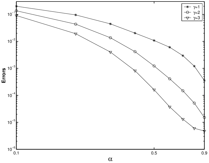
In Figure 2, we demonstrate the positive influence of time graded mesh power γ\gamma on the error that remains valid for different values of 0.1≤α≤0.90.1\leq\alpha\leq 0.9. The errors achieved as a function of α\alpha for different values of γ\gamma, but for a fixed N=60N=60 and a fixed m=2.m=2.

Refer to caption
Fig. 2: The errors ‖|Uh−u|‖10|||U_{h}-u|||_{10} for Example 1 plotted against α\alpha for different values of γ\gamma and fixed N=60N=60 with m=2m=2.

Next, we test the performance of the spatial finite elements discretizaton (order degree rr) of the scheme (4). A uniform spatial mesh that consists of NxN_{x} subintervals where each is of width hh will be used. The time step-size kk and the degree of the time-stepping DPG discretization are chosen such that the spatial error is dominating. Hence, from Theorem 3, a convergence of order O⁡(hr+1)O(h^{r+1}) is expected. We illustrated these results in Table 2 for r=1, 2, 3.r=1,\,2,\,3.

NxN_{x} r=1r=1 r=2r=2 r=3r=3
10 5.638e-03 1.576e-04 2.633e-06
20 1.426e-03 1.983 1.796e-05 3.133 1.568e-07 4.069
30 6.367e-04 1.988 4.730e-06 3.291 2.998e-08 4.081
40 3.584e-04 1.998 1.979e-06 3.029 9.172e-09 4.117
60 1.592e-04 2.002 6.240e-07 2.847
Table 2: The errors ‖|Uh−u|‖10|||U_{h}-u|||_{10} for Example 1 with α=0.5\alpha=0.5. We observe a spatial convergence of order hr+1h^{r+1} for r=1, 2, 3.r=1,\,2,\,3. The time mesh will be chosen such that the spatial errors are dominating.

5.2 Example 2

(Less smooth) We choose u0u_{0} and ff in problem (1) such u⁡(x,t)=t1−α​sin⁡(π​x)u(x,t)=t^{1-\alpha}{\sin}(\pi x) is the exact solution. It can be seen that the regularity conditions in (8)  hold for σ=1−α\sigma=1-\alpha and δ=2−α\delta=2-\alpha. Thus, it is less smooth than Example 1 in the time variable. As in the previous example, we demonstrate tabularly and graphically optimal convergence rates of the DPG-FE scheme (4) in the time direction on the non-uniformly graded meshes in (9). To do so, we take a relatively large number of subintervals in space and choose rr (the degree of the approximate finite element solution in the spatial variable) appropriately so that the temporal errors are dominating. Thus, by Theorem 3, convergence of order O⁡(k2​m+α)O(k^{2m+\alpha}) for γ≥2​m+1+α1−α\gamma\geq\frac{2m+1+\alpha}{1-\alpha} is anticipated. However, and as in Example 1, the numerical results in Table 3 illustrate more optimistic convergence rates. We observed a uniform global error bounded by C​kmin⁡{γ⁡(1−α),m+1}Ck^{\min\{\gamma(1-\alpha),m+1\}} for γ≥1\gamma\geq 1, which is optimal for γ≥(m+1)/(1−α)\gamma\geq(m+1)/(1-\alpha) (relaxed) and not for γ≥2​m+α+11−α\gamma\geq\frac{2m+\alpha+1}{1-\alpha} as the theory suggested. For graphical illustrations, see Figure 3.

NN γ=1\gamma=1 γ=2\gamma=2 γ=3\gamma=3 γ=3.6\gamma=3.6 γ=4.2\gamma=4.2
m=1m=1
20 9.3e-03 1.5e-03 1.5e-03
40 5.6e-03 0.73 4.5e-04 1.7 3.9e-04 2.0
80 3.5e-03 0.67 1.7e-04 1.4 9.9e-05 2.0
160 2.2e-03 0.68 6.5e-05 1.4 2.5e-05 2.0
320 1.4e-03 0.68 2.5e-05 1.4 5.7e-06 2.1
m=2m=2
10 6.3e-03 1.4e-03 3.2e-04 2.4e-04 3.7e-04
20 3.8e-03 0.71 5.2e-04 1.5 6.7e-05 2.3 3.3e-05 2.9 3.1e-05 3.6
30 2.9e-03 0.69 2.9e-04 1.4 2.8e-05 2.2 1.1e-05 2.6 7.5e-06 3.5
40 2.4e-03 0.69 1.9e-04 1.4 1.5e-05 2.2 5.5e-06 2.6 2.9e-06 3.3
50 2.0e-03 0.69 1.4e-04 1.4 9.2e-06 2.1 3.1e-06 2.6 1.5e-06 3.1
80 1.5e-03 0.69 7.2e-05 1.4 3.4e-06 2.1 9.2e-07 2.6
Table 3: The errors ‖|Uh−u|‖10|||U_{h}-u|||_{10} for different time mesh gradings with m=1m=1 and m=2m=2 (that is, piecewise linear and piecewise quadratic DPG time stepping solution), and α=0.3\alpha=0.3. We observe convergence of order k(1−α)​γ(=k0.7​γ)k^{(1-\alpha)\gamma}(=k^{0.7\gamma}) for 1≤γ≤(m+1)/(1−α)1\leq\gamma\leq(m+1)/(1-\alpha).
Refer to captionRefer to caption
Fig. 3: The errors ‖|Uh−u|‖10|||U_{h}-u|||_{10} for Example 2 plotted against NN for different choices of γ\gamma and for m=2, 3m=2,\,3, with α=0.3\alpha=0.3.

References

  • [1] C. L. Bottasso, S. Micheletti, and R. Sacco, The discontinuous Petrov–-Galerkin method for elliptic problems, Computer Methods Appl. Mech. Eng., 191 (2002), 3391–-3409.
  • [2] C. L. Bottasso, S. Micheletti, and R. Sacco, A multiscale formulation of the discontinuous Petrov–-Galerkin method for advective–diffusive problems, Computer methods Appl. Mech. Eng., 194 (2005) 2819–-2838.
  • [3] C-M. Chen, F. Liu, V. Anh, and I. Turner, Numerical methods for solving a two–dimensional variable-order anomalous subdiffusion equation, Math. Comp., 81, (2012) 345–366.
  • [4] E. Cuesta and C. Lubich, C. Palencia, Convolution quadrature time discretization of fractional diffusive-wave equations, Math. Comp., 75, (2006) 673–696.
  • [5] M. Cui, Compact finite difference method for the fractional diffusion equation, J. Comput. Phys., 228, (2009) 7792–7804.
  • [6] M. Cui, Convergence analysis of high-order compact alternating direction implicit schemes for the two-dimensional time fractional diffusion equation, Numer. Algor., 62, (2013) 383–409.
  • [7] L. Demkowicz and J. Gopalakrishnan, A class of discontinuous Petrov–-Galerkin methods. part I: The transport equation, Computer Methods Appl. Mech. Eng., 199 (2010), 1558-–1572.
  • [8] G.G. Gao and Z.Z. Sun, A box-type scheme for fractional sub-diffusion equation with Neumann boundary conditions, J. Comput. Phys., 230, (2011) 6061-–6074.
  • [9] B. L. Hulme, One-step piecewise polynomial Galerkin methods for initial value problems, Math. Comp., 26, (1972) 881–891.
  • [10] B. Jin, R. Lazarov, and Z. Zhou, Error estimates for a semidiscrete finite element method for fractional order parabolic equations, SIAM J. Numer. Anal., 51, (2013) 445–466.
  • [11] B. Jin, R. Lazarov, and Z. Zhou, On two schemes for fractional diffusion and diffusion-wave equaiton, http://arxiv.org/pdf/1404.3800v1.pdf, (2014).
  • [12] T. A. M. Langlands and B. I. Henry, The accuracy and stability of an implicit solution method for the fractional diffusion equation, J. Comput. Phys., 205, (2005) 719–936.
  • [13] X. Li and C. Xu, A space-time spectral method for the time fractional diffusion equation, SIAM J. Numer. Anal., 47, (2009), 2108–2131.
  • [14] T. Lin, Y. Lin, M. Rao and S. Zhang, Petrov-Galerkin methods for linear Volterra integro-differential equations, SIAM J. Numer. Anal., 38, (2000) 937–963.
  • [15] Y. Lin and C. Xu, Finite differnce/spectral approximations for the time-fractional diffusion equation, J. Comput. Phys., 225, (2007), 1533–1552.
  • [16] F. Liu, C. Yang and K. Burrage, Numerical method and analytical technique of the modified anomalous subdiffusion equation with a nonlinear source term, Comput. Appl. Math., 231, (2009) 160–176.
  • [17] A.M. Mathai, R. K, Saxena and H. J. Haubold, The H-Function: Theory and Applications, Springer, 2011
  • [18] W. McLean, Regularity of solutions to a time-fractional diffusion equation, ANZIAM J., 52, (2010) 123–138.
  • [19] W. McLean and K. Mustapha, A second-order accurate numerical method for a fractional wave equation, Numer. Math., 105, (2007) 481–510.
  • [20] W. McLean and K. Mustapha, Convergence analysis of a discontinuous Galerkin method for a sub-diffusion equation, Numer. Algor., 52, (2009) 69–88.
  • [21] K. Mustapha, A Petrov-Galerkin method for integro-differential equations with a memory term, ANZIAM J., 50, (2008) 610–624.
  • [22] K. Mustapha, An implicit finite difference time-stepping method for a sub-diffusion equation, with spatial discretization by finite elements, IMA J. Numer. Anal., 31, (2011) 719–739.
  • [23] K. Mustapha and J. AlMutawa, A finite difference method for an anomalous sub-diffusion equation, theory and applications, Numer. Algor., (2012).
  • [24] K. Mustapha and W. McLean, Uniform convergence for a discontinuous Galerkin, time stepping method applied to a fractional diffusion equation, IMA J. Numer. Anal., 32, (2012) 906–925.
  • [25] K. Mustapha and W. McLean, Superconvergence of a discontinuous Galerkin method for fractional diffusion and wave equations, SIAM J. Numer. Anal., 51, (2013) 491–515
  • [26] K. Mustapha and D. Schoetzau, Well-posedness of h​p−hp-version discontinuous Galerkin methods for fractional diffusion wave equations, IMA J. Numer. Anal., (2013), accepted
  • [27] I. Podlubny, Fractional Differential Equations, Academic Press, San Diego, 1999.
  • [28] J. Quintana-Murillo and S.B. Yuste, An explicit difference method for solving fractional diffusion and diffusion-wave equations in the Caputo form, J. Comput. Nonlin. Dyn., 6, (2011) 021014.
  • [29] C. Schwab, pp and h​php-Finite Element Methods – Theory and Applications in Solid and Fluid Mechanics, Oxford University Press, 1998.
  • [30] P. Smith, I. Morrison, K. Wilson, N. Fernandez, and R. Cherry, Anomalous diffusion of major histocompatability complex class I molecules on HeLa cells determined by single particle tracking, Bio. Phys. J., 76, (1999) 3331–3344.
  • [31] N. H. Sweilam, M. M. Khader and A. M. S. Mahdy, Crank-Nicolson finite difference method for solving time-fractional diffusion equation, J. Fract. Cal. Appl., 2 (2012) 1–9.
  • [32] V. E. Tarasov, Fractional Dynamics: Applications of Fractional Calculus to Dynamics of Particles, Fields and Media (Nonlinear Physical Science), Springer, 2011
  • [33] H. Wanga and K. Wanga, An O⁡(N​l​o​g2​N)O(N\,log^{2}N) alternating-direction finite difference method for two-dimensional fractional diffusion equations, J. Comput. Phys., 230, (2011) 7830–7839.
  • [34] S. B. Yuste and L. Acedo, An explicit finite difference method and a new von Neumann-type stability analysis for fractional diffusion equations, SIAM J. Numer. Anal., 42, (2005) 1862–1874.
  • [35] S.B. Yuste, J. Quintana-Murillo, On Three Explicit Difference Schemes for Fractional Diffusion and Diffusion-Wave Equations, Phys. Scripta T136, (2009) 014025.
  • [36] F. Zengo, C. LI, F. Liu, I. Turner, The use of finite difference/element approaches for solving the time-fractional subdiffusion equation, SIAM J. Sci. Comput., 35, (2013) A2976–A3000.
  • [37] Ya-nan Zhang, Zhi-zhong Sun, Alternating direction implicit schemes for the two-dimensional fractional sub-diffusion equation, J. Comput. Phys., 230, (2011) 8713–8728.
  • [38] X. Zhao and Z-z. Sun, A box-type scheme for fractional sub-diffusion equation with Neumann boundary conditions, J. Comput. Phys., 230, (2011) 6061–6074.
  • [39] P. Zhuang, F. Liu, V. Anh, and I. Turner, New solution and analytical techniques of the implicit numerical methods for the anomalous sub-diffusion equation, SIAM J. Numer. Anal., 46, (2008) 1079–1095.