Quark confinement: dual superconductor picture based on a non-Abelian Stokes theorem and reformulations of Yang-Mills theory
Abstract
The purpose of this paper is to review the recent progress in understanding quark confinement. The emphasis of this review is placed on how to obtain a manifestly gauge-independent picture for quark confinement supporting the dual superconductivity in the Yang-Mills theory, which should be compared with the Abelian projection proposed by ’t Hooft. The basic tools are novel reformulations of the Yang-Mills theory based on change of variables extending the decomposition of the Yang-Mills field due to Cho, Duan-Ge and Faddeev-Niemi, together with the combined use of extended versions of the Diakonov-Petrov version of the non-Abelian Stokes theorem for the Wilson loop operator.
Moreover, we give the lattice gauge theoretical versions of the reformulation of the Yang-Mills theory which enables us to perform the numerical simulations on the lattice. In fact, we present some numerical evidences for supporting the dual superconductivity for quark confinement. The numerical simulations include the derivation of the linear potential for static interquark potential, i.e., non-vanishing string tension, in which the “Abelian” dominance and magnetic monopole dominance are established, confirmation of the dual Meissner effect by measuring the chromoelectric flux tube between quark-antiquark pair, the induced magnetic-monopole current, and the type of dual superconductivity, etc. In addition, we give a direct connection between the topological configuration of the Yang-Mills field such as instantons/merons and the magnetic monopole.
We show especially that magnetic monopoles in the Yang-Mills theory can be constructed in a manifestly gauge-invariant way starting from the gauge-invariant Wilson loop operator and thereby the contribution from the magnetic monopoles can be extracted from the Wilson loop in a gauge-invariant way through the non-Abelian Stokes theorem for the Wilson loop operator, which is a prerequisite for exhibiting magnetic monopole dominance for quark confinement. The Wilson loop average is calculated according to the new reformulation written in terms of new field variables obtained from the original Yang-Mills field based on change of variables. The Maximally Abelian gauge in the original Yang-Mills theory is also reproduced by taking a specific gauge fixing in the reformulated Yang-Mills theory. This observation justifies the preceding results obtained in the maximal Abelian gauge at least for gauge-invariant quantities for gauge group, which eliminates the criticism of gauge artifact raised for the Abelian projection. The claim has been confirmed based on the numerical simulations.
However, for (), such a gauge-invariant reformulation is not unique, although the extension along the line proposed by Cho, Faddeev and Niemi is possible. In fact, we have found that there are a number of possible options of the reformulations, which are discriminated by the maximal stability group of , while there is a unique option of for . The maximal stability group depends on the representation of the gauge group, to that the quark source belongs. For the fundamental quark for , the maximal stability group is , which is different from the maximal torus group suggested from the Abelian projection. Therefore, the chromomagnetic monopole inherent in the Wilson loop operator responsible for confinement of quarks in the fundamental representation for is the non-Abelian magnetic monopole, which is distinct from the Abelian magnetic monopole for the case. Therefore, we claim that the mechanism for quark confinement for () is the non-Abelian dual superconductivity caused by condensation of non-Abelian magnetic monopoles. We give some theoretical considerations and numerical results supporting this picture. Finally, we discuss some issues to be investigated in future studies.
Keywords:
quark confinement , magnetic monopole , Wilson loop , dual superconductivity , Abelian projection , Maximally Abelian gauge , non-Abelian Stokes theoremPACS
12.38.Aw , 14.70.Dj , 12.38.Bx , 12.38.LgPreprint: CHIBA-EP-209 v3
KEK Preprint 2014-23
1 Introduction
It is widely accepted that quantum chromodynamics (QCD) is the most fundamental quantum field theory for describing the strong interactions mediated by gluons whose dynamics is governed by the Yang-Mills theory [1]. In experiments, however, the fundamental degrees of freedom for QCD, i.e., quarks and gluons, have never been observed in the isolated form. Only the color singlet combinations known as hadrons (mesons and baryons) and candidates of glueballs are observed. This experimental fact can be explained from a hypothesis of color confinement: Colored objects cannot be observed and only color singlet objects (colorless composites) can be observed in Nature. Indeed, quarks and gluons have their own color charges and hence they cannot be observed according to this hypothesis. From this viewpoint, quark confinement is a special case of color confinement and seems to be more tractable than color confinement. For quark confinement, indeed, we have a well-known gauge-invariant criterion due to Wilson [2], i.e., area law of the Wilson loop average, which is equivalent to the linear potential for the static quark-antiquark potential. Whereas the gauge-invariant criterion for color confinement is still unknown to the best of the author knowledge.
We wish to clarify the basic mechanism for quark confinement, which enables us to explain how and why quark confinement occurs in Nature. A promising scenario for quark confinement called the dual superconductivity picture has been proposed in 1970s by Nambu, ’t Hooft, Mandelstam [3]. The dual superconductivity is supposed to be realized as the electric–magnetic duality of the ordinary superconductivity: The dual superconductivity could be realized as a consequence of condensation of magnetic monopoles, i.e., magnetically charged objects, just as the ordinary superconductivity is caused by condensation of the Cooper pairs, i.e., electrically charged objects. In the vacuum of dual superconductor, the dual Meissner effect squeezes the chromoelectric flux between a quark and an antiquark into a tube like region to form the hadronic string. The key ingredients of the dual superconductor picture for the Yang-Mills theory vacuum are the existence of chromomagnetic monopole condensation and the dual Meissner effect. In order to establish the dual superconductivity, therefore, it is a first step to show the existence of magnetic monopole in QCD, i.e., chromomagnetic monopole, which is to be condensed in the Yang-Mills theory [1], since chromomagnetic monopole is an indispensable ingredient for dual superconductivity in QCD.
At present, there is no analytical proof of the existence of the condensate of the magnetic monopole in gluodynamics and in QCD. However, in all theories allowing for an analytical proof of confinement, confinement is due to the condensation of magnetic monopoles. 4D compact electrodynamics (compact lattice gauge theory) [4], 3D Georgi-Glashow model [5] and a supersymmetric Yang-Mills theory [6].
In view of this, we recall well-known examples of magnetic monopoles appeared so far in gauge field theories. In the Maxwell electromagnetism, the Dirac magnetic monopole [7, 8] is realized by introducing singularities in the gauge potential. Otherwise, the Bianchi identity leads to identically vanishing magnetic current. In the non-Abelian gauge theory with (adjoint) matter fields such as the Georgi-Glashow model, one can construct the ’t Hooft-Polyakov magnetic monopole [9] without introducing the singularity in the Yang-Mills field thanks to the extra degrees of freedom coming from the matter fields. See e.g. [10, 11] for reviews.
- 1.
The Dirac magnetic monopole [7] in the Maxwell theory is realized when and only when there are singularities in the gauge potential , leading to the violation of the Bianchi identity for gauge field strength . As far as the gauge potential is non-singular, indeed, the magnetic-monopole current vanishes identically:11 1 Here and are 1-forms and is a 2-form. And is the exterior derivative, is the codifferential and ∗ is the Hodge duality operation. The exterior derivative has the nilpotency .
(1.1) - 2.
The ’t Hooft-Polyakov magnetic monopole [9] in the presence of the Higgs fields (in the adjoint representation) is obtained due to the spontaneous symmetry breaking of the original gauge symmetry to a subgroup :
(1.2)
Then we can raise a basic question: What kind of magnetic monopoles can be defined in QCD and Yang-Mills theory without the scalar fields? Currently, there are at least two methods available to define the chromomagnetic monopole in the Yang-Mills theory, i.e., magnetic monopole in the non-Abelian gauge theory in the absence of matter fields:
- 1.
Abelian projection [13]
Abelian magnetic monopole is obtained due to explicit breaking (partial gauge fixing) of the original gauge group to the maximal torus subgroup with being the rank of the gauge group : , e.g., , . The magnetic monopole is identified with the gauge-fixing defect.
- 2.
Field decomposition [14, 15, 16, 17],[21, 22, 23] and change of variables [18, 19, 20],[24, 25, 26, 27, 28, 29, 30, 31, 32, 33]
It is possible to realize magnetic monopoles in the pure non-Abelian gauge theory in the absence of the adjoint Higgs field, without explicitly introducing singularities in the gauge connection and without breaking the original gauge symmetry and color symmetry. This is done by performing a gauge-covariant decomposition of the gluon field by introducing the local color direction field.
The first method, i.e., Abelian projection proposed by ’t Hooft [13] is well known and has been conventionally and extensively used to extract magnetic monopoles from the Yang-Mills field. For instance, the Abelian projection for is regarded as a partial gauge fixing from the original gauge group to the maximal torus subgroup :
| (1.3) |
This is an explicit breaking of the (local) gauge symmetry.22 2 The conventional Abelian gauge breaks the original local symmetry to leave the local and the global unbroken, but breaks the global . The new reformulation based on the second method leaves the local and the global unbroken (color rotation invariant).
Within the Abelian projection, the relevant data supporting the validity of the dual superconductor picture have been accumulated by numerical simulations on the lattice especially since 1990 and some of the theoretical predications have been confirmed by these investigations. In the maximally Abelian gauge (MA gauge, MAG) [34] for , as a realization of the Abelian projection, especially, the infrared Abelian dominance [13, 35] was confirmed by numerical simulations on the lattice [36, 39, 40], and subsequently magnetic monopole dominance [37, 38] was also confirmed in the string tension in the linear potential for the static quark-antiquark potential. The infrared Abelian dominance was also confirmed for the gluon propagator by exhibiting the rapid fall-off of the off-diagonal gluon propagator, leading to the non-vanishing off-diagonal gluon mass. For the Yang-Mills theory, thus, the following characteristic features supporting the dual superconductivity for confinement were established in the MA gauge for :
- 1.
- 2.
- 3.
However, they are confirmed only in specific gauges, i.e., Abelian gauges, such as the MA gauge, Laplacian Abelian gauge [42, 43] and maximal center gauge [48]. All these gauge fixing break color symmetry explicitly. See, e.g., [44, 45, 46, 47] for reviews of Abelian projection and Abelian gauge and also [48, 49, 50] for more topics. See e.g., [51] for dual superconductor models.
The second method less familiar than the first one is based on the gauge-covariant decomposition of the Yang-Mills field, which has been proposed independently by Cho [15, 21] and Duan and Ge [14] at nearly the same time as the ’t Hooft proposal of the Abelian projection, and later readdressed by Faddeev and Niemi [16, 22] and Shabanov [17]. Therefore, it is called the Cho–Duan-Ge (CDG) decomposition or Cho–Duan-Ge–Faddeev-Niemi (CDGFN) decomposition, or Cho–Duan-Ge–Faddeev-Niemi–Shabanov (CDGFNS) decomposition. By using the second method, the magnetic monopole in the Yang-Mills theory is constructed in a gauge-independent way. The first method, i.e., Abelian projection is reproduced as a special limit of the second method, i.e., Field decomposition. In other words, the first method can be regarded as a gauge-fixed version of the second method. The second method including the extension to explained later has been furthermore developed especially in the last decade by the Chiba University group [18, 19, 20, 24] and Chiba/KEK/Fukui (Takamatsu) collaborations [25, 26, 27, 28, 29, 30, 31, 32, 33].
The key ingredient of the decomposition is the introduction of a novel field which represents the (local) Abelian direction embedded in the non-Abelian gauge degrees of freedom at each space–time point. The decomposition begins with the introduction of the unit field , which we call the color direction field or color field for short. For , the color field has three components and a unit length. Therefore, it has two independent degrees of freedom. In the Lie-algebra notation , the color field is expressed as
| (1.4) |
where () denotes the Pauli matrices. The constraint of the unit length is represented as . For , therefore, the color field takes the value in the Lie algebra of , which is easily observed using the adjoint orbit representation without loss of generality:
| (1.5) |
According to the decomposition, the Yang-Mills gauge field can be separated into the restricted field (corresponding to the “Abelian” part in the Abelian projection) and the remaining field :
| (1.6) |
in such a way that
- 1.
[gauge-independent “Abelian” projection] The restricted part is the dominant mode responsible for quark confinement. The non-Abelian Wilson loop operator defined in terms of the original field is entirely rewritten in terms of the restricted field alone, i.e.,
(1.7) Furthermore, it is rewritten into the surface integral of the invariant field strength of the Abelian type over the surface bounded by the loop :
(1.8) where is defined from the color direction field and the field strength of the restricted field .
(1.9) This fact follows from the non-Abelian Stokes theorem for the Wilson loop operator. (The restricted field corresponds to the Abelian part in the Abelian projection.)
- 2.
[infrared restricted field (“Abelian”) dominance] The remaining part decouples in the low-energy regime. The correlation function of the field exhibits the rapid fall-off of the exponential type. This suggests that the field acquires the gauge-invariant mass dynamically. This leads to the infrared restricted field (“Abelian”) dominance. The dynamical mass can originate from the gauge-invariant vacuum condensate of mass dimension-two . Note that is a gauge-invariant operator of mass dimension two, which corresponds to the BRST invariant operator of mass dimension two, constructed from the gluon and ghost [52]. The existence of dimension-two condensate has been examined by an analytical method [20] and numerical one [25].
The restricted part (“Abelian” part) responsible for quark confinement can be extracted from the non-Abelian gauge field in the gauge-independent way without breaking color symmetry. Using the restricted field alone, we can give a definition of a gauge-invariant magnetic monopole current :
| (1.10) |
giving the magnetic charge subject to the Dirac quantization condition (which is confirmed by analytical and numerical methods [27]) and magnetic monopole dominance in the string tension (confirmed by numerical method [27, 29]).
The second method is more involved than the first one, but it is now recognized to be superior in some aspects to the first one:
- 1.
The gauge-invariance of the chromomagnetic monopole is guaranteed from the beginning by construction.
- 2.
The direct relevance of the chromomagnetic monopole to the Wilson loop and “Abelian” dominance in the operator level are manifest via a non-Abelian Stokes theorem for the Wilson loop operator.
The CDG decomposition of the Yang-Mills field variable is translated to the change of variables. Then the Yang-Mills theory was reformulated in terms of new variables based on a new viewpoint of the CDG decomposition proposed in [18, 19]. The path integral quantization has been completed by giving the action and the integration measure in the closed form in terms of new field variables.
The second method enables us to answer the following questions which are unclear in the first one.
- 1.
- 2.
How to define the magnetic monopole to be condensed in Yang-Mills theory in the gauge-independent way even in absence of any scalar field, in sharp contrast to the Georgi-Glashow model in which scalar field in the adjoint representation plays the important role in constructing the ’t Hooft-Polyakov magnetic monopole.
The purpose of this paper is to give a review of recent developments for understanding quark confinement by paying special attention to the second method in comparison with the first one, which will give more insight into the mechanism for quark confinement. In particular, we emphasize some aspects of the second method superior to the first one for establishing the dual superconductivity in Yang-Mills theory. In particular, the reformulation enables us to extract in a gauge-independent manner the dominant degrees of freedom that are relevant to quark confinement in the sense of the Wilson criterion in such a way that they reproduce the original string tension in the linear part of the static quark-antiquark potential.
Moreover, we have given a new reformulation for the lattice Yang-Mills theory, so that it reproduces the continuum Yang-Mills theory in the naive continuum limit. This new reformulation of the Yang-Mills field theory on a lattice enables us to perform numerical simulations on a lattice. In fact, we present the results of numerical simulations obtained based on this framework and give some numerical evidences supporting the dual superconductivity for quark confinement. For the Yang-Mills theory, the second method has already reproduced all characteristic features supporting the dual superconductivity for confinement obtained so far by the first method:
- 1.
infrared restricted field (or “Abelian”) dominance in the string tension (calculated from the Wilson loop average) [29]: This is called the “Abelian” dominance or restricted field dominance to distinguish it from the Abelian dominance obtained under the gauge-dependent Abelian projection.
- 2.
magnetic monopole dominance in the string tension (calculated from the Wilson loop average) [27]:
- 3.
restricted field propagator dominance, or rapid fall-off of the remaining field propagator with a non-vanishing mass [28]:
- 4.
confirmation of the dual Meissner effect by measuring the chromoelectric flux tube between quark-antiquark pair, the induced magnetic-monopole current around the chromoelectric flux tube, and the type of dual superconductivity, etc. [29]:
In addition, we give a direct connection between the magnetic monopole and the other topological configurations of the Yang-Mills field such as instantons/merons.
For the Yang-Mills theory, the gauge-independent results obtained in the second method guarantee the validity of those obtained by the preceding studies based on the first method, since the MA gauge is reproduced as a special gauge choice of the gauge-independent second method. This fact removes the criticism raised for the results obtained in the MA gauge for . This is a great progress toward the goal of understanding the mechanism of quark confinement. But, it turns out that the cases of and () are not necessarily the straightforward extensions of the .
Subsequently, we proceed to consider the general Yang-Mills theory () including a realistic case of three colors . Even in the Yang-Mills theory, we can extract magnetic monopoles using the Abelian projection, which breaks explicitly the original gauge group into the maximal torus subgroup :
| (1.11) |
Then, the Abelian projection yields kinds of Abelian magnetic monopoles with different magnetic charges, in agreement with the observation due to the non-trivial homotopy group:
| (1.12) |
Therefore, it tends to assume that magnetic monopoles of kinds are necessary to realize quark confinement in the Yang-Mills theory from the viewpoint of the dual superconductivity, while a single magnetic monopole is sufficient in the Yang-Mills theory. However, it is not yet established whether or not kinds of magnetic monopoles are necessary or indispensable to achieve quark confinement in Yang-Mills theory ().
Keeping this question in mind, we proceed to extend the new formulation of Yang-Mills theory to the case. For the Yang-Mills field, the decomposition as an extension of the CDGFN decomposition was proposed by Cho [21, 23] and Fadeev-Niemi [22] which we call the Cho–Faddeev-Niemi (CFN) decomposition. They introduced color direction fields and decomposed the Yang-Mills field by way of the color fields in the similar way to the case. This is reasonable, since the group has Abelian directions specified by the Cartan subalgebra whose generators mutually commute, i.e., (). Then the color field takes the value in the Lie algebra of , which is represented by
| (1.13) |
Consequently, the Yang-Mills theory is rewritten in terms of new variables constructed through the color fields just defined, just as done in the case. This decomposition and subsequent reformulation enables us to give a gauge-independent Abelian-projection. The CFN scenario lead to the kinds of gauge-invariant magnetic monopoles. However, whether or not this reformulation gives the best description for quark confinement is another problem to be examined. This is because the reformulation which is equivalent to the original Yang-Mills theory is not unique. Which reformulation gives the best description for confinement should be determined by imposing further requirements.
Rather, we claim that even in the Yang-Mills theory a single magnetic monopole is sufficient to achieve confinement, when quarks belong to the fundamental representation of the color gauge group. In fact, this scenario was originally proposed in [59, 60, 61] based on a consideration from a non-Abelian Stokes theorem for the Wilson loop operator [55, 56, 57, 58], which is more elaborated in [62, 63, 64, 65] (See [66, 67, 68, 69, 70, 71, 72] for other versions of non-Abelian Stokes theorem). In order to consider confinement of quarks in the specified representation based on the Wilson loop operator, we adopt the color field taking the value in the Lie algebra of ,
| (1.14) |
where is a subgroup of called the maximal stability subgroup which is determined once the highest-weight state of a given representation is chosen. This is the best theoretical choice deduced from the non-Abelian Stokes theorem for the Wilson loop operator. For the fundamental representation of , we find that the maximal stability group is due to the non-Abelian Stokes theorem for the Wilson loop operator. The fact that the target space of the color field is the coset suggests a single magnetic monopole inherent in the Wilson loop operator is responsible for confining quarks in the fundamental representation, in agreement with the non-trivial Homotopy group:
| (1.15) |
which is independent of , in sharp contrast to the Abelian projection (1.12).
By adopting a single color field alone, we can reformulate the Yang-Mills theory in terms of new variables. This fact elucidates the crucial difference between the decomposition in the preceding approach and the change of variables in our approach, which we emphasize in this paper. In fact, this observation can be substantiated by making use of a novel reformulation of Yang-Mills theory using new variables completed in [24] combined with the non-Abelian Stokes theorem for the Wilson loop operator [62]. The new formulation is an extension of the CFN proposals, since the CFN case is obtained as a special option of the new formulation. The reformulation can exhaust all the options discriminated by the possible choice of the maximal stability groups. Among them, the reformulation with a single color field is called the minimal option, while the conventional CFN option is called the maximal option.
For , in particular, there are only two possibilities: maximal option and minimal option. The minimal option with the maximal stability subgroup:
| (1.16) |
is a new option (overlooked so far) suited for representing the Wilson loop in the fundamental representation, on which we focus in this review, while the maximal one with the maximal torus subgroup as a maximal stability group:
| (1.17) |
enables us to give a gauge-independent reformulation of the Abelian projection represented by the conventional MA gauge. The maximal option is equivalent to the CFN case. For (), there are more options other than the maximal and minimal ones. For instance, see [24] for concrete examples of case. In this review we consider only maximal and minimal options and we do not discuss other options.
For in the minimal option, the resulting chromomagnetic monopole is not the Abelian magnetic monopole, rather a non-Abelian magnetic monopole with non-trivial internal structure , of which only the degree of freedom is seen by a single magnetic charge in the long distance. Therefore, we propose the non-Abelian dual superconductivity as a mechanism for confining quarks in the fundamental representation in the Yang-Mills theory.
In the static potential for a pair of quark and antiquark in the fundamental representation, it has been demonstrated: (i) the infrared restricted-field dominance (or “Abelian” dominance) (which is a gauge-independent (invariant) extension of the conventionally called infrared Abelian dominance): the string tension obtained from the restricted field reproduces the string tension of the original YM field, , (ii) the gauge-independent non-Abelian magnetic monopole dominance: the string tension extracted from the restricted field is reproduced by only the (non-Abelian) magnetic monopole part , . We have also confirmed the dual Meissner effect by measuring the chromoelectric flux tube between quark-antiquark pair, the induced magnetic-monopole current around the chromoelectric flux tube, and the type of dual superconductivity, etc. the Yang-Mills theory in the minimal option. These results are based on the lattice reformulation of Yang-Mills theory constructed in [30, 31] and the results of numerical simulations on the lattice performed in [32, 33].
Finally, it is fair to mention that other mechanisms were proposed and investigated. In the vortex (condensation) picture, the the vacuum of the Yang-Mills theory is presumed to be dominated by long vortices carrying multiples of magnetic flux [73, 74, 75, 76]. In particular, another very popular one was the proposal based on center vortices [77] as topological excitations that disorder the Wilson loop. The community was somewhat divided and arguing about one picture or the other, without reaching a consensus, until slowly people moved on to study other aspects of confinement. This paper does not discuss the center vortex picture for confinement. See e.g., [48] for the review on maximal center gauge and also [78, 79, 80] for the relationship between the center vortex and magnetic monopole.
This paper is organized as follows.
In section 2, we give a short review on the original idea of the Abelian projection as a partial gauge fixing to demonstrate how magnetic monopoles are obtained in the Yang-Mills theory in the absence of the scalar field. We give the basic knowledge on the MA gauge as a realization of the Abelian projection, and briefly summarize the remarkable results obtained in the MA gauge by the numerical simulations on the lattice in the last century.
In section 3, we give a review on the CDG decomposition of the Yang-Mills field, which is another method to define magnetic monopoles in the Yang-Mills theory in the absence of the scalar field. The decomposition is uniquely determined by solving the defining equations. We explain the relationship between the CDG decomposition and the Abelian projection.
In section 4, we give a reformulation of the Yang-Mills theory rewritten in terms of new variables. The new variables are obtained from the original Yang-Mills field based on a (non-linear) change of variables. The reformulated Yang-Mills theory is constructed based on the new viewpoint proposed by Kondo, Murakami and Shinohara [19, 18], which resolves some questions raised for the original idea of the CDG decomposition and gives a clear guidance for further developments. Indeed, it guarantees that the reformulated Yang-Mills theory written in terms of new variables is equipollent to the original Yang-Mills theory. This gives a definite prescription of defining the quantum Yang-Mills theory according to the path-integral quantization so that the action integral and the integration measure are explicitly written in the closed form in terms of new variables.
In section 5, we show how the reformulation given for the Yang-Mills theory using new variables can be extended to the Yang-Mills theory (). For the gauge group with rank , it possible to introduce color fields which will play the role of keeping the color symmetry (or recovering the color symmetry lost by adopting the Abelian projection) and defining a gauge-invariant magnetic monopole in case, which is the choice of Cho and Faddeev-Niemi. However, it is shown [24] that this procedure is not necessarily a unique starting point to reformulate the Yang-Mills theory and that only a single color field is sufficient to reformulate the Yang-Mills theory irrespective of the number of color . Moreover, we find that the minimal case is indispensable in order to understand confinement of quarks in the fundamental representation, which will be shown in the next section based on the non-Abelian Stokes theorem for the Wilson loop operator.
In section 6, we give a (Diakonov-Petrov) version of non-Abelian Stokes theorem for the Wilson loop operator. The presentation [58, 59, 60, 62] based on the coherent state of the Lie group and the path-integral representation is more systematic or universal than the original derivation by Diakonov and Petrov [55]. This form is quite useful to discuss quark confinement combined with the reformulation. In fact, it turns out that the Wilson loop is a probe of the gauge-invariant magnetic monopole defined in this reformulation. We can define the gauge-invariant magnetic monopole from the Wilson loop operator which is gauge invariant by definition. The magnetic monopole is inherent in the Wilson loop operator. The non-Abelian Stokes theorem tells us why the restricted field dominance follows from the Wilson loop operator.
In section 7, we identify the restricted field with the infrared dominant mode, and the remaining field with the high-energy relevant mode (infrared decoupled mode) in the original Yang-Mills field. This is based on a very interesting interrelationship between the field decomposition and the non-Abelian Stokes theorem. We try to obtain a low-energy effective theory written in terms of the restricted field alone, by integrating out the remaining field in the Yang-Mills action. For this purpose, we discuss how to extract the independent field degrees of freedom. To demonstrate the validity of the identification and the resulting low-energy effective theory, we discuss the crossover between the confinement/deconfinement and chiral-symmetry-breaking/restoration phase transitions in two color QCD at finite temperature. This is regarded as the first-principle derivation of the Polyakov-loop extended Nambu-Jona-Lasinio (PNJL) model which has been extensively used to study the QCD phase diagram.
In section 8, we show in an analytical and numerical ways (without using the numerical simulations) that the color direction field can be determined by solving the differential equation for the reduction condition for a given Yang-Mills field, since the color field plays the key role in the new reformulation of the Yang-Mills theory written in terms of the new variables. Moreover, we examine when circular loops of magnetic monopole exist in the four-dimensional Euclidean Yang-Mills theory, since they are expected to be responsible for quark confinement in the dual superconductor picture. As the given Yang-Mills fields, we examine some known solutions of the classical Yang-Mills field equation with non-trivial topology, i.e., one-meron, two-merons, one-instanton, and two-instantons.
In section 9, we give new lattice formulations which reduce in the continuum limit to the reformulation given in the continuum form. They enable us to study non-perturbative aspects by performing numerical simulations on the lattice. In fact, we give some numerical evidences for dual superconductivity in the Yang-Mills theory for and as enumerated in the above.
In section 10, we refer to some applications of the reformulations to other physical problems.
The final section is devoted to conclusion and discussion. Several Appendices are added to give technical details which are removed from the text.
1.1 Notations
In this review, we use the notation
| (1.18) |
in the sense that is defined by . On the other hand,
| (1.19) |
implies that is identically equal to . Moreover,
| (1.20) |
implies that follows from or that leads to ( follows from or that leads to ), and
| (1.21) |
implies that is equivalent to .
We use the following two different notations to express field variables.
The vector form:
| (1.22) |
or especially in the lattice gauge theory introduced later
| (1.23) |
or
| (1.24) |
where denotes the dimension of a gauge group , i.e., , e.g., for .
The Lie algebra form:
| (1.25) |
where denote the generators of the Lie algebra for the Lie group , e.g., for .
The two notations give the equivalent description. It should be understood that denotes the generator in the fundamental representation, unless otherwise stated.
We adopt the following normalization for the generators of the Lie algebra:
| (1.26) |
In order to lower and raise the indices , we need to introduce the Cartan metric and its inverse for the group . However, for group, this distinction can be avoided.33 3 This fact is explained in section 6. Therefore, we do not distinguish the lower and upper indices in this paper.
For , we can define three types of products: , and in the vector form by
| (1.27a) | ||||
| (1.27b) | ||||
| (1.27c) | ||||
which correspond to three operations in the Lie algebra form: , and as
| (1.28a) | ||||
| (1.28b) | ||||
| (1.28c) | ||||
Here we define the structure constants of the Lie algebra by
| (1.29) |
from the commutators among the generators:
| (1.30) |
while we use the anticommutator of the generators:
| (1.31) |
to define completely symmetric symbols:
| (1.32) |
The product of two Lie algebra valued functions, and , is rewritten as the sum of three types of products:
| (1.33) |
In other words, the Lie algebra is closed under the three products: and .
In what follows we use the same notation for two Lie-algebra valued functions and as that for the inner product in the vector notation in the sense that
| (1.34) |
and especially
| (1.35) |
We use for the inner product defined by
| (1.36) |
The Lie algebra of the group is sometimes denoted by
| (1.37) |
The degrees of freedom (d.o.f.) in the expression is denoted by
| (1.38) |
2 Abelian projection and Maximally Abelian gauge
2.1 Abelian projection and magnetic monopole
First of all, we review the idea of Abelian projection due to ’t Hooft [13], a method which enables us to extract magnetic monopole degrees of freedom from the Yang-Mills theory without the Higgs fields (i.e., scalar fields).
We consider the Yang-Mills theory with the gauge group on the -dimensional space–time . We denote by the Lie algebra of the group .
-
(1)
Let be a gauge-dependent (i.e., gauge non-invariant) local operator as a functional of the Yang-Mills field , which takes the value in the Lie algebra of the gauge group . Suppose that transforms according to the adjoint representation under the gauge transformation (gauge rotation):
(2.1) if the Yang-Mills field transforms
(2.2) - (2)
For the Hermitian operator , i.e., , we choose the local unitary transformation so that is diagonalized:
(2.3) where () are eigenvalues of .
After the Abelian projection, the original gauge group is explicitly broken to a subgroup :
| (2.4) |
where is the so-called the maximal torus subgroup or Cartan subgroup of , and the Weyl group is a discrete subgroup of which corresponds to the degrees of freedom for changing the ordering of the eigenvalues.44 4 See K and the textbook of the group theory, e.g., [81]. If the eigenvalues are ordered such that , the Weyl group is broken and only the maximal torus subgroup is left intact after the Abelian projection.
Therefore, the Abelian projection is regarded as a partial gauge fixing, since is a gauge-dependent quantity. This is indeed the gauge fixing because we cannot perform the original gauge transformation any more in order to keep the diagonal form of . Here the partial comes from the fact that there are exceptional parts as shown shortly. Consequently, the whole space–time points are classified into two categories:
- (a)
At the “non-degenerate” space–time point with the non-degenerate eigenvalues , i.e., all the eigenvalues at are different, the original gauge degrees of freedom are not completely fixed because any diagonal gauge rotation matrix:
(2.5) leaves invariant, i.e., or . Here is an element of the maximal Abelian subgroup . Therefore, the Abelian subgroup remains intact at the non-degenerate space–time point even after the Abelian projection.
- (b)
At the “degenerate” space–time point with degenerate eigenvalues. For instance, two eigenvalues coincide with each other:
(2.6) the singularities leading to magnetic monopoles appear in the diagonal part (the Cartan part) of the gauge transformed non-Abelian gauge field , as will be shown below.
In the Abelian projection, the magnetic monopole is identified with the gauge fixing defect (i.e., defect of the gauge fixing procedure): The magnetic monopole appears at the space–time point where the above gauge fixing procedure fails to work (and the original full gauge symmetry still remains intact at this point). The remaining symmetry corresponding to the Abelian subgroup is called the residual gauge symmetry.
By the Abelian projection, thus, the Yang-Mills theory reduces to the Abelian gauge theory which includes the Abelian gauge field coupled with the matter fields plus magnetic monopole:
| non-Abelian [] Yang-Mills field () | ||||
| Abelian [] gauge fields () | ||||
| (2.7) |
In view of this, the idea of Abelian projection is expected to be effective in discussing quark confinement in the light of dual superconductor picture. The Abelian projection is nothing but a kind of gauge fixing, i.e., the partial gauge fixing from the original non-Abelian gauge group to the maximal torus subgroup : .
As the choices of the gauge-dependent local operator as a functional of the Yang-Mills field to be diagonalized, ’t Hooft suggested to adopt , , and . However, it is known that other choices are more effective in the actual numerical simulations, as will be discuss in the next section.
In what follows, we prove the statement (2.7) of the Abelian projection specified by the classification (a) and (b). First, we discuss the case. The case will be discussed later after preparing more technical tools.
The Yang-Mills field defined by
| (2.8) |
has the Cartan decomposition:
| (2.9) |
where we have defined the complex field and the Cartan basis:
| (2.10) |
First we consider the case (a): For non-degenerate points, with does not change the diagonal form. This is an element of the maximal torus group , i.e., the residual symmetry (). The gauge transformation by the Cartan subgroup () reads
| (2.11) |
This implies the gauge transformation law:
| (2.12) |
Thus, the diagonal vector fields transform as an Abelian gauge field for the remaining subgroup , while the two off-diagonal vector fields () transform as charged (i.e., complex) matter fields .
Then, we observe that magnetic monopole indeed appears in the diagonal component of the non-Abelian gauge field at the space–time point with degenerate eigenvalues.
Next, we consider the case (b): For a given Hermitian and traceless matrix:
| (2.13) |
where are the Pauli matrices, the two eigenvalues are given by and . Therefore, the degenerate point , i.e., , is determined by solving three equations simultaneously:
| (2.14) |
Then the location of the magnetic monopole is given by zeros of as follows. In the static case, is expanded around the zeros as
| (2.15) |
For , a matrix is expressed by three Euler angles :
| (2.16) |
where the range of the angles corresponds to the single valued region which leads to the unit magnetic charge. It turns out that the gauge rotation matrix diagonalizing the first term of the expansion of the right-hand side of is given by choosing , and in represented by the Euler angles where are two angles in the three-dimensional polar coordinates.
Even if the original Yang-Mills field is not singular, the transformed field can involve the singularities in the inhomogeneous term:
| (2.17) |
In the Yang-Mills field after the gauge rotation, the singularity appears in the inhomogeneous term . In fact, by substituting (2.16) into (2.17), we have [84]
| (2.18) |
The diagonal part of the inhomogeneous term contains the singular potential of the Dirac type leading to the Dirac magnetic monopole:
| (2.19) |
For , using the Cartesian coordinates () or the spherical coordinates (), the spatial component of is written by putting , and as
| (2.20) |

The diagonal component of agrees with the magnetic potential giving the well-known Dirac magnetic monopole, by choosing an appropriate . For instance, reproduces the vector potential of the Dirac magnetic monopole,
| (2.21) |
while reproduces another vector potential given by
| (2.22) |
It will turn out that the magnetic charge and the color charge satisfy the Dirac quantization condition , which renders the Dirac string an unphysical object. The magnetic monopole with the magnetic charge located at the origin would generate the magnetic field at the position :
| (2.23) |
The vector potential has the singularities at , i.e., on the negative axis, or . In the region except the singular points, see Fig. 1, indeed, the vector potential gives the magnetic field :
| (2.24) |
On the other hand, the vector potential has the singularities at , i.e., on the positive axis, , i.e., , but gives the same magnetic field in the region except the singular points:
| (2.25) |
Since the two vector potentials and give the same magnetic field , they must be connected by a gauge transformation:
| (2.26) |
where is given by
| (2.27) |
with being an angle around axis.
The “magnetic monopole” appears differently depending on the dimension of the space–time . The magnetic monopole is a topological defect of co-dimension three, since three conditions (2.14) are needed to specify the magnetic monopole.
-
: -dimensional point defect magnetic monopole
-
: -dimensional line defect magnetic monopole loop. Here the loop follows from the conservation of the magnetic current .
The existence of the topological configuration for magnetic monopoles is suggested from the non-triviality of the homotopy group
| (2.28) |
of the map:
| (2.29) |
In the original formulation of the Yang-Mills theory (without any singularities), magnetic monopoles do not exist, since
| (2.30) |
In the Yang-Mills theory written in terms of the gauge fields alone without fundamental matter fields, therefore, there do not exist magnetic monopoles as a topological soliton55 5 In the pure Yang-Mills theory, the possible topological soliton is restricted to instantons which exist only for , corresponding to the map: with non-trivial Homotopy group: , and hence magnetic monopoles required do not exist as a usual topological soliton, as the Derrick theorem indicates. . Nevertheless, the magnetic monopoles appear when the Abelian projection (partial gauge fixing) is performed. This leads to the criticism that the magnetic monopole in the Yang-Mills theory may be a gauge artifact and the resulting magnetic monopole cannot be a gauge invariant physical quantity. This is the most serious issue to be overcome in the scenario of establishing the dual superconductivity whose origin is the magnetic monopoles and their condensation, which will be discussed again later.
It should be remarked that in the above proof there is an implicit assumption that the first derivative at is non-vanishing in (2.15):
| (2.31) |
namely, the zeros are first-order ones. If this is not the case, i.e., , there are no magnetic monopoles. For the second-order zeros, there exists another topological object called the Hopfion associated to the Hopf map:66 6 See section 8 for more details.
| (2.32) |
with the non-trivial Homotopy group:
| (2.33) |
while the magnetic monopole is associated with the non-trivial map .
The case is discussed as follows. We decompose the gauge field into the diagonal part (Cartan part) and off-diagonal part :
| (2.34) |
where () are () diagonal vector fields and () are off-diagonal vector fields. It should be remarked that () diagonal vector fields transform as Abelian gauge fields for the remaining subgroup , while () off-diagonal vector fields transform as charged matter fields. This fact can be observed as follows.
On the other hand, the Yang-Mills field has the Cartan decomposition:
| (2.35) |
where we have redefined the generators in the Cartan basis:
| (2.36) |
and introduced the complex fields:
| (2.37) |
The Cartan subgroup of represented by
| (2.38) |
causes the gauge transformation:
| (2.39) |
where is the root vectors and used the commutation relations for the Cartan basis:
| (2.40) |
Therefore, the gauge transformation law under the Cartan subgroup (the residual gauge group) is obtained as
| (2.41) |
For the maximal torus group of (), diagonal vector fields transform as gauge fields of the residual gauge group , while pairs of off-diagonal vector fields and behave as charged matter fields having kinds of charge and , respectively.
2.2 Maximally Abelian gauge
Next, we consider the form of . The choice of is not unique. Now we introduce the Abelian gauge called the maximally Abelian gauge (MAG or MA gauge) [34]. The idea of MA gauge is to suppress the contribution from the off-diagonal components as small as possible to ensure that the diagonal components become dominant in the low-energy regime. The MA gauge is a realization of the Abelian projection idea. The Abelian projection is a partial gauge fixing . It is a kind of the background field gauge and is a non-linear gauge. The gauge freedom is used to transform the non-Abelian gauge variable as close as possible to the Abelian components in the maximal torus subgroup of the gauge group . Consequently, the magnetic monopole of the Dirac type appears in the diagonal (Cartan) part of as defects of gauge fixing procedure.
A non-perturbative procedure of gauge fixing is given by minimizing (or maximizing) a given functional of the gauge field under the (finite) gauge transformation :77 7 On a lattice, is replaced by the gauge link variable and is replaced by the corresponding functional of a set of the link variables . In fact, in order to impose MA gauge in numerical simulations on a lattice, the lattice version of (2.43) is used, which will be given in section 9.
| (2.42) |
A nonperturbative definition of the MA gauge is given as follows. We adopt the Euclidean formulation. The following functional of the off-diagonal gluon field is minimized, i.e., with respect to the gauge transformation :
| (2.43) |
where is the inner product.
For the continuum formulation, we need the local form of MA gauge obtained as follows. For the infinitesimal gauge transformation , we have
| (2.44) |
where we have used the fact that is completely antisymmetric and (following from commutativity of two Cartan generators: ). The gauge fixing condition is obtained from the first variation as the stationary condition. The stationary condition for any leads to the differential form of MA gauge-fixing condition:88 8 The stationary means extrema including local maximum, local minimum, and saddle point.
| (2.45) |
This is indeed the background field gauge for the off-diagonal components with the diagonal component as the background field. Even after imposing MA gauge, therefore, the residual gauge symmetry exists.
In particular, for ,
| (2.46) |
The continuum form of MA gauge for the case reads
| (2.47) |
This is indeed the background gauge for the off-diagonal components in the diagonal part as the background. Even after imposing MA gauge, therefore, the residual gauge symmetry exists.
It is instructive to compare the MA gauge with the well-known Lorenz gauge (Landau gauge) which is the complete gauge fixing . The gauge fixing functional of the Landau gauge for is given by
| (2.48) |
The first and second variations under the infinitesimal gauge transformation are
| (2.49) |
The first variation gives the Landau gauge condition:
| (2.50) |
The second variation gives the Faddeev-Popov operator . The positivity (positive definiteness) of the FP operator gives the local minima of the functional:
| (2.51) |
The two conditions (2.50) and (2.51) restrict the space of the gauge field configurations to the first Gribov region [82]. However, it is known that they are not sufficient to give the absolute minimum (global minimum) of the functional. This suggests the complete gauge fixing is quite a difficult problem in gauge field theories. It is shown that the Gribov copies exist also in the MA gauge. The Gribov problem in the MA gauge is more complicated and we do not discuss it. See e.g., [83].
2.3 Modified MA gauge
In order to adopt the MA gauge in quantizing Yang-Mills theory with the Lagrangian density , we add the gauge fixing term (GF) and Faddeev-Popov (FP) ghost term for the MA gauge: According to the general prescription, the GF+FP term of the MA gauge (2.45) is given using the Becchi-Rouet-Stora-Tyutin (BRST) transformation by
| (2.52) |
Since the MA gauge is the partial gauge fixing , we still have the Abelian gauge invariance under even after imposing the MA gauge. In order to completely fix the gauge, we must add the GF+FP term for the maximal torus part . The most popular choice is the Lorenz type:
| (2.53) |
For , the GF+FP term for the MA gauge is given by
| (2.54) |
For , the GF+FP term of the MA gauge is relatively simple: using ,
| (2.55) |
However, the naive treatment for MA gauge given in the above has the following issues.
In general, the GF+FP term must be introduced to maintain (or not to break) the renormalizability. However, the Yang-Mills theory in the MA gauge is not renormalizable if we adopt the naive GF+FP term (2.52). This is easily understood by observing that the interaction term between the gluon and ghost in (2.55) inevitably generates the four-ghost interaction term of type, which is not renormalizable, since this term does not exist in the original Lagrangian density of MA gauge.
In order to avoid this shortcoming, it is enough to include the extra FP ghost self-interaction term in the Lagrangian from the beginning which has the same form as the four-ghost interaction term to be generated in quantum correction [85]. Since such an extra term is not unique, however, it is convenient to adopt a simple form with good symmetry. For instance, we can take the modified maximally Abelian gauge or modified MA (mMA) gauge which is given using the BRST transformation and the anti-BRST transformation by
| (2.56) |
which has the orthosymplectic symmetry .99 9 The mMA gauge was proposed in the following paper in which remarkable non-perturbative properties of mMA gauge besides the perturbative renormalizability were shown: Parisi-Soulous dimensional reduction from to occurs [84]. This is a special case obtained by putting in a more general choice with the renormalizable four ghost self-interactions [85], since the coupling constant for the ghost self-interaction can be introduced independently:
| (2.57) |
For , after eliminating the NL field, the GF+FP term has the form:
| (2.58) |
and
| (2.59) |
In fact, the explicit form of the GF+FP term in the modified MA gauge reads
| (2.60) |
For , by completing the square:
the field can be integrated out to obtain
| (2.61) |
where the term is canceled by , and a term vanishes: .
In the Lorenz gauge, we can introduce the four-ghost interaction by adopting the generalized Lorenz gauge, as already shown in [88]. In this case, however, there does not exist the term of type and hence the four-ghost interaction term proportional to is never generated if the Landau gauge is chosen at the beginning. In fact, is a fixed point of the renormalization group. Whereas, is not a fixed point in MA gauge.1010 10 See e.g., [86]. For the most general MA gauge, see e.g., [87]. This is a crucial difference between the Lorenz gauge and the MA gauge.
The MA gauge extracts the diagonal part from the original gauge group . Hence the MA gauge breaks explicitly the global gauge symmetry, i.e., color symmetry, in addition to the original local gauge symmetry. In fact, MA gauge condition is not covariant under the color rotation. This fact is not desirable from a view point of considering color confinement as a generalization of quark confinement, or quark confinement as a special case of color confinement. The important concept of color singlet in discussing color confinement loses its meaning if color symmetry is not maintained. This should be compared with the Lorenz gauge , which maintains the color symmetry even after breaking the local gauge symmetry.
It is possible to maintain manifestly color symmetry by using a non-linear change of variables. By using this method, moreover, we can give a gauge-invariant definition of magnetic monopole by keeping color symmetry intact, without using the Abelian projection. 1111 11 The details will be given in the Sections 3, 4, and 5.
2.4 Abelian dominance and magnetic monopole dominance
For the Yang-Mills theory in the MA gauge, the following remarkable facts are obtained in the 1990s according to numerical simulations on a lattice.
The Abelian (-projected) Wilson loop defined in terms of the diagonal component alone exhibits the area decay law, if the MA gauge is imposed on the Yang-Mills theory as a gauge fixing on a lattice:
| (2.62) |
This result should be compared with a well known statement that quark confinement follows from the area law of the non-Abelian Wilson loop average [2]
| (2.63) |
Here the most remarkable result obtained for the group in the MA gauge is the fact:
- (i)
Abelian dominance for [36]
The string tension obtained from the Abelian Wilson loop average reproduces almost all the value (95) of the original string tension calculated from the non-Abelian Wilson loop average without gauge fixing:
(2.64) This is called the infrared Abelian dominance or Abelian dominance in the string tension.
- (ii)
Magnetic monopole dominance for [38]
By separating the diagonal part into the magnetic monopole part and the remaining part called the photon part , , only the monopole part exhibits the area law (decay):
(2.65) and the monopole string tension reproduces almost all the value (95) of the Abelian string tension :
(2.66) This is called the magnetic monopole dominance in the string tension. The magnetic monopole dominance for the group was shown by numerical simulations on a lattice for [38].
Another indication of infrared Abelian dominance is the large non-zero mass of off-diagonal gluons obtained in the MA gauge on a lattice [40].
- (iii)
Exponential fall-off of the off-diagonal gluon propagators for [40]
The two-point correlation function exhibits the exponential fall-off in the large distance for the off-diagonal gluon. For the group this means that the off-diagonal gluon mass is (much) larger than the possible diagonal gluon mass :
(2.67) It should be remarked that the precise statement for the diagonal gluon mass or is not sure at present.
Thus, non-perturbative studies performed so far in the MA gauge yield the following scenario for quark confinement.
-
The off-diagonal gluons decouple in the low-energy regime.
This is because the the off-diagonal gluons acquire their mass dynamically. This leads to the infrared Abelian dominance.
-
The diagonal gluons are responsible for quark confinement.
The Wilson loop average for the diagonal gluon can reproduce the original string tension. The diagonal gluons generate magnetic monopoles with the magnetic charge subject to the Dirac quantization condition.
These facts enable us to explain the infrared Abelian dominance: In the low energy infrared region, the off-diagonal gluons are suppressed and the diagonal gluon dominates, since the massive off-diagonal gluons decouple and do not contribute to the low-energy physics. This means that the off-diagonal gluons (and off-diagonal ghosts ) are identified with the high energy modes, which are to be integrated out to obtain the low-energy effective theory valid below a certain energy (momentum scale) according to the idea of the Wilsonian renormalization group. The effective theory written in terms of the diagonal gluon alone is suitable for discussing how the magnetic monopoles come into the play in the low-energy physics.
Indeed, by performing the functional integration of the off-diagonal gluons and off-diagonal ghosts , we can obtain a low-energy effective theory of the Abelian gauge type written in terms of the diagonal gluon alone, which is valid for the momenta in the region :
| (2.68) |
Even in the low-energy region, the off-diagonal gluons and off-diagonal ghosts bring the renormalization effect and play the role of reflecting the characteristics of the original non-Abelian gauge theory. In fact, it is shown [53] that the running gauge coupling in the resulting effective Abelian-like gauge theory obeys the beta function:
| (2.69) |
which reflects the ultraviolet asymptotic freedom of the original non-Abelian gauge theory. The resulting theory is called the Abelian-projected low-energy effective theory (APLEET).
Therefore, the MA gauge is believed to be the most efficient way in performing the Abelian projection to demonstrate the dual superconductivity at least for Yang-Mills theory as a mechanism for quark confinement. These results based on the Abelian projection, especially in the MA gauge are indeed remarkable progress toward the goal of understanding quark confinement based on the dual superconductivity in Yang-Mills theory. But, this is not the end of the story for quark confinement.
(i) Partial gauge fixing: The MA gauge is a partial gauge fixing from the original non-Abelian gauge group to its subgroup in which the gauge degrees of freedom of the coset are fixed. Even after the MA gauge, there is a residual gauge group which is taken to be the maximal torus subgroup . After the MA gauge, the magnetic monopole is expected to appear, since the Homotopy group is non-trivial, i.e.,
| (2.70) |
This implies that the breaking of gauge group by partial gauge fixing leads to () species of magnetic monopoles. For the results of numerical simulations for Yang-Mills theory in the MA gauge, see e.g., [89, 90, 91, 92, 93, 94, 95, 96].
However, we do not necessarily need to consider the maximal breaking , although the maximal torus group is desirable as a gauge group of the low-energy effective Abelian gauge theory [53]. Actually, even if we restrict to a continuous subgroup of , there are other possibilities for choosing , e.g., we can choose a subgroup such that
| (2.71) |
The possible number of cases for choosing increases as increases. If we choose , then we find that a single kind of magnetic monopole:
| (2.72) |
This kind of magnetic monopole might be sufficient for confining a fundamental quark. It is not clear which subgroup must be chosen for discussing quark confinement.
(ii) Gauge invariance: The partial gauge fixing is the explicit breaking of the gauge symmetry. Therefore, the results obtained in the partial gauge fixing cannot be guaranteed to be gauge-invariant physical results.
In the next section, we discuss how to surmount these drawbacks of the Abelian projection to obtain more reliable gauge-independent results. In view of these, we discuss a new approach called the CDGFN decomposition of the Yang-Mills field in the next section.
3 Cho-Duan-Ge-Faddeev-Niemi decomposition of Yang-Mills field
In this section, we review a decomposition of the Yang-Mills field called the Cho–Duan-Ge (CDG) decomposition or Cho–Duan-Ge–Faddeev-Niemi (CDGFN) decomposition, or Cho–Faddeev-Niemi (CFN) decomposition, or Cho–Duan-Ge–Faddeev-Niemi–Shabanov (CDGFNS) decomposition, which was proposed by Cho [15] and Duan & Ge [14] independently, and later readdressed by Faddeev and Niemi [16] , and developed by Shabanov [17] and Chiba University group [18, 19, 20].1212 12 Cho’s work [15] was done independently from that of Duan and De [14] which was written in Chinese. The English version of [14] is now available from Dr. Peng-ming Zhang.
3.1 Abelian projection and the need for new approaches
The MA gauge is believed to be the most efficient choice for realizing the Abelian projection to demonstrate the dual superconductivity. The results obtained for the Yang-Mills theory in the MA gauge are indeed remarkable progress toward the goal of understanding quark confinement based on the dual superconductivity in Yang-Mills theory.
However, we are still unsatisfactory by the following reasons.
-
The Abelian projection breaks color symmetry explicitly.
This is inconvenient, because we wish to regard quark confinement as a special case of color confinement. The color confinement is well-defined only if the color symmetry is preserved. If the color symmetry is broken, we lose a chance of explaining color confinement as an extension of quark confinement.
-
Infrared Abelian dominance has never been observed in gauge fixings other than the Abelian gauges, such as the MA gauge, Laplacian Abelian gauge and maximal center gauge [48]. This raises the dubious impression that the dual superconductivity obtained in the MA gauge might be a gauge artifact. This raises the dubious impression that the dual superconductivity obtained in the MA gauge might be a gauge artifact.
Therefore, we must answer whether the dual superconductivity can be a gauge-invariant concept or not. In what follows, we wish to discuss how to cure these shortcomings encountered in MA gauge and obtain a gauge-invariant dual superconductivity picture.
To obtain gauge-invariant dual superconductivity in Yang-Mills theory, we ask once again:
- 1.
How to extract the “Abelian” part responsible for quark confinement from the non-Abelian gauge theory in a gauge-invariant way without losing characteristic features of the non-Abelian gauge theory, e.g., asymptotic freedom.
- 2.
How to define the chromomagnetic monopole to be condensed in Yang-Mills theory even in absence of any fundamental scalar field in the gauge-invariant way.
In this section, we discuss how the Yang-Mills potential is decomposed into
| (3.1) |
in such a way that
- 1.
[gauge-invariant “Abelian” projection]
The restricted part corresponding to the “Abelian” part responsible for quark confinement can be extracted from the non-Abelian gauge theory by using a (nonlinear) change of variables in the gauge-invariant way without breaking color symmetry.
- 2.
[infrared “Abelian” dominance]
The remaining part decouples (or is suppressed) in the low-energy region leading to infrared “Abelian” dominance. This is possible for the remaining part to acquire the mass. For instance, such a dynamical mass can originate from the existence of dimension-2 vacuum condensate, e.g., .
In view of these, we discuss a new approach called the CDGFN decomposition of the Yang-Mills field in what follows.
3.2 Decomposing the Yang-Mills field
The key ingredient of the CDG decomposition is the introduction of a color direction field which represents the (local) Abelian direction embedded in the non-Abelian gauge degrees of freedom at each space–time point. The CDG decomposition enables us to extract the dominant degrees of freedom in the infrared region in a gauge-covariant manner and give a gauge-invariant definition of the chromomagnetic monopole in the Yang-Mills theory. For simplicity, we restrict the gauge group to in this section. The case will be treated in the next section.
The decomposition begins with the introduction of the unit field , which we call the color direction field or color field for short. For , the “color field” has a unit length and three components. Therefore, it has two independent degrees of freedom. In the Lie-algebra notation , the color field is expressed as
| (3.2) |
where () denotes the Pauli matrices. In the vector notation , it is expressed as
| (3.3) |
The constraint of the unit length is represented respectively as
| (3.4) |
where the summation over repeated indices should be understood.
Why the color field has the unit length? From the physical point of view, the color field is introduced so as to allow the Abelian direction or the choice of the diagonal field to vary point to point in space–time according to the gauge principle, and hence its magnitude (length) is irrelevant for this purpose. From the technical point of view, the magnitude of the color field introduces an extra degree of freedom other than the original Yang-Mills field. This restriction enables one to obtain the new formulation which is equivalent to the original Yang-Mills theory, see the reduction condition in the next section for details.
The color field plays the following roles, as will be explained in detail later.
- 1.
Unbroken color symmetry [Recovery of color symmetry]: The color field recovers the color symmetry which is lost in the convectional treatment of the Abelian projection or MA gauge, since the Abelian projection selects a special color direction over the whole space–time. The Abelian projection is reproduced by choosing a uniform color field:
(3.5) - 2.
Carrier of topological defects: The color field carries topological defects responsible for quark confinement. The color field is identified with the fundamental field variable corresponding topological defects. In particular, it enables one to define a gauge invariant magnetic monopole.
If we can find a decomposition of the gauge field:
| (3.6) |
such that the field strength of the restricted field is proportional to a unit field (i.e., ):
| (3.7) |
then we can introduce the gauge-invariant field strength by
| (3.8) |
since and transform according to the adjoint representation under the gauge transformation:
| (3.9) |
Therefore, we can define a gauge-invariant magnetic monopole current by
| (3.10) |
Is such a decomposition (spin–charge separation) possible? The answer is Yes! Indeed, the answer to this question was given by Cho (1980) and Duan & Ge (1979) independently. This is the CDG decomposition.
Suppose that the Lie algebra -valued Yang-Mills field:
| (3.11) |
is decomposed into two pieces and :
| (3.12) |
such that the first piece transforms with the inhomogeneous term under the gauge transformation :
| (3.13) |
in the same way as the original Yang-Mills field:
| (3.14) |
Consequently, the second piece transforms without the inhomogeneous term under the gauge transformation as
| (3.15) |
We find that the decomposition is uniquely determined by solving a set of defining equations for and for a given color field . The form of the defining equation must be covariant under the gauge transformation (i.e., form-invariant) in agreement with the above requirement. For concreteness, we adopt the defining equations:
- (i)
covariant constantness (integrability) of color field in the background field :
(3.16) with the covariant derivatives:
(3.17) - (ii)
orthogonality of the color field to :
(3.18)
The reason why imposing such defining equations can determine the decomposition uniquely will be discussed in detail later, since it is related to the issue of counting the number of independent degrees of freedom to be resolved finally.
It is easy to check that the defining equations are form-invariant, namely, the same defining equations hold for the primed variables after the gauge transformation, provided that the color field transforms according to the adjoint representation under the gauge transformation:
| (3.19) |
The color field is supposed to be given as a functional of , i.e.,
| (3.20) |
This issue is discussed later in details and therefore we put this issue aside for a while. Then, the defining equations are solved to determine the decomposition uniquely. In fact, the new variables are expressed in terms of and as follows, once the color field is given.
By using the first defining equation: , we find the relation:
| (3.21) |
Then, by taking the exterior product with the color field, we find
| (3.22) |
where we have used the second defining equation and the constraint .
In the Lie-algebra notation:
| (3.23a) | ||||
In the vector notation:
| (3.23b) |
In fact, it is shown that the field strength defined by
| (3.24) |
is found to be proportional to :
| (3.25) |
Then we find the explicit expression of a gauge-invariant field strength:
| (3.26) |
It should be remarked that has the same form as the tensor characterizing the ’t Hooft-Polyakov magnetic monopole, if the color unit field is identified with the normalized adjoint scalar field in the Georgi-Glashow model:
| (3.27) |
3.3 Cartan decomposition and the Abelian projection
In particular, the Cartan decomposition used to define the conventional Abelian projection is reproduced by forcing the color field to be uniform as follows. In the vector form,
| (3.28a) | ||||
| or in the Lie algebra form, | ||||
| (3.28b) | ||||
Therefore, corresponds to the diagonal part of , while the off-diagonal part. We can easily check that they constitute a set of solutions of the defining equations for this choice of the uniform color field. For a uniform color field , indeed, we find . Then the first defining equation means that is parallel to :
| (3.29) |
while is orthogonal to from the second defining equation:
| (3.30) |
This reproduces the covariantly constant field strength.
3.4 Field strength for the decomposed Yang-Mills field
For the decomposition of the gauge field (connection one-form) , the field strength (curvature two-form) is decomposed as
| (3.31) |
where is the field strength of defined by .
In the vector notation, the decomposition: leads to
| (3.32) |
where .
The CDG decomposition has a remarkable property: The field strength of is proportional to the color field :
| (3.33a) | ||||
| or | ||||
| (3.33b) | ||||
Thus, a piece of the gauge field parallel to is not sufficient to give a field strength parallel to , when the color field is not uniform. In order to obtain the field strength parallel to , therefore, one needs the second piece perpendicular (orthogonal) to :
| (3.34) |
in addition to the first piece parallel to :
| (3.35) |
so that the restricted gauge field is decomposed as
| (3.36) |
Such a restricted field (especially ) is called the Cho connection.

Thus the original CDG decomposition is written in the vector form with constraints:
| (3.37a) | ||||
| (3.37b) | ||||
| (3.37c) | ||||
For the decomposition of the restricted gauge field , , the field strength is further decomposed into the “restricted electric field” and the “restricted magnetic field” :
| (3.38) | ||||
| (3.39) |
Then we find that the restricted magnetic field is proportional to :
| (3.40) |
where we have defined
| (3.41) |
This is shown e.g., using
| (3.42) |
and
| (3.43) | ||||
| (3.44) |
In the above calculations, we have used the property:
| (3.45) |
and
| (3.46) |
We find that , , , and are all parallel to (This is also the case for ), while is perpendicular to , which follows from the defining equations:
| (3.47) |
Then we obtain a gauge-invariant field strength as the magnitude of the field strength of the restricted field:1313 13 We will see later that this coincides exactly with the two-form appearing in the non-Abelian Stokes theorem for the Wilson loop operator. See section 6.
| (3.48a) | ||||
| or | ||||
| (3.48b) | ||||
since and transform according to the adjoint representation under the gauge transformation:
| (3.49) |
There is another way to see that the “Abelian” field strength (with no group indices) in (3.48) is gauge invariant, since it is cast into the manifestly invariant form, which is written in the Lie algebra notation and the vector notations, respectively:
| (3.50a) | ||||
| (3.50b) | ||||
where the gauge transformations of the color field, the field strength and the covariant derivative are respectively given by
| (3.51) |
Note that has the same transformation property as , and satisfies .
It should be remarked that is locally closed and hence it can be exact locally due to the Poincare lemma. Then it has the Abelian magnetic potential :
| (3.52) |
3.5 Magnetic monopole from the decomposed Yang-Mills field
Taking into account the fact that the “Abelian” field strength (3.48) is gauge invariant, therefore, we can introduce (a candidate of) a gauge-invariant magnetic monopole current by1414 14 This construction of magnetic monopole has a profound meaning in connection with the Wilson loop, as shown in section 6.
| (3.53) |
where ∗ denotes the Hodge dual, e.g., for , the dual tensor of is defined by
| (3.54) |
In fact, we show that the non-vanishing magnetic charge is obtained without introducing Dirac singularities in , and that even in the classical level, the magnetic charge obeys the quantization condition of Dirac type. The magnetic charge is defined by the integral of the charge density over the three-dimensional volume :
| (3.55) |
When has no singularities, the electric field does not contribute to the magnetic monopole current , i.e., using the exterior derivative , the coderivative , and the Hodge dual operation ∗,
which is the Bianchi identity. The non-trivial contribution comes from the magnetic field . Using the Stokes theorem (Gauss theorem), the magnetic charge is cast into the surface integral:
| (3.56) |
where is the surface element. The (unit) color field with the target space can be parameterized using two angle variables as
| (3.57) |
Then we have the representation:
| (3.58) |
where is the Jacobian associated with the map: . Therefore, the magnetic charge is calculated as
| (3.59) |
Taking into account that is a surface element on and that a unit sphere has area , thus, we find that the magnetic charge obeys the Dirac quantization condition:
| (3.60) |
The magnetic charge represents the number as to how many times is wrapped by a mapping from to . The non-trivial magnetic charge corresponds to the non-trivial Homotopy group of the map :
| (3.61) |
3.6 On-shell decomposition for topological configurations
It should be remarked that the original CDG decomposition is an off-shell decomposition, i.e., decomposition for the gauge field off mass shell. Faddeev and Niemi have proposed the on-shell decomposition for the gauge field called the Faddeev-Niemi on-shell decomposition satisfying the equation of motion [97]:
| (3.62) |
where and are scalar functions. This gives the decomposition for some of known topological configurations.
Example 1. The Wu-Yang magnetic monopole configuration of hedgehog form [8]:
| (3.63) |
is reproduced from the color field and the resulting decomposition:
| (3.64) |
which gives a spherical symmetric configuration for the magnetic field ():
| (3.65) |
Example 2. The BPST one-instanton solution: [98]
| (3.66) |
is reproduced by the decomposition
| (3.67) |
which exhibits the asymptotic behavior .
Example 3. The Witten multi-instanton solution obtained from the Ansatz for axially (cylindrically) symmetric self-dual solution to the Yang-Mills equation with arbitrary instanton numbers [99]:
| (3.68) |
is reproduced by the decomposition:
| (3.69) |
where are functions of and .
By making use of the Faddeev-Niemi on-shell decomposition, the possible phases of QCD, i.e., confinement phase, Higgs phase and non-Abelian Coulomb phase, were discussed in [100].
- (i)
Confinement phase, :
monopole-like configuration: or
If the (or ) field fluctuates more strongly than the field, the Faddeev-Skyrme or Faddeev-Niemi model is expected to be derived:(3.70) with a) the unique action containing field and allowing for Hamiltonian interpretation, b) with topological soliton (knot soliton).
- (ii)
Higgs phase, :
instanton-like configuration: or .
If the field fluctuates more strongly than the other fields, the is integrated out, and the effective theory reads(3.71) - (iii)
non-Abelian Coulomb phase:
If none of the fields fluctuate strongly, then one would have the original Yang-Mills action at low energies. (expected to be realized for large flavors )
Moreover, the interplay between monopole and instanton was discussed using the Faddeev-Niemi on-shell decomposition [101]. In the case, the relationship between the instanton number and the flux was obtained:
| (3.72) |
where is the flux associated with the gauge field trapped by the monopole loop :
| (3.73) |
This result suggest a possible relationship among the topological charges for the following topological objects:
- 1.
Instantons classified by the Pontryagin number, suggested from the non-trivial Homotopy group
- 2.
Magnetic monopoles classified by the magnetic charge, suggested from the non-trivial Homotopy group
- 3.
Knot solitons classified by the Hopf number, suggested from the non-trivial Homotopy group
However, it should be remarked that there are some debate whether or not the above Faddeev-Niemi on-shell decomposition (3.62) is equivalent to the Yang-Mills theory [102, 103].
In what follows, we do not discuss the on-shell decomposition.
4 Reformulation of Yang-Mills theory
4.1 From the decomposition to the change of variables
In the preceding sections, the decomposition of the original Yang-Mills field was performed:
| (4.1) |
We wish to regard the above relationship obtained through the CDG decomposition between the original variables and the new variables as a (non-linear) change of variables (NLCV) rather than the decomposition, so that the original Yang-Mills theory (YM) written in terms of the original Yang-Mills field is cast into an equivalent or equipollent theory (YM’) written in terms of new variables , which we call the CDG–Yang-Mills theory or a reformulated Yang-Mills theory:1515
15
Two sets A and B are said to be equipollent iff there is a one-to-one correspondence (i.e., a bijection) from A onto B.
Yang-Mills theory
A reformulated Yang-Mills theory
written in terms of
written in terms of new variables:
For this purpose, therefore, the new field variables should be given as functionals of the original gauge field variables .
However, we immediately encounter an issue of the mismatch for the independent degrees of freedom (d.o.f.) between two sets of variables, which does not allow the change of variables. In fact, we can count the independent degrees of freedom of the field variables in -dimensional Yang-Mills theory:
| (4.2) |
since obeys a condition and obeys the conditions . Therefore, the new field variables have two extra degrees of freedom in total. This suggests one to impose two constraints
| (4.3) |
among the new field variables for consistency.
In summary, the following issues must be fixed to make the change of variable well-defined and to identify the color field with the degree of freedom which enables one to describe topological objects such as magnetic monopoles responsible for confinement.
- (A)
How the color field is determined from the original Yang-Mills field ?
This was assumed so far. We must give a procedure to achieve this.
- (B)
How the mismatch for the independent degrees of freedom between the original field variables and the new field variables is solved?
The new variables have two extra degrees of freedom which should be eliminated by imposing appropriate constraints.
- (C)
How the gauge transformation properties of the new field variables are determined from the original gauge field to achieve the expected ones?
It is expected that becomes gauge invariant, provided that and transform in the adjoint representation under the gauge transformation.
All of these issues are simultaneously solved as follows. This is due to a new viewpoint for the reformulated Yang-Mills theory.
4.2 New viewpoint for the Yang-Mills theory: reduction from the master Yang-Mills theory
First, we answer the question (A): how to define or obtain the color field from the original Yang-Mills theory written in terms of alone. A procedure has been given in the new reformulation of Yang-Mills theory in the continuum space--time.1616 16 This is based on [19, 18]. By introducing the color field in addition to the original Yang-Mills field , the Yang-Mills theory is enlarged to an extended gauge theory written in terms of and , which is invariant under the enlarged gauge transformations consisting of two infinitesimal transformations:
- 1.
the usual gauge transformation of the Yang-Mills field by :
(4.4) The Yang-Mills Lagrangian is invariant under this transformation. This symmetry is the local gauge symmetry and denoted by .
- 2.
the local rotation of the color field by an angle :
(4.5) where is decomposed so that is parallel to and is perpendicular to , i.e., , with two independent components.
The color field is defined to be a three dimensional vector field with a unit length: , which takes the value in . For the parallel component , the vector field is invariant under this transformation (4.5) [a rotation around the axis of ].1717 17 It is a redundant symmetry, say U(1)θ symmetry, of the CDG–Yang-Mills theory, since and are also unchanged for a given . Therefore, this symmetry (4.5) is the local symmetry and denoted by . 1818 18 Shabanov (1999) argued that it is possible to consider more general transformation of the field , even the nonlocal one, keeping the condition . However, it will be unrealistic to consider the explicit transformation other than the local rotation treated here.

We call this extended gauge theory the master Yang-Mills theory. See Fig. 3. Note that and are independent, since the original Yang-Mills Lagrangian is invariant irrespective of the choice of . For later convenience, we distinguish the two transformations by and , respectively:
| (4.6a) | ||||
| (4.6b) | ||||
The enlarged local gauge transformation in the master Yang-Mills theory is obtained by combining and . Thus, the master Yang-Mills theory has the enlarged local gauge symmetry:
| (4.7) |
i.e., the direct product of and .
In order for the master Yang-Mills theory to reduce to a gauge theory equipollent to the original Yang-Mills theory, then, appropriate constraints must be imposed to break the enlarged gauge symmetry in the master Yang-Mills theory down to a subgroup: which corresponds to the original gauge symmetry.
Such a constraint is not unique. Our choice for the constraint is given by minimizing the functional:
| (4.8) |
with respect to the enlarged gauge transformations in the master Yang-Mills theory:
| (4.9) |
which is called the reduction condition.1919 19 This condition was called the new Maximally Abelian gauge (nMAG) in [18]. However, this naming is misleading, since it turns out later that the reduction does not necessarily lead to the Abelian magnetic monopole in the case of () in general, see [24]. Therefore, this terminology should not be used anymore. In the remainder of this section, we do not discriminate the upper and lower indexes in the summation convention.
In order to show that this condition is indeed an appropriate choice, we calculate the infinitesimal variation:
| (4.10) |
since the definition of or (3.22) leads to
| (4.11) |
where we have used . Applying the infinitesimal enlarged gauge transformation to the integrand leads to
| (4.12) |
This is shown as follows. The local enlarged gauge transformation of is calculated as
| (4.13) |
where we have used (4.5) and (4.4) in the third equality, the Leibniz rule for the covariant derivative in the fourth equality, and in the last equality we have decomposed into the parallel component and perpendicular one and used the fact that the parallel part does not contribute, since .
Then the minimization condition (the average over the space–time of (4.13)) reads
| (4.14) |
In fact, this is derived as
| (4.15) |
where we have used the definition of or (3.22) in the second equality and integration by parts in the third equality.
For , the minimizing condition imposes no constraint, while for , the minimizing condition yields a condition in the differential form:
| (4.16) |
This is called the differential reduction condition. It should be noted that (4.16) represents two conditions, since which follows from . Thus, the issue (B) is resolved.2020 20 Note that (4.9) is more general than (4.16), since (4.16) is the differential form which is valid only in the absence of Gribov copies. The condition (4.9) is the most general gauge-fixing condition which can be used also in numerical simulations on a lattice and works even if the Gribov copies exist and leads to the true minimum, while (4.16) leads only to the local minimum along the gauge orbit.
Thus, if we impose the reduction condition (4.9) to the master Yang-Mills theory, then the larger gauge symmetry enlarged from the original gauge symmetry is broken down to the subgroup : in the respective step in Fig. 3,
| (4.17) |
Finally, we have an equipollent Yang-Mills theory with the residual local gauge symmetry with the gauge transformation parameter:
| (4.18) |
which is called a “diagonal” part of . This is the CDG--Yang-Mills theory. 2121 21 This theory was called the Yang-Mills theory II in [18], which has the gauge symmetry II defined later.
It is important to remark that the reduction condition in the differential form (4.16) has another expression written in terms of and :
| (4.19) |
since the above reduction condition is rewritten as
| (4.20) |
Thus, the color field is determined by solving the differential reduction equation (4.19) for a given Yang-Mills field . This determines the color field as a functional of a given configuration of . Thus, the issue (A) is resolved.2222 22 This is possible in principle. Some examples for the explicit solution for the reduction condition for the gauge field representing the topological configurations such as merons and instantons are given in the following papers. [104, 105, 106, 107]
On the other hand, the original Yang-Mills theory with the local gauge symmetry is reproduced from the master Yang-Mills theory if the color field variable is fixed to e.g., on the whole space–time points.
In the CDG–Yang-Mills theory, we can impose any further gauge-fixing condition (e.g., Landau gauge) for fixing the residual unbroken symmetry even after the reduction condition is imposed. (In fact, we can furthermore impose the conventional MA gauge, if desired.) This is an advantage of the new viewpoint for the CDG–Yang-Mills theory. See Fig. 3.
The reduction condition should be compared with the conventional MA gauge. The MA gauge breaking the local to breaks also the global as well, while the MA gauge leaves the local and global symmetries unbroken. The reduction condition leaves both the local symmetry and global symmetry (color symmetry) unbroken. In the CDG–Yang-Mills theory, therefore, the overall gauge fixing condition can be imposed without breaking color symmetry, e.g. using the Landau gauge. This is an advantage of the new reformulation.
The form of the reduction condition (4.16) agrees exactly with the MA gauge fixing condition for the CDG variables. However, the reduction condition (4.16) or (4.9) is totally different from the conventional MA gauge which was used so far to fix the off-diagonal part of the local gauge symmetry in the original Yang-Mills theory (based on the Cartan decomposition) keeping part intact, while the reduction condition introduced above plays a role of eliminating the proliferated gauge symmetry generated by using the CDG field variables to leave the desired local gauge symmetry. Among three gauge degrees and two degrees in the master Yang-Mills theory, two extra gauge degrees of freedom was eliminated by imposing the two conditions represented by the reduction condition and then the remaining degrees in the CDG–Yang-Mills theory are the same as the original Yang-Mills theory.
The viewpoint given above for the CDG--Yang-Mills theory resolves in a natural way a crucial issue of the discrepancy in the independent degrees of freedom between both theories, i.e., the original Yang-Mills theory and the CDG--Yang-Mills theory. Moreover, it tells one the necessity of adopting the reduction condition in the master Yang-Mills theory, although the conventional MA gauge is merely one choice of the gauge fixings. 2323 23 A possible algorithm for the numerical simulation was proposed in [108]. Moreover, the actual simulations were first attempted in [109]. However, from our point of view, the resulting theory can not be identified with the CDG–Yang-Mills theory. Here, we mention only a point that only the field was constructed in these works and the simulation results show the breaking of the global invariance even in the Landau gauge, which cannot be regarded as the correct implementation of the CDG decomposition on a lattice. It is the essence to preserve the color symmetry. In the work [25], the Monte Carlo simulations of the CDG–Yang-Mills theory were performed for the first time by imposing the reduction condition. In addition, we can impose the Lattice-Landau gauge (LLG) simultaneously. Here, the LLG fixes the local gauge symmetry . In general, we can impose any gauge fixing condition (instead of LLG) after imposing the reduction condition in the numerical simulations. If desired, the conventional MA gauge can be further imposed instead of LLG, after the reduction condition is imposed.
In other words, the CDG–Yang-Mills theory has been constructed on a vacuum selected in a gauge invariant way among possible vacua of the master Yang-Mills theory, since the reduction condition is satisfied for the CDG field configurations realizing the minimum of the functional and the minimum is gauge invariant in the sense that it does no longer change the value with respect to the local gauge transformation. Therefore, the reduction condition is a gauge-invariant criterion of choosing a vacuum on which the CDG–Yang-Mills theory is defined from the vacua of the master Yang-Mills theory, although the reduction condition is not necessarily a unique prescription of selecting out the gauge-invariant vacuum. This demonstrates a quite different role played by the reduction condition compared with the conventional MA gauge.
Moreover, in the CDG–Yang-Mills theory defined in this way, the local operator itself is invariant under the residual local gauge transformation as the gauge transformation for the CDG–Yang-Mills theory.
4.3 Gauge transformation of new variables
In the new formulation, two types of local gauge transformations are introduced:
Local gauge transformation I:
| (4.21a) | ||||
| (4.21b) | ||||
| (4.21c) | ||||
Local gauge transformation II:
| (4.22a) | ||||
| (4.22b) | ||||
| (4.22c) | ||||
The gauge transformation I was called the passive or quantum gauge transformation, while II was called the active or background gauge transformation. However, this classification is not necessarily independent, leading to sometimes confusing and misleading results.
In order to see how the gauge transformation II is reproduced, we apply the enlarged gauge transformation specified by
| (4.23) |
to
| (4.24) |
Then the enlarged gauge transformation of the new variables and are given by 2424 24 This transformation law was obtained by [17]. In it, is not specified and is left undermined on the right-hand side, based on the viewpoint that should be determined by the choice of the constraint condition which reduces the degrees to the original ones (by solving on the hypersurface ). The reduction condition is consistent with the local rotation of , as a part of gauge transformation II.
| (4.25) | |||
| (4.26) |
and
| (4.27) |
We proceed to obtain the transformation of for the case:
| (4.28) |
Note that the Jacobi identities:
| (4.29a) | ||||
| (4.29b) | ||||
yield
| (4.30a) | ||||
| (4.30b) | ||||
By applying the Jacobi identity, therefore, the first term of (4.28) reads
| (4.31) |
while the second term of (4.28) reads
| (4.32) |
where we have used the Leibniz rule for the covariant derivative. Thus we obtain
| (4.33) |
The transformation is further simplified by reducing the number of the exterior product .
The second term of (4.33) is rewritten as
| (4.34) |
where we have used the Leibniz rule for the covariant derivative in the first equality, the identity
| (4.35) |
and in the second equality, in the fourth equality, and in the last equality.
Thus, we obtain
| (4.36) |
where we have used the Leibniz rule for the covariant derivative in the second equality, the identity (4.35), and in the third equality, and in the fourth equality, in the fifth equality, and in the last equality.
If is satisfied, the transformation (4.25) and (4.26) reduce to the gauge transformation II with the parameter . Therefore, the gauge transformation II corresponds to a special case . Then it turns out that the new field variables in the CDG–Yang-Mills theory obey the gauge transformation II. Thus, the issue (C) is resolved.
Therefore, the minimization condition (4.9) works as a gauge fixing condition for the enlarged gauge symmetry except for the gauge symmetry II, i.e., . In fact, the condition (4.16) does not transform covariantly in general, and transforms covariantly only when , since the gauge transformation of the condition (4.16) reads
| (4.37) |
For , the condition (4.16) transforms covariantly , since Here the local rotation of , , leads to on . Moreover, the part in is not affected by this condition. Hence, the gauge symmetry corresponding to remains unbroken.
The gauge transformation II yields
| (4.38a) | ||||
| (4.38b) | ||||
Hence, the inner product is invariant, i.e., invariant under the gauge transformation II:
| (4.39) |
Then is invariant:
| (4.40) |
Therefore, we can construct invariant “Abelian" gauge theory.
As already pointed out, we can define the gauge-invariant magnetic monopole current by
| (4.41) |
In addition, we find the invariance
| (4.42) |
This fact has an important implication for the gluon mass generation and the mass gap problem to be discussed later.
4.4 Quantization based on the functional integral (Path-integral) method
Following the steps indicated in Fig. 3, we rewrite the original Yang-Mills theory into the equipollent theory. In the Euclidean formulation, the original Yang-Mills theory has the partition function written in terms of :
| (4.43) |
To be precise, we need to add the factor for the gauge-fixing condition and the associated Faddeev-Popov determinant to the integration measure . But we omit to write them explicitly in the following to simplify the expression.
We introduce the color field with a unit length as an auxiliary field by inserting the unity:
| (4.44) |
into the original Yang-Mills theory to obtain the master Yang-Mills theory written in terms of and :
| (4.45) |
Here we point out that such a partition function appears when calculating the expectation value of the Wilson loop operator, i.e., the Wilson loop average defined by
| (4.46) |
We can use a non-Abelian Stokes theorem for the Wilson loop operator:2525 25 See section 6.
| (4.47) |
where the surface integral is over any surface bounding the loop , is the index taking the half integer which characterizes the representation of the Wilson loop, and is an invariant integration measure. Then we arrive at the expression for the Wilson loop average :
| (4.48) |
where we have inserted the unity, , into the functional integration of the denominator. Here the reduced Wilson loop operator is gauge invariant. In this way, the partition function of the form (4.45) appears naturally in the calculation of the Wilson loop average through a non-Abelian Stokes theorem for the Wilson loop operator.
In order to obtain the gauge theory which is equipollent to the original Yang-Mills theory, we must eliminate extra degrees of freedom which are carried by the new field variables. For this purpose, we impose the constraint which we call the reduction condition. For this purpose, we insert the unity to the functional integral:
| (4.49) |
where is the reduction condition ( is the local rotation of by ) and denotes the Faddeev-Popov determinant associated with the reduction condition. Note that have the same degrees of freedom as , since does not affect the rotation. Then we obtain
| (4.50) |
Then we cast the original Yang-Mills theory into an equipollent gauge theory which has the same gauge symmetry (degrees of freedom) as the original theory and is rewritten in terms of the new variables . Therefore, using the notation instead of , we write
| (4.51) |
where is the Jacobian associated with the change of variables from to and the action is obtained by substituting the CDGFN decomposition of , i.e.,
| (4.52) |
into the original Yang-Mills action :
| (4.53) |
In order to define the Jacobian , the integration measures and are understood to be written in terms of independent degrees of freedom by taking into account the constraints and . The details for calculating will be given in the next section.
We perform the change of variables , i.e., the local rotation by the angle and the corresponding gauge transformations II for other new variables and : . From the gauge invariance of the action and the integration measure , we can rename the dummy integration variables as respectively. Thus the integrand does not depend on and the gauge volume can be factored out:
| (4.54) |
Note that the Faddeev--Popov determinant 2626 26 This is the same as the determinant called the Shabanov determinant: which guarantees the equivalence between the original and reformulated Yang-Mills theories. Therefore, the Shabanov determinant is simply interpreted as the Faddeev–Popov determinant associated with the reduction condition from the new viewpoint. can be rewritten into another form:
| (4.55) |
Thus, we have arrived at the reformulated Yang-Mills theory in which the independent variables are regarded as , and with the partition function:
| (4.56) |
where the constraint is rewritten in terms of the new variables:
| (4.57) |
Thus, the integration measure is obtained by replacing that of the original Yang-Mills theory by
| (4.58) |
which is also written using only the independent field variables obtained by solving the constraints and (which will be explained in the next subsection) as
| (4.59) |
For the Jacobian associated with the change of variables, the result is simple. As shown in the next section, the Jacobian is equal to one:
| (4.60) |
For the FP determinant , the precise form of is obtained using (4.37) as 2727 27 Although this result can be obtained by using the Faddeev-Popov trick, it was obtained originally using the BRST method which is applicable to more general setting. For the through treatment, see the following reference in which the explicit derivation of the FP ghost term has been worked out explicitly using the BRST method [19].
| (4.61) |
The reformulated Yang-Mills theory obtained after imposing the reduction condition has still the original full gauge symmetry . In order to obtain a completely gauge-fixed theory, we must start from the theory with the overall gauge fixing condition for symmetry, e.g., the Landau gauge , and take into account the Faddeev-Popov ghost associated with the overall gauge fixing simultaneously, in addition to the Faddeev-Popov ghost associated with the reduction condition. According to the clarification of the symmetry in the master-Yang-Mills theory explained above, we can obtain the unique Faddeev-Popov ghost terms associated with the gauge fixing conditions adopted in quantization. This is another advantage of the new viewpoint for the master-Yang-Mills theory. Thus, we have given a reformulation of Yang-Mills theory called the CDG–Yang-Mills theory written in term of new variables obtained by using the non-linear change of variables.
For the Wilson loop average , by repeating the same steps as before in both the numerator and the denominator of (4.48), we can obtain an expression of the Wilson loop average in the reformulated Yang-Mills theory:
| (4.62) |
4.5 Jacobian associated with the change of variables
We consider the Jacobian associated with the change of variables. If the color field is introduced into the Yang-Mills theory, then we obtain the master (extended) Yang-Mills theory with extra degrees of freedom carried by the color field. In order to obtain the gauge theory which is equipollent to the original Yang-Mills theory with the same gauge degrees of freedom, we must introduce the constraint to eliminate the extra degrees of freedom, which is the reduction condition.
For , the color field has two independent degrees of freedom, since it is a unit vector with three components. The reduction condition gives two conditions to eliminate two extra degrees of freedom introduced by the color field . Therefore, we obtain the correspondence between the two measures: the integration measure in the respective step in Fig. 3 is given by
| (4.63) |
In the decomposition for a given color field , the first defining equation gives conditions (per a space–time point) and eliminates degrees of freedom in degrees of freedom of : thereby are reduced to with degrees of freedom. Whereas the the second defining equation gives conditions and eliminates degrees of freedom in degrees of freedom of : thereby, are reduced to with degrees of freedom (). Thus we have the total degrees of freedom for Yang-Mills theory. Before gauge fixing, are independent variables in the original Yang-Mills theory, while
| (4.64) |
are independent variables in the reformulated Yang-Mills theory. Thus, we find the correspondence among the integration measures:
| (4.65) |
where ; , and .
The reduction condition is transformed into the three equivalent forms:
| (4.66) |
where is the magnetic potential introduced in (3.52). Note that has been shown in (4.20) and can be shown by explicit calculations.2828 28 is shown in Appendix 2 of [20].
The Jacobian associated with the change of variables is calculated as follows.2929 29 See e.g., [20]. Using the correspondence (4.65), we consider the change of variables:
| (4.67) |
to calculate the Jacobian which is the determinant for the matrix:
| (4.68) |
Here and should be understood as denoting two independent degrees of freedom obtained after solving the constraint . However, if we choose specific components (directions), the color symmetry is apparently broken. Therefore, we use this notation in the followings, keeping this convention in mind.
To avoid complications coming from constraints, we rewrite the integration measure in terms of the independent variables and calculate the Jacobian associated to this change of variables. For this purpose, we introduce the ortho-normal basis , i.e., , , , or equivalently
| (4.69) |
The local rotation (gauge transformation II) for the basis vector is given by
| (4.70) |
Now we show that the Jacobian is equal to one for the transformation from the original variables to the new variables in this basis . Since are independent, we have
| (4.71) |
Then the determinant is reduced to the matrix:
| (4.72) |
This implies that is independent of how is related to the original field , that is to say, does not depend on the choice of the reduction condition, since the Jacobian does not depend on .
In order to calculate , we rewrite in terms of independent degrees of freedom . Then is rewritten in terms of the orthonormal frame and , since is orthogonal to :
| (4.73) |
This is also the case for . By using the above bases, therefore, the field is decomposed as
| (4.74) |
Making use of (4.74), we have
| (4.75) |
Thus, we conclude that the Jacobian is equal to one:
| (4.76) |
The case will be discussed in the next chapter.
4.6 The BRST symmetry and the ghost term
We introduce two kinds of ghost fields and which correspond to and in the enlarged gauge transformation, respectively. For the gauge field and the color field, then, the Becchi-Rouet-Stora-Tyutin (BRST) transformation is given by
| (4.77) |
The BRST transformation of is determined from the nilpotency of in the usual way:
| (4.78) |
We require
| (4.79) |
Then the BRST transformation of is determined from the nilpotency of the BRST transformation and :
| (4.80) |
We can introduce two kinds of antighost and the Nakanishi-Lautrup field with the nilpotent BRST transformations:
| (4.81) |
and
| (4.82) |
In harmony with (4.79), we require also3030 30 For more details on this section, see [19].
| (4.83) |
By identifying the reduction condition with a gauge-fixing condition for the enlarged gauge symmetry, the gauge-fixing term and associated ghost term is obtained from
| (4.84) |
Here it should be remarked that the antighost field must have the same degrees of freedom of the constraint . This is achieved by requiring , since . By using
| (4.85) |
the ghost term is calculated and is simplified by using repeatedly the Leibniz rule for the covariant derivative and the formula (4.30) together with
| (4.86) |
and following from . The result is rewritten in terms of the new variables as
| (4.87) |
Thus we obtain
| (4.88) |
where the conditions imply that and have only the perpendicular components and respectively.
Another way to derive the GF+FP term is as follows. The BRST transformations of and are given by
| (4.89) |
The ghost term is calculated and is rewritten in terms of the new variables as
| (4.90) |
where we have used the Leibniz rule for the covariant derivative. Thus we obtain
| (4.91) |
5 Reformulation of Yang-Mills theory
In this section, we show how the reformulation given for Yang-Mills theory using new variables can be extended to the Yang-Mills theory (). The gauge group has the maximal torus subgroup as the Cartan subgroup, i.e., Abelian directions in color space. The Abelian projection as the partial gauge fixing breaks explicitly the original gauge symmetry and the color symmetry. Therefore, it seems natural to introduce color fields which will play the role of recovering the color symmetry and defining a gauge-invariant magnetic monopole in case. In fact, this procedure has been adopted so far to extend the CDGFN decomposition to the case [21, 22]. For the gauge group with a rank of two, it is convenient to introduce two unit vector fields and .
Recently, however, it has been pointed out that this procedure is not necessarily a unique starting point to reformulate the Yang-Mills theory. Indeed, it has been shown [24] that only a single color field is sufficient to reformulate the Yang-Mills theory irrespective of the number of color . This reformulation with a single color field is called the minimal option, while the conventional option is called the maximal one. Moreover, we find that the minimal case is indispensable in order to understand confinement of quarks in the fundamental representation, which will be shown in the next section based on the non-Abelian Stokes theorem for the Wilson loop operator.
5.1 Change of variables
Our strategy for reformulating the Yang-Mills theory is as follows. The schematic representation is given in Fig. 4. Even for the gauge group , we introduce a single color field . In the preceding works, a set of color fields is introduced from the beginning for Yang-Mills theory where is the rank of the group .3131 31 It was pointed out that the single color field is enough for specifying the Wilson loop operator through the non-Abelian Stokes theorem [60]. A reformulation of the Yang-Mills theory based on this idea was completed in [24].
Then the original Yang-Mills theory written in terms of the variable with a gauge group is extended to a gauge theory called the master Yang-Mills theory with the enlarged gauge symmetry , where the degrees of freedom are possessed by the color field . Here is the maximal stability subgroup. By imposing a sufficient number of constraints, say, the reduction conditions, to eliminate the extra degrees of freedom, the master Yang-Mills theory is reduced to the gauge theory reformulated in terms of new variables with the gauge symmetry , say the equipollent gauge symmetry,3232 32 In preceding works, the equipollent gauge transformation was called the gauge transformation II or the active or background gauge transformation. which is respected by the new variables. See Fig. 4.
| (5.1) |
The reformulated Yang-Mills theory is written in terms of new variables, i.e., the color field variable and the other new field variables specified later.

In the reformulated Yang-Mills theory, the color field is supposed to be given as a functional of the Yang-Mills gauge field :
| (5.2) |
In fact, the color field is obtained by solving the reduction condition.3333 33 This does not means that the solution is unique. For the moment, therefore, we do not ask how this is achieved and we omit the subscript of to simplify the notation. Other new field variables are also obtained from the original by change of variables thanks to the existence of the color field.
In this reformulation, we require that the original gauge field is decomposed into two pieces, the restricted field and the remaining field :
| (5.3) |
such that the field transforms under the gauge transformation:
| (5.4) |
in the same way as the the original gauge field :
| (5.5) |
Consequently, the field transforms just like an adjoint matter field:
| (5.6) |
Such a decomposition is achieved by way of a single color field , which transforms according to the adjoint representation:
| (5.7) |
We call the field with this property the color field or the color direction field.
In the following, we consider the decomposition of the Lie algebra valued function into two parts, i.e., an -commutative part and the remaining part :
| (5.8) |
where the precise definition of the -commutative part is given later. It is also possible to consider the decomposition using the the maximal torus subgroup :
| (5.9) |
In considering the decomposition, however, it should be remarked that the maximal stability subgroup of does not necessarily agree with the maximal torus subgroup of for () except for .
Only for , the maximal stability subgroup agrees with the maximal torus subgroup, , and the two parts are uniquely specified. In the case, the decomposition is also written as
| (5.10) |
which corresponds to the well-known decomposition of a three-dimensional vector into the part parallel to and the part perpendicular to as written in the vector form:
| (5.11) |
which follows from the simple identity, in the vector analysis.
5.2 General consideration
In order to see that a single color field is sufficient for reformulating the Yang-Mills theory, we give general considerations.
Suppose that the color direction at each point of space–time is specified by a field in dimensional color space for the gauge group : We prepare initially a color field :
| (5.12) |
where its magnitude is fixed as
| (5.13) |
Suppose that the initial color field satisfies the covariantly-constant equation:
| (5.14) |
which has the the same form as the first defining equation in the case.
Then we can construct a new field by the multiplication. By using the relation (1.33), indeed, we find a new field apart from the unit matrix :
| (5.15) |
where we have used and . The multiplication generates the unit matrix .
The unit matrix is a trivial solution of the covariantly-constant equation. The resulting field also satisfies the first defining equation, since the Leibniz rule holds for the covariant derivative:
| (5.16) |
We can repeat this step and construct other vector fields satisfying the first defining equation by the successive multiplication. Thus the set of color fields satisfying the first defining equation is closed under the multiplications.
This procedure must terminate at some step, since we eventually reach the situation in which the new field obtained by the multiplication is no longer independent of the fields already obtained, in the sense that the former is written as a linear combination of the latter. If we prepare a suitable set of independent bases () with unit length in color space, the initial color field is expanded as where we have introduced the normalization: . Then the other fields can also be expanded by these bases. Therefore, we can write the relationship by introducing a matrix :
| (5.17) |
By converting this equation, we can obtain a set of independent color fields by starting from the initial color field by multiplication:
| (5.18) |
Then all the basis vector fields satisfy the first defining equation by construction:
| (5.19) |
Explicit examples will be given shortly.
The color field is Hermitian:
| (5.20) |
since are real fields and the generator is Hermitian . Therefore, it can be diagonalized by using a suitable unitary matrix . In other words, a single color field is constructed by choosing an appropriate (-independent) diagonal matrix and a unitary matrix (for any representation) such that
| (5.21) |
where the matrix is chosen to be as simple as possible. By using this expressions, we see that the product of the color field can be again a color field (up to the normalization):
| (5.22) |
since the product of the diagonal matrix is again a diagonal matrix. But the diagonal matrix may have more degenerate diagonal elements than , as given shortly for explicit examples.
In particular, we call the maximal option. In the preceding works on the CFN decomposition for , (), only this case has been discussed. However, there are possible other options.3434 34 This fact was discovered in [24]. This fact was overlooked in the preceding studies. In particular, the minimal option is interesting from a viewpoint of quark confinement. The minimal case appears in the case of . In the minimal option of , the following relation must be satisfied.3535 35 By using a discrete symmetry, the signature of can be changed to yield the relation:
| (5.23) |
This definition of the minimal option works for . However, it is not valid for for , since is not restricted to the minimal case. The precise definition of the minimal option for general will be given later. Even in the case of , the following case is not the minimal option, although the above procedure of creating new fields terminates in the second step:
| (5.24) |
For example, in , the maximal stability subgroup is realized for
| (5.25) |
The precise definition of the maximal and minimal options for are given from the viewpoint of degeneracy of the eigenvalues as follows.
- (I)
Maximal option in which all eigenvalues of are distinct. The maximal stability subgroup of is , and covers the -dimensional internal or target space , i.e., the flag space :
(5.26) - (II)
Minimal option in which out of eigenvalues of are equal. The maximal stability subgroup of becomes , and covers only the -dimensional internal or target space , i.e., the complex projective space , which is a submanifold of :
(5.27)
For , in particular, we find due to the absence of and hence we have
| (5.28) |
Therefore, we obtain just a single color field with three Pauli matrices . There is no distinction between the maximal and the minimal options.
For the minimal option of , the color field is written in the form:
| (5.29) |
using the last Cartan generator . By using a discrete symmetry as a subgroup of , the diagonal elements of the Cartan generator can be exchanged so that the Cartan generator becomes equal to in the Gell-Mann basis:
| (5.30) |
The rotations caused by generators in the Gell-Mann basis:
| (5.31) |
do not change (the direction of) , as only the generators commute with . Consequently, runs over only the -dimensional internal space . Therefore, covers the smallest target space. This is the minimal case.
To obtain the largest internal or target space of the color field , i.e., the -dimensional the flag space , we must determine the diagonal matrix in the expression:
| (5.32) |
such that all the generators commuting with are exhausted by diagonal generators (Cartan generators) including itself:
| (5.33) |
and the rotations caused by the diagonal generators do not change the direction of for the general unitary transformation specified by the generators . The diagonal matrix can be constructed by a linear combination of all diagonal generators such that all diagonal elements in have distinct values. This is the maximal option.
The maximal option occurs when all eigenvalues are distinct (no degeneracy), which corresponds to the smallest maximal stability subgroup . The minimal option occurs when eigenvalues are equal (maximally degenerate), which corresponds to the largest maximal stability subgroup . If all the eigenvalues are the same, the color field reduces to the unit matrix, . But this contradicts with the fact . Therefore, this case does not exist.
For , there exist intermediate cases other than the maximal and minimal options. To see this, it is instructive to consider the case explicitly.3636 36 See [24] for details. The has the maximal stability subgroups:
| (5.34) |
The above consideration also clarifies the meaning of this type of classification and helps to correct a misunderstanding in the preceding work regarding the number of independent degrees of freedom.
5.3 Constructing the color direction field for the group
We now consider the case. We consider a real scalar field taking its value in the Lie algebra of :
| (5.35) |
Thus, is a traceless and Hermitian matrix for real , i.e., and , since we have chosen the traceless generators to be Hermitian; and . The Hermitian matrix can be cast into the diagonal form using a suitable unitary matrix :
| (5.36) |
with real elements . The traceless condition leads to
| (5.37) |
The diagonal matrix is expressed as a linear combination of two diagonal generators and belonging to the Cartan subalgebra as
| (5.38) |
From (5.36), we obtain the relation
| (5.39) |
At this stage, the color vector field defined by is an eight-dimensional unit vector, i.e.,
| (5.40) |
In other words, belongs to the 7-sphere, , or the target space of the map is ; . Hence, has 7 independent degrees of freedom at each . However, the group does not act transitively3737 37 We say that the group acts transitively on the manifold if any two elements of are connected by a group transformation. on the manifold of the target space . If the maximal stability subgroup of is nontrivial,3838 38 We define the maximal stability subgroup or stationary subgroup as a subgroup of that consists of all the group elements that leave the reference state (or highest weight state) invariant up to a phase factor: . then the transitive target space is identified with the left coset space, , where . Thus, we have
| (5.41) |
Then the unit color field is expressed as
| (5.42) |
where is used to rewrite and in terms of an angle : , Note that and are Hermitian and traceless unit fields:
| (5.43) |
This is also the case for the color field :
| (5.44) |
In the vector form, there are following relations between and .
| (5.45a) | ||||
| (5.45b) | ||||
| (5.45c) | ||||
It should be remarked that used in the expression for and is regarded as an element of rather than , since a diagonal generator of a unit matrix in commutes trivially with all the other generators of .
5.3.1 Maximal and minimal cases defined by degeneracies
We now show that the unit color field is classified into two categories, maximal and minimal, according to the degeneracies of the eigenvalues. By taking into account the fact that the three eigenvalues obey two equations,
| (5.46) |
we find that only one degree of freedom is independent. Therefore, the category to which belongs is specified by the value of .
- (I)
Maximal case in which three eigenvalues of are distinct. In the maximal case, the maximal stability subgroup of is
(5.47) and covers the six-dimensional internal or target space , i.e., the flag space :
(5.48) The maximal cases are realized for any angle except for 6 values of in the minimal case, i.e., .
- (II)
Minimal case in which two of the three eigenvalues are equal. In the minimal case, the maximal stability subgroup of becomes
(5.49) and covers only the four dimensional internal or target space , i.e., the complex projective space :
(5.50) The minimal cases are exhausted by 6 values of , i.e., or :
(5.51)
These definitions for maximal and minimal cases based on the degeneracies of eigenvalues are equivalent to those given in the previous subsection based on multiplication properties, as shown in the following.
This observation suggests that in the maximal or minimal case for , one of the fields, or , is sufficient as a representative of the color field to rewrite Yang-Mills theory based on change of variables, and that the choice of or as a fundamental variable can be used alternatively to obtain the equivalent reformulation of Yang-Mills theory.
It should be noted, however, that carry 6 degrees of freedom, while carry 4 degrees of freedom. Therefore, the other new field variables to be introduced for rewriting Yang-Mills theory must provide the remaining degrees of freedom in each case. It should be remarked that for the gauge group, carries always 2 degrees of freedom and there is no distinction between the maximal and minimal cases.
5.3.2 Minimal case
According to (I) in the above definition, the minimal cases are given by .
- 1.
:
- 2.
:
- 3.
:
and their Weyl reflections (rotation by angle ) in the weight diagram:
- 1.
:
- 2.
:
- 3.
: .
Note that each of three two-dimensional vectors is proportional to a weight vector for the fundamental representations of and in the weight diagram, , see, for example [62]. The total set is invariant under the action of the Weyl group.
In the minimal case, two of the three eigenvalues are equal. In particular, for or equivalently , the color field can be written using only , i.e., , and disappears from the color field. In this case, the matrix is a diagonal matrix with two distinct eigenvalues:
| (5.52) |
Therefore, the maximal stability subgroup of becomes a non-Abelian subgroup:
| (5.53) |
Here covers only the four dimensional internal or target space , i.e., the complex projective space :
| (5.54) |
This originates from the fact that the rotations caused by four generators do not change (the direction of) , since the only generators commuting with are the four generators specified by the standard Gell-Mann matrices:
| (5.55) |
Incidentally, in this case, the degeneracy of the matrix does not change by the multiplication:
In other minimal cases, reappears in the color field , and the cases may appear to be special and distinct from other cases. As the structure of the degenerate matrix indicates, however, the color field has the same degrees of freedom in all the minimal cases. Therefore, the difference is apparent due to the special choice of the Gell-Mann matrices.
Thus, all choices of should be treated on an equal footing, but the apparently simplest way to define the color field in the minimal case is to choose , i.e., . Then we can calculate the multiplication according to (1.33) and (5.45):
| (5.62) |
Hence, is just one independent basis. This is the minimal option for .
5.3.3 Maximal case
In particular, for or equivalently , the color field can be written using only , i.e., , and disappears from the expression of the color field . In the other maximal cases with , contains both and . The appearances of the representation are considerably different from each other in the two cases. However, both reveal the same physical situation because is constructed from as . Therefore, it is sufficient for us to consider to define the color field . In this case, the matrix is a diagonal matrix with three distinct eigenvalues:
| (5.63) |
Therefore, the maximal stability subgroup of is an Abelian group:
| (5.64) |
Here covers the six-dimensional internal or target space , i.e., the flag space :
| (5.65) |
This is understood from the fact that the rotations caused by the two diagonal generators do not change (the direction of) , since the only generators commuting with are the two generators :
| (5.66) |
Thus the easiest way to define the color field in the maximal case is to choose . Of course, this does not prohibit the introduction of both and for convenience. 3939 39 In the original approach for decomposing the Yang-Mills gauge field [21, 22], two fields and are introduced from the beginning as they were fundamental variables. Therefore, this option is included in the maximal case. Incidentally, in this case, the degeneracy of the matrix changes by the multiplication:
In the original approach for decomposing the Yang-Mills gauge field, two fields and are introduced from the beginning as they were fundamental variables. Therefore, this case is included in the maximal option.
5.4 Maximal option for
Let be a gauge group and be the Lie algebra of . The has the rank and the Lie algebra .
In the maximal option, we introduce a set of the Lie algebra -valued fields:
| (5.77) |
so that they are orthonormal:
| (5.78) |
and they mutually commute:
| (5.79) |
We call the color field or color direction field, which constitutes the maximal set of color fields.
Such color fields are constructed using the adjoint orbit representation:
| (5.80) |
where are the generators of the Cartan subalgebra of . In fact, the fields defined in this way satisfy the ortho-normality condition (5.78), since
| (5.81) |
Moreover, the commutativity (5.79) is satisfied, since are the Cartan subalgebra obeying
| (5.82) |
5.4.1 Defining equation for the decomposition in the maximal option
Once a set of color fields satisfying the above properties is given, the respective pieces and of the decomposition are uniquely determined by imposing the following conditions, which we call the defining equation:
(I) all are covariantly constant in the background field :
| (5.83) |
(II) is orthogonal to all :
| (5.84) |
The defining equation (I) follows from
(I) The single color field is covariantly constant in the background field :
| (5.85) |
The defining equation (II) is also given by
(II) does not have the -commutative part :
| (5.86) |
The equivalence between (5.84) and (5.86) immediately follows from the Lemma given below.
We find that the following identity holds:
Lemma: For a given set of the color fields , any Lie algebra valued function can be decomposed into the -commutative part and the remaining part with being the rank of , : 4040 40 The derivation of this identity was given in Appendix B of [24], which is presented in the C. In proving this identity, we have used the identification (5.80).
| (5.87) |
where commutes with all :
| (5.88) |
while is orthogonal to all :
| (5.89) |
It turns out that the first and second defining equations are transformed respectively in a covariant and invariant way under the gauge transformation after imposing the reduction condition to obtain the gauge theory which is equipollent to the original Yang-Mills theory. In other words, the defining equations are form-invariant under the gauge transformations, (5.4), (5.6), and (5.7), that is to say, the gauge transformed fields , and satisfy the same defining equations. Therefore, the decomposition has the same form as the original one after the gauge transformation, which will be confirmed below by using the explicit form (solutions of the defining equations) for and .
We proceed to show that the respective pieces and are uniquely determined by solving the defining equation. First, we determine the field by solving the defining equation. For this purpose, we apply the identity (5.87) to :
| (5.90) |
We use the second defining equation (5.84) to obtain
| (5.91) |
Then we take into account the first defining equation (5.83):
| (5.92) |
Thus, the field is expressed in terms of and as
| (5.93) |
Next, the field is expressed in terms of and :
| (5.94) |
We now apply the identity (5.87) to to obtain a simpler expression of (5.94):
| (5.95) |
Thus, and are written in terms of , once are given as a functional of .
We further decompose the background field into and :
| (5.96) |
where is defined as a part which commutes with all :
| (5.97) |
Such an -commutative part in is not determined uniquely from the first defining equation (5.83) alone. However, it is determined by imposing the second defining equation as shown above. Applying the identity (5.87) to and taking into account (5.97), we obtain
| (5.98) |
If the remaining part , which is not -commutative, i.e., , is non-commutative to all :
| (5.99) |
then we have
| (5.100) |
Consequently, the the -commutative part of reads
| (5.101) |
and the remaining part is determined as
| (5.102) |
It is easy to check that this expression indeed satisfies (5.99) and that
| (5.103) |
There are other ways of deriving the same result. For example, the same expression for is also obtained by solving the defining equations as follows. Taking into account the commutator of the first defining equation (5.83) with , we have
| (5.104) |
Then we obtain by applying (5.87) to the relation:
| (5.105) |
The second defining equation (5.84) leads to
| (5.106) |
and hence we arrive at the same result as (5.95).
Thus, once a full set of color fields is given, the original gauge field has the following decomposition in the Lie algebra form:
| (5.107a) | ||||
| (5.107b) | ||||
| (5.107c) | ||||
| (5.107d) | ||||
| (5.107e) | ||||
Equivalently, the decomposition (5.107) is written in the vector form as
| (5.108a) | ||||
| where each part is expressed in terms of and as | ||||
| (5.108b) | ||||
| (5.108c) | ||||
| (5.108d) | ||||
| (5.108e) | ||||
In what follows, the summation over the index should be understood when it is repeated, unless otherwise stated.
5.4.2 Independent degrees of freedom in the maximal option
Here we count the number of conditions imposed by the respective defining equation (I) and (II), which is denoted by , or . In what follows, we use to denote the degrees of freedom (d.o.f.) in the expression :
| (5.109) |
At first glance, the first defining equation (5.83) has conditions. However, this is not true except for , i.e., . This is because a single color field is sufficient in the sense that all the other remaining color fields in the maximal case are constructed by the single color field , as already demonstrated in the above. Therefore, a single color field is sufficient to specify the decomposition. Therefore, the first defining equation (5.83) has conditions (), while the second defining equation (5.84) has conditions, since . Therefore, the defining equations totally impose conditions for and . Therefore, the field decomposition can be determined by imposing the defining equations, since
| (5.110) |
We wish to regard the new variables as those obtained by the change of variables from the original gauge field:
| (5.111) |
In the maximal case, the naive counting of independent degrees of freedom is as follows.
- 1.
,
- 2.
,
- 3.
,
- 4.
.
In the decomposition just given, therefore, there is an issue of mismatch for the independent degrees of freedom. In fact, the new variables carry extra degrees of freedom after the decomposition. Therefore, we must eliminate extra degrees of freedom. For this purpose, we intend to impose constraints. We call such constraints the reduction condition in the maximal option.
5.4.3 Reduction condition in the maximal option
The transformation properties of the decomposed fields are uniquely determined, once we specify those for and , as in the case discussed in the previous chapter. We consider the infinitesimal version of the enlarged gauge transformation , which is obtained by combining the local transformations for and in the Lie algebra form:
| (5.112) |
The color field can be taken to be a linear combinations of :
| (5.113) |
In particular, can be chosen to be one of . The Lie algebra valued and are decomposed as
| (5.114) |
In what follows, we use the notation:
| (5.115) |
With this understanding, we use the vector notation:
| (5.116) |
To find the reduction condition for , we calculate the version of the squared as suggested from the case:
| (5.117) |
where we have used the Jacobi identity and the fact due to in the third equality, in the fourth equality, in the fifth equality and in the last step.
We show that a reduction condition is obtained by minimizing the following functional under the enlarged gauge transformation.4141 41 The summation over is supposed in the definition of according to the preceding works. However, it turns out that the following arguments hold for the functional without summing over , even for a single . Therefore, we can identify such with the color field : . For case, we choose . See [24].
| (5.118) |
In fact, the transformation of the integrand under the infinitesimal enlarged gauge transformation is calculated as
| (5.119) |
where we have used , and following from to obtain the last equality.
Therefore, is invariant under the the subset of the enlarged gauge transformation (5.116). The infinitesimal variation of the functional is
| (5.120) |
Thus, for , we obtain the differential form of the reduction condition:
| (5.121) |
Using the Leibniz rule for the covariant derivative , we find
| (5.122) |
Hence, the differential reduction condition can also be expressed in terms of and in the vector form:
| (5.123) |
or in the Lie algebra form:
| (5.124) |
Note that
| (5.125) |
and the number of conditions for is as expected, since is subject to orthogonality conditions:
| (5.126) |
This follows from the defining equations (5.84) and (5.83) as
| (5.127) |
By solving the differential reduction condition for a given , the color field is in principle obtained, thereby, is obtained as a functional of the original gauge field .
There may be other choices for the functional to be minimized. For , we can adopt the functional written in terms of a single color field:
| (5.128) |
This is a new option overlooked so far. We can repeat the same calculations as those given for (5.118). Then we obtain the differential form of the reduction condition: . However, this cannot be rewritten into such a simple form as .
5.5 Minimal option for
Now we consider the minimal option. In this option, is decomposed into and , i.e., , using only a single color field without other fields .
The color field has the value in the Lie algebra such that it is normalized:
| (5.129) |
and that it commutes with an arbitrary element :
| (5.130) |
5.5.1 Defining equation for the decomposition in the minimal option
The decomposed fields and are determined by solving the defining equation:
(I) is a covariant constant in the background field :
| (5.131) |
(II) does not have the -commutative part, i.e., :
| (5.132) |
Two defining equations are transformed in a covariant way under the gauge transformation, after imposing the reduction condition to obtain the gauge theory which is equipollent to the original Yang-Mills theory. In other words, the gauge transformed fields , and satisfy the same defining equations. Therefore, the decomposition has the same form as the original one after the gauge transformation, which will be explicitly confirmed below.
Note that condition (II) is different from the orthogonality to :
(II’) is orthogonal to :
| (5.133) |
which is not sufficient for characterizing the -commutative part, in contrast to the -commutative part in the maximal option.4242 42 Note that (5.133) follows from (5.132). . But the converse is not true. This is understood from an identity used in the minimal case:
Lemma: For a given color field , any Lie algebra valued function is decomposed into the -commutative part and the remaining part as
| (5.134) |
where and satisfy
| (5.135) |
in the sense that part is specified for a given color field by
| (5.136) |
and part is the remainder:
| (5.137) |
This identity shows that the -commutative part is not necessarily written in a form that is proportional to and there is an additional contribution to the -commutative part. This forces us to use (5.132) for the -commutative part.4343 43 The derivation of this identity was given in Appendix B of [24], which is presented later in this chapter. In fact, we can extract a part by
| (5.138) |
so that
| (5.139) |
By introducing a subset of generators commuting with :
| (5.140) |
is expressed as
| (5.141) |
Consequently, we have an expression in the special basis:
| (5.142) |
For concreteness, we construct the single color field explicitly using the diagonal matrix ():
| (5.143) |
where is the last Cartan matrix given by
| (5.144) |
using the column vector with denoting the transpose. This is the “last” diagonal matrix in the Gell-Mann representation for the generators of . For the choice (5.143) for the color field, is equal to the matrix in which all the elements in both the last column and the last row are zero except for the last diagonal element:
| (5.145) |
First, we apply the identity (5.134) to and use the second defining equation (5.132) to obtain
| (5.146) |
By taking into account the first defining equation (5.131), we find
| (5.147) |
Therefore, the field is expressed in terms of and as
| (5.148) |
Next, the field is expressed in terms of and :
| (5.149) |
Thus, and are written in terms of , once is given as a functional of .
We further decompose into the -commutative part and the remaining part :
| (5.150) |
We rewrite (5.149) as
| (5.151) |
The first two terms on the right-hand side of (5.151) together constitute the -commutative part of , i.e., . Therefore, we obtain
| (5.152a) | ||||
| (5.152b) | ||||
It turns out that constructed in this way belongs to the coset
| (5.153) |
since for an arbitrary element (5.148) yields:4444 44 We have used .
| (5.154) |
where we have used in the last step. Similarly, it is shown by using (5.152b) that
| (5.155) |
since it is orthogonal to :
| (5.156) |
Moreover, we can show that
| (5.157) |
In fact, commutes with :
| (5.158) |
since (5.152a) yields
| (5.159) |
where we have used the following identities:4545 45 We have used , and .
| (5.160) | ||||
| (5.161) | ||||
| (5.162) |
and
| (5.163) |
Thus, new variables constructed in this way indeed satisfy the desired property:
| (5.164) |
It is instructive to note that the above is written in the form:
| (5.165) |
where runs over and . Note that these for are not uniquely defined. This is because () can be changed using the rotation within without changing , while is invariant under the rotation.
Thus, once a single color field is given, we have the decomposition:
| (5.166a) | ||||
| (5.166b) | ||||
| (5.166c) | ||||
| (5.166d) | ||||
| (5.166e) | ||||
Thus, all the new variables have been written in terms of and .
5.5.2 Independent degrees of freedom in the minimal option
We wish to regard , and as new field variables which are obtained by the (non-linear) change of variables from the original field variable :
| (5.167) |
Here we do not include the variable in this identification, since it is written in terms of alone. By introducing the color field in the original Yang-Mills theory written in terms of the original gauge field , the Yang-Mills theory is extended to the gauge theory with the enlarged gauge symmetry , which is called the master Yang-Mills theory.
First, we need to count the independent degrees of freedom in this identification. Note that all components of new variables () are not necessarily independent. For , the maximal stability group in the minimal option is . Therefore, the respective field variable has the following degrees of freedom at each space–time point:
- 1.
- 2.
- 3.
- 4.
.
The change of variables is obtained by solving the defining equations. In other words, the defining equations impose constraints among the new field variables, which reduces the independent degrees of freedom. The number of constraints imposed by the defining equations I and II are
- 1.
- 2.
This is consistent with the counting of the degrees of freedom for the new variables:
- 1.
- 2.
The new formulation written in terms of new variables still has the extra degrees of freedom. Therefore, we must give a procedure for eliminating the extra degrees of freedom to obtain the new theory equipollent to the original one. For this purpose, we impose constraints , which we call the reduction condition in the minimal option:
- 1.
.
By imposing the minimal version of the reduction condition, the master Yang-Mills theory is reduced to the gauge theory with the gauge symmetry , which is equipollent to original Yang-Mills theory.
5.5.3 Reduction condition in the minimal option
An explicit form of the reduction condition in the minimal option is given by minimizing the functional:4646 46 It is possible to choose other forms of the reductional functionals. This is just a choice of them. In the limit , this reduction functional reduces to that for the Yang-Mills theory.
with respect to the enlarged gauge transformation:
| (5.168) |
In fact, the enlarged gauge transformation of the functional :
| (5.169) |
is given by
| (5.170) |
where denotes the component of in the direction .
The minimization of the reduction functional, i.e., imposes no condition for (“diagonal” part of ), while it implies the constraint for (off-diagonal part of ). The number of constraint is as desired.
Thus, we obtain the differential form of the reduction condition:
| (5.171) |
This is also expressed in terms of and ( and ):
| (5.172) |
To determine which part of the symmetry is left after imposing the minimal version of the reduction condition (5.171), we perform the gauge transformation on the enlarged gauge-fixing functional to obtain
| (5.173) |
where and denote the components of in and , respectively. (). Here we have used the relation following from :
| (5.174) |
This result shows that the minimal version of the reduction condition leaves intact. When , we find from (5.173)
| (5.175) |
5.6 Path-integral quantization and Jacobian
We now reformulate a quantum Yang-Mills theory in terms of new variables based on the functional integral quantization. The following steps can be clearly understood by comparing them with the corresponding ones in Fig. 4.
First, the original Yang-Mills theory in the Euclidean formulation is defined by the partition function (see the middle left part in Fig. 4):
| (5.176) |
In the continuum, a well-defined Yang-Mills theory is obtained by imposing a gauge fixing condition to completely fix the original gauge symmetry, which is called the overall gauge fixing condition (see the down arrows in Fig. 4). If we specify the gauge-fixing condition , we must consider the associated Faddeev-Popov determinant . Consequently, the integration measure is modified to
| (5.177) |
For instance, one chooses the Landau gauge4747 47 Here we neglect the Gribov problem associated with the existence of Gribov copies. . For a while, we disregard this procedure, as it can be carried out following the standard method. To simplify the argument, we omit the procedure of the overall gauge fixing for the original gauge symmetry, which must be done in a consistent way with the following procedures using the BRST method.
Second, the color field is introduced as an auxiliary field to extend the original Yang-Mills theory (see the left up arrow in Fig. 4) to the enlarged Yang-Mills theory called the master Yang-Mills theory, which is defined by a partition function written in terms of both and (see the top part in Fig. 4),
| (5.178) |
by inserting . The details of this integration measure is discussed later in the calculation of the Jacobian.
In the functional integral quantization, we must specify the action and the integration measure. We can immediately rewrite the Yang-Mills action in terms of the new variables by substituting the transformation law, e.g., (5.107) for the maximal option or (5.166) for the minimal option, into the original gauge field in the Yang-Mills Lagrangian . To write the integration measure explicitly in terms of the new variables, we need to know the Jacobian associated with the change of variables from the original Yang-Mills gauge field to the new variables in the reformulated Yang-Mills theory.
Third, we regard (5.178) as
| (5.179) |
where the action is obtained by substituting the transformation law of into the original action :
| (5.180) |
Starting with this form, we wish to obtain a new Yang-Mills theory written in terms of new variables (see the middle right part in Fig. 4), which is equipollent to the original Yang-Mills theory. Here, the replacement of field variables:
| (5.181) |
should be considered as a change of variables so that become independent field variables in the new Yang-Mills theory.
However, the master Yang-Mills has the enlarged gauge symmetry, which is larger than the original gauge symmetry . Therefore, to obtain a new Yang-Mills theory that is equipollent to the original Yang-Mills theory, the extra gauge degrees of freedom must be eliminated. To fix the enlarged gauge symmetry in the master Yang-Mills theory and retain only the same gauge symmetry as that in the original Yang-Mills, therefore, we impose the constraint called the reduction condition, which is also written in terms of the new variables as . (see the right down arrow in Fig. 4).
The constraint is introduced in the functional integral as follows. We write unity in the form
| (5.182) |
where is the constraint written in terms of the gauge-transformed variables, i.e., . As an intermediate step for moving from the master Yang-Mills theory to the new Yang-Mills theory, we insert this into the functional integral (5.179), and cast the partition function of the master Yang-Mills theory into an intermediate form (see the middle right part in Fig. 4)
| (5.183) |
We next perform the change of variables obtained through a local rotation by angle and the corresponding gauge transformations for the other new variables and : . From the gauge invariance of the action and the integration measure , we can rename the dummy integration variables as , respectively. Thus, the integrand does not depend on , and the gauge volume can be factored out:
| (5.184) |
Thus, we have arrived at the reformulated Yang-Mills theory with the partition function:
| (5.185) |
where the reduction condition is written in terms of the new variables:
| (5.186) |
and is the Faddeev-Popov determinant associated with the reduction condition:
| (5.187) |
Consequently, the integration measure of the original Yang-Mills theory is transformed to
| (5.188) |
It is important to note that the independent variables are regarded as , and in the reformulated Yang-Mills theory, which simplifies the Jacobian .
In the following, we show that the Jacobian can be simplified by choosing appropriate bases in the group space without changing the physical content.
For (), we introduce a complete set of orthonormal bases of :
| (5.189) |
satisfy the relations in vector form using , :
| (5.190) |
which are written in the Lie algebra form using , :
| (5.191) |
It is instructive to note that reduces to a single color field in .
The fields and are orthogonal to (or non-commutative with) all :
| (5.192) |
Hence they can be written using the bases :
| (5.193) |
By definition, can be written as
| (5.194) |
In the minimal case, thus, , and the decomposition is
| (5.195) |
In the maximal case, on the other hand, and reduce to (), which mutually commute, i.e., . Therefore, we obtain
| (5.196) |
We now consider the change of variables from to the new variables defined in the bases . Here and denote independent degrees of freedom of the color field after solving the constraint . Then the integration measure is transformed as
| (5.197) |
The Jacobian is given by
| (5.198) |
where we have used the fact that are independent variables in the second equality, that and run from to in the fourth equality, and that constitute the orthonormal base in the last equality. Thus, the Jacobian is very simple, irrespective of the choice of the reduction condition:
| (5.199) |
For the Jacobian to be simplified to , the fact that are independent of is important.
The precise form of is obtained using the BRST method as [19]
| (5.200) |
At one-loop level this reduces to the simple form:
| (5.201) |
which leads to the partition function suited for the calculations at one-loop level:
| (5.202) |
The reformulated Yang-Mills theory obtained after imposing the reduction condition has still the original full gauge symmetry . As already mentioned above, in order to obtain a well-defined quantum Yang-Mills theory by completely fixing the gauge, we must impose the overall gauge fixing condition for the gauge symmetry (for example, the Landau gauge , see the down arrows in Fig. 4) in addition to the reduction condition. When we discuss the Faddeev-Popov ghost associated to the reduction condition, we must take into account the Faddeev-Popov ghost associated to the overall gauge fixing simultaneously.4848 48 For the thorough treatment for , see [19] in which the explicit derivation of the FP ghost term has been worked out explicitly. According to the clarification of the symmetry in the master Yang-Mills theory explained above, we can obtain the unique Faddeev-Popov ghost terms associated to the gauge fixing conditions adopted in quantization. This is another advantage of the new viewpoint for the master-Yang-Mills theory.
However, we have omitted to write explicitly this procedure for simplifying the presentation, since the overall gauge fixing can be performed according to the standard procedures. Moreover, a systematic treatment of gauge fixing and the associated Faddeev-Popov determinant or the introduction of ghost fields can be carried out using the BRST symmetry of the new theory. Although the BRST treatment can also be performed for the case following the method already performed for , such a treatment is rather involved. Therefore, we have given a heuristic explanation based on the Faddeev-Popov trick for in the above, even though it is possible to develop the BRST approach. See the final subsection in this section.
| original theory | reformulated theory | |
|---|---|---|
| field variables | ||
| action | ||
| integration measure |
5.7 Field strength
For the decomposition of the Yang-Mills field: the field strength of is decomposed as
| (5.203) |
where the covariant derivative in the background gauge field is defined by
| (5.204) |
Moreover, for the decomposition of the restricted field: the field strength of the restricted field is further decomposed as
| (5.205) |
where we have defined
| (5.206) | ||||
| (5.207) |
Thus we obtain the decomposition of the field strength:
| (5.208) |
5.7.1 Field strength in the maximal option
In the maximal option,4949 49 In what follows, the summation symbol over should be understood. is simplified as follows. Using
| (5.209) |
we find
| (5.210) |
where we have used (5.103) and (5.79) in the last step. Therefore, we obtain
| (5.211) |
On the other hand, is simplified as follows. Using
| (5.212) |
we find
| (5.213a) | ||||
| (5.213b) | ||||
| (5.213c) | ||||
| (5.213d) | ||||
| (5.213e) | ||||
| (5.213f) | ||||
| (5.213g) | ||||
| (5.213h) | ||||
where we have used (5.102) in (5.213a), (5.156) in (5.213b), the Jacobi identity for , and in (5.213c), interchanged the ordering of the commutators in (5.213d), the Jacobi identity in (5.213e), the algebraic identity (C.2) with (5.99) to obtain the first term of (5.213f) and again the algebraic identity (C.2) for in (5.213g). Therefore we obtain
| (5.214) |
Thus we find is written as the linear combination of all the color fields just like :
| (5.215) |
Moreover, we find
| (5.216) |
5.7.2 Field strength in the minimal option
First, we apply the formula (5.134) to to obtain
| (5.217) |
where
| (5.218) |
The second term is
| (5.219) |
where we have used and and . The last term vanishes, since
| (5.220) |
where we have used following from in the second equality, and the Jacobi identity in the third equality, and again in the last equality. Therefore, we obtain
| (5.221) |
Second, we apply the formula (5.134) to to obtain
| (5.222) |
where
| (5.223) |
The second term is
| (5.224) |
where we have used which follows from in the third equality, in the fourth equality, and and in the fifth equality. The last term vanishes, since
| (5.225) |
where we have used the Jacobi identity in the second equality and in the third and fifth equalities. By using the explicit form:
| (5.226) |
we can rewrite
| (5.227) |
Therefore, we obtain
| (5.228) |
Thus, we obtain
| (5.229) |
In what follows, we focus on the “parallel” part of the field strength defined by
| (5.230) |
where we have used the defining equations for and : and . Moreover, the “parallel” part of the field strength reads
| (5.231a) | ||||
| (5.231b) | ||||
| (5.231c) | ||||
| (5.231d) | ||||
| (5.231e) | ||||
| (5.231f) | ||||
where we have used twice and an identity: . Using the explicit form of (5.226), we have
| (5.232) |
It should be remarked that the equality does not hold without the trace: . Thus, we obtain
| (5.233) |
The same result is obtained by calculating explicitly the field strength using the property of (5.160) which follows from the relation for the last Cartan generator :
| (5.234) |
5.7.3 Yang-Mills action in the minimal option
It is shown (see G) that the field strength in the minimal case is decomposed into the -commutative part and the remaining -non-commutative part , which are orthogonal to each other:
| (5.235) |
For the Yang-Mills theory in the minimal option, therefore, the Lagrangian density is decomposed as
| (5.236) |
where the cross term vanishes identically:
| (5.237) |
Consequently, the Lagrangian density does not contain the linear and trilinear terms in . Thus the Lagrangian density of the Yang-Mills theory in the minimal option is decomposed as
| (5.238) | ||||
| (5.239) |
Then the last term in the Lagrangian density is rewritten using integration by parts (or up to total derivatives) as
| (5.240) |
where we have used the relation:
| (5.241) |
Thus we obtain
| (5.242) |
where we have defined
| (5.243) |
In order for the reformulated theory written in terms of the new variables to be equivalent to the original Yang-Mills theory, we must impose the reduction condition:
| (5.244) |
This eliminate the last term of in (5.243). Finally, the Yang-Mills Lagrangian density reads
| (5.245) |
where we have defined
| (5.246) |
This should be compared with the background field method. In order to obtain the final form for the total Lagrangian, we need the Faddeev-Popov ghost term corresponding to the reduction condition. This is obtained by using the BRST method.
5.8 BRST symmetry and the ghost term
We introduce two kinds of ghost fields and which correspond to and in the enlarged gauge transformation, respectively. Then the BRST transformations are given by
| (5.247) |
The BRST transformation of is determined from the nilpotency of in the usual way:
| (5.248) |
The BRST transformation of the color field is given by
| (5.249) |
Then the nilpotency
| (5.250) |
leads to a relation:
| (5.251) |
For , is orthogonal to and hence it does not have the parallel part to . For in the minimal option, we impose that has the vanishing commutative part:
| (5.252) |
which is equivalent to
| (5.253) |
Hence we find
| (5.254) |
Then the BRST transformation of is
| (5.255) |
where we have used (5.249) and (5.251). Thus we obtain the BRST transformation of the ghost field :
| (5.256) |
It is easier to use
| (5.257) |
to derive
| (5.258) |
This leads immediately to the nilpotency:
| (5.259) |
By using the Jacobi identity and (5.253), we find
| (5.260) |
For , this reproduces the result:
| (5.261) |
since .
We can introduce two kinds of antighost and the Nakanishi-Lautrup field with the nilpotent BRST transformations:
| (5.262) |
and
| (5.263) |
By identifying the reduction condition with a gauge-fixing condition for the enlarged gauge symmetry, the gauge-fixing term and the associated ghost term is obtained from
| (5.266) |
Here, it should be remarked that the antighost field must have the same degrees of freedom of the constraint . This is achieved by requiring , since . We can show (see H) that
| (5.267) |
Thus, we have obtained the gauge-fixing and the Faddeev-Popov ghost term for the reduction condition for the Yang-Mills theory in the minimal option:
| (5.268) |
Indeed, this result reproduces the case by taking , i.e., (4.88) in the previous section.
6 Wilson loop operator via a non-Abelian Stokes theorem
The non-Abelian Wilson loop operator is defined as a path-ordered product of an exponential with an argument of the line integral along a loop, i.e., a closed path . Using the ordinary Stokes theorem, the Abelian Wilson loop operator is rewritten into a surface integral on the surface whose boundary is given by . Such an expression is possible even for the non-Abelian Wilson loop operator, although it is more complicated than the Abelian version. In contrast to the ordinary Stokes theorem, there exist many versions for the non-Abelian Stokes theorem (NAST) [55, 56, 67, 68, 69, 70, 71, 72]. In this section, we treat a version of the NAST derived by Diakonov and Petrov [55, 56]. This version of NAST is able to remove the path ordering from the expression of the non-Abelian Wilson loop operator. Instead, we must perform the functional integration. The NAST is manifestly gauge invariant, since the Wilson loop operator is defined in the gauge invariant way. The NAST is very useful to extract magnetic monopoles inherent in the the Yang-Mills theory through the Wilson loop operator and to understand quark confinement based on the dual superconductivity picture.
We use the coherent state to derive the NAST in the unified way according to the path integral formalism. This enables us to derive the general NAST for any compact Lie group , which generalizes the result originally derived for by Diakonov and Petrov. For , this reproduces the NAST for the gauge group using the spin coherent state representation, which clarifies the relationship between the inherent magnetic monopole and the Berry phase (geometric phase).
6.1 Coherent states and maximal stability subgroup
We consider a Lie group characterized by continuous parameters where a total number of the parameters is called the dimension of the group . Let be the Lie algebra of a Lie group . The generators of are denoted by .
The gauge group has the Lie algebra with the generators , which obey the commutation relations
| (6.1) |
where the numerical coefficients are called the structure constants of the Lie algebra.5050 50 The superscript and the subscript in a structure constant can be distinguish using the Cartan metric later. From the definition, we find
| (6.2) |
We define the Cartan metric by
| (6.3) |
Then the Cartan metric is symmetric:
| (6.4) |
The inverse of the Cartan metric is defined by
| (6.5) |
Using the Cartan metric, we can define the structure constant by
| (6.6) |
The structure constant is completely antisymmetric in the indices , which is shown using the relation
| (6.7) |
derived from the Jacobi identity:
| (6.8) |
The Cartan subgroup of a group is defined to be the maximal commutative semi-simple subgroup of . Let be the Cartan subalgebra of , i.e., the Lie algebra of the Cartan subgroup . The generators of the Cartan subalgebra are denoted by () where is called the rank of the group , i.e., .
If the Lie algebra is semi-simple,5151 51 Note that any compact semi-simple Lie group is a direct product of compact simple Lie group. Therefore, it is sufficient to consider the case of a compact simple Lie group. In the following we assume that is a compact simple Lie group, i.e., a compact Lie group with no closed connected invariant subgroup. it is more convenient to rewrite the Lie algebra in terms of the Cartan basis instead of . There are two types of basic operators in the Cartan basis, and . The operators in the Cartan subalgebra may be taken as diagonal operators (matrices), while are the off-diagonal shift operators (matrices). They obey the commutation relations
| (6.9a) | ||||
| (6.9b) | ||||
| (6.9c) | ||||
| (6.9d) | ||||
where is the root system, i.e., a set of root vectors , with being the rank of .
We consider a representation of the group . Let be the dimension of the representation of the group . Let the Hilbert space be a carrier, i.e., the representation space of the unitary irreducible representation of . We use a reference state within the Hilbert space .
As a reference state , we can use the highest-weight state which is defined as follows. First, the highest-weight state is the (normalized) common eigenvector of the generators in the Cartan subalgebra:
| (6.10) |
with the eigenvalues . In other words, is mapped into itself by all diagonal operators . Second, the highest-weight state satisfies
- (i)
is annihilated by all the (off-diagonal) shift-up operators with :
(6.11) - (ii)
is annihilated by some shift-down operators with , not by other with :
(6.12) where is a subsystem of positive (negative) roots.5252 52 The root vector is defined to be the weight vector of the adjoint representation. A weight is called positive if its last non-zero component is positive. With this definition, the weights satisfy .
Therefore, the highest-weight state is labeled by eigenvalues . Here the -dimensional vector is called the highest–weight vector of the representation. Similarly, we can define the lowest-weight state to characterize the representation instead of the highest-weight state.
We denote a reference state and its conjugate by
| (6.13) |
where the reference state is normalized to unity:
| (6.14) |
The rank of is given by . For , the representation has the dimension: for the fundamental representation, for the adjoint representation and so on.
For the fundamental representation, the highest-weight state is represented by
| (6.15) |
while the lowest-weight state is represented by
| (6.16) |
The coherent state corresponding to the coset representatives is constructed as follows.5353 53 We follow the method developed by Feng, Gilmore and Zhang and others [110, 111, 112]
We define the maximal stability subgroup (or isotropy subgroup) as a subgroup of that consists of all the group elements that leave the reference state invariant up to a phase factor:
| (6.17) |
The maximal stability subgroup includes the Cartan subgroup , i.e.,
| (6.18) |
For every element , there is a unique decomposition of into a product of two group elements and :
| (6.19) |
We can obtain a unique coset space for a given . The action of arbitrary group element on is given by
| (6.20) |
or
| (6.21) |
Here we have defined the coherent state by
| (6.22) |
The coherent states are in one-to-one correspondence with the coset representatives :
| (6.23) |
and the coherent states preserve all the algebraic and topological properties of the coset space . In other words, and are topologically equivalent.
The phase factor is unimportant in the following discussion because we consider the expectation value of operators in the coherent state:
| (6.24) |
and the projection operator defined by
| (6.25) |
We recall that every group element can be written as the exponential of a complex linear combination of diagonal operators and off-diagonal shift operators . If the irreducible representation is unitary, then and . Then the coherent state is given by
| (6.26) |
where is a subsystem of positive (negative) roots and the sum is restricted to those shift operators obeying (6.12) in (ii).
The coherent states are normalized to unity:
| (6.27) |
since the normalization condition of the coherent state is trivial:
| (6.28) |
The coherent state spans the entire space . However, the coherent states are non-orthogonal:
| (6.29) |
By making use of the the group-invariant measure of which is appropriately normalized, we obtain the resolution of identity:
| (6.30) |
This shows that the coherent states are complete, but in fact over-complete. This is because the Hilbert space of the state is spanned by a countable basis, while the coherent state is labeled by a continuous index. The resolution of identity (6.30) becomes very important later to obtain a non-Abelian Stokes theorem for the Wilson loop operator, which is given as a path integral representation of the Wilson loop operator.
Here it is quite important to remark that for the maximal stability subgroup agrees with the maximal torus group, i.e.,
| (6.31) |
For a given group (), however, the maximal stability group is not unique and hence it is not restricted to the maximal stability group:
| (6.32) |
For instance, the possible maximal stability groups are as follows.
| (6.33) |
This fact is an important point to be kept in mind for studying case.
6.2 Highest-weight of the representation and the stability group
We prepare some formulae for the coherent state which are needed for later applications. We restrict the following argument to for concreteness.
For the reference state of a representation of a group , we define a matrix with the matrix element given by
| (6.34) |
Then the trace of has a unity:
| (6.35) |
since the reference state is normalized to unity, i.e., . Moreover, the matrix element of an arbitrary matrix is written in the trace form:
| (6.36) |
since
| (6.37) |
For any representation of , we can construct the traceless matrix through according to
| (6.38) |
Then, it is shown that agrees with 5454 54 For the derivation, see e.g., [55, 62]. In this reference, a special form for or is chosen to study the fundamental representation where a matrix has only one non-vanishing diagonal element: (no sum over ). However, the above derivation shows that the fundamental relationships for integrations that are necessary to obtain the path-integral representation for the Wilson loop operator hold without specifying the explicit form of or . Therefore, the results of section II of this reference hold for the holonomy operator and the Wilson loop operator in the arbitrary representation.
| (6.39) |
where () are the generators in the Cartan subalgebra and -dimensional vector () is the weight of the representation. This is explicitly checked for and in what follows.
In the arbitrary representation, the matrix element of any Lie algebra valued operator in the coherent states is cast into the form of the trace:
| (6.40a) | ||||
Hence the matrix element of any Lie algebra valued operator in the coherent state reads
| (6.41a) | ||||
| (6.41b) | ||||
We define a color field having its value in the Lie algebra by
| (6.42) |
which is traceless
| (6.43) |
Then the (local) diagonal matrix element is cast into
| (6.44) |
which has the special case:
| (6.45) |
In particular, the traceless operator obeys simpler relations:
| (6.46) |
It should be remarked that does not depend on :
| (6.47) |
which follows from
| (6.48) |
By using (6.39), we find that the (unnormalized) color field defined by (6.42) is rewritten into
| (6.49) |
which is a linear combination of the new fields defined by
| (6.50) |
For later convenience, we can introduce and defined by
| (6.51) |
Moreover, we can introduce the normalized color field by
| (6.52) |
since the field can be normalized by multiplying a factor ,
| (6.53) |
In this way we can introduce a vector field of unit length.
6.3 Explicit construction for
For , implies that there are three generators (), and implies that one of them is diagonal, making the Cartan subalgebra. For the fundamental representation, the generators () of are constructed from the Pauli matrices :
where is chosen to be diagonal. The generators satisfy the relations:
| (6.60) |
They show that the structure constant of the group is equal to the Levi-Civita symbol , a completely antisymmetric tensor of rank 3 with , i.e., . Then the Cartan metric is diagonal given by
| (6.61) |
and the structure constant differ from by the factor 2:
| (6.62) |
The inverse Cartan metric is
| (6.63) |
As the Cartan subalgebra we have chosen
| (6.64) |
Then the representation matrix of the adjoint representation is given by
| (6.65) |
Let be the eigenvector associated with the eigenvalue of the eigenvalue equation given by
| (6.66) |
By solving this equation, we can obtain two eigenvalues (other than zero):
| (6.67) |
and the corresponding three-dimensional (normalized) eigenvectors:5555 55 By using the Cartan metric, the normalization of the vector yields .
| (6.68) |
These eigenvalues are called the roots (See Fig. 5). The root space of is one dimension. The generator of the Lie algebra corresponding to the respective root is given by
| (6.69) |
We find that constitutes the Cartan standard form:
| (6.70) |

For , thus, the Cartan basis is obtained from the Pauli basis as
| (6.71) |
The highest-weight state for the fundamental representation of is given by
| (6.72) |
which is indeed the eigenvector of the Cartan generator with the eigenvalue :
| (6.73) |
The shift-up operator and shift-down operator act on the highest-weight state as
| (6.74) |
This leads to the lowest-weight state:
| (6.75) |
The shift-up and shift-down operators act on the lowest-weight state as
| (6.76) |
Then the projection operator is obtained as
| (6.77) |
Every representation of is specified by a half integer :
| (6.78) |
The fundamental representation of leads to
| (6.79) |
Thus, the two expressions (6.38) and (6.39) for are equivalent.
For , we recall the relationship:
| (6.80) |
Then the color field is unique (up to the signature):
| (6.81) |
and
| (6.82) |
6.4 Explicit construction for
For , implies that there are eight generators , and implies that two of them are diagonal, making the Cartan subalgebra.
For the fundamental representation, we can adopt the Gell-Mann matrices to denote the eight generators () of :
For , the commutation relations for the Gell-Mann matrices are given by
| (6.107) |
The structure constant is completely antisymmetric in the indices . and the non-vanishing structure constants take the values:
| (6.108) |
For , the three blocks correspond to the off-diagonal indices, , , :
| (6.109) |
Other non-zero values are
| (6.110) |
Then the Cartan metric is diagonal:
| (6.111) |
and the structure constant differ from by the factor 3:
| (6.112) |
Then the inverse Cartan metric is
| (6.113) |
In the following applications, we do not distinguish and , since the Cartan metric is proportional to the unit matrix and hence the difference can be absorbed into the redefinition of the base, i.e., the rescaling of the overall factor of the basis vector.
In view of , as the Cartan subalgebra of , we choose
| (6.114) |
Then the adjoint representation has the representation matrices:
| (6.115) |
Let be the eigenvectors associated with the eigenvalues of the two eigenvalue equations given by
| (6.116) |
By solving these equations, we can obtain six pairs of eigenvalues (other than two zeros, i.e., ) for each , and the six simultaneous eight-dimensional eigenvectors ():
| (6.117) |
where is the transpose for writing a vector to a column vector. Here are the root vectors. The root space of is two dimension. The generators of the Lie algebra corresponding to the respective root are given by
| (6.118) |

We find that forms the Cartan standard form:5656 56 This form for the commutation relations is sometimes useful to treat all the root vectors on equal footing so that .
| (6.119) |
Each block is characterized by the positive roots given by (See Fig. 6)
| (6.120) |
where the simple roots are given by
| (6.121) |
For , the Cartan basis is defined from the Gell-Mann basis () by
| (6.122) |
or the matrix form:
| (6.123) |

For the fundamental representation of , the highest-weight state is given by
| (6.124) |
since this state is the simultaneous eigenstates of two Cartan generators with eigenvalues represented by the weight vector :
| (6.125) |
where is the Dynkin index explained later. The shift-up operators act on the highest-weight state to yield the trivial result:
| (6.126) |
while the shift-down operators leads to the non-trivial result:
| (6.127) |
For other states in the fundamental representation, we find
| (6.128) |

The shift-up and shift-down operators act on the highest-weight state to yield the result: See Fig. 8.
| (6.129) |
For , the rank is two and every representation is specified by the Dynkin indices . The two-dimensional highest weight vector of the representation is given by
| (6.130) |
using the highest weight of a fundamental representation and of another fundamental representation, i.e., the conjugate representation . The weight diagrams for fundamental representations and are given in Fig. 7. As the highest weight of we adopt the standard one:
| (6.131) |
As the highest weight of the conjugate representation , on the other hand, we choose
| (6.132) |
Then the highest weight vector of is given by
| (6.133) |
The generators of in the Cartan basis are written as
| (6.134) |
See Fig. 6 for the explicit choice.


Every representation of specified by the Dynkin index belongs to (I) or (II):
- (I)
[Minimal case] If , ( or ), the maximal stability group is given by
(6.135) with generators . In the minimal case, is minimal. Such a degenerate case occurs when the highest-weight vector is orthogonal to some root vectors.
For example, the fundamental reprentation has the maximal stability subgroup with the generators , where(6.136) See Fig. 9.
- (II)
[Maximal case] If ( and ), is the maximal torus group
(6.137) with generators . In the maximal case II, is maximal. This is a non-degenerate case.
For example, the adjoint representation has the maximal stability subgroup with the generators . See Fig.10.
In the minimal case, the coset is given by
| (6.138) |
whereas in the maximal case,
| (6.139) |
Here, is the complex projective space and is the flag space. Therefore, the fundamental representations ( and ) of belong to the minimal case (I), and hence the maximal stability group is , rather than the maximal torus group .

For , the explicit form of for the fundamental representations is calculated using the diagonal set of the Gell-Mann matrices and :
| (6.140) |
We enumerate all fundamental representations 3:5757 57 For another choice of , the same results are obtained if the following replacement is performed. [-1,1] [0,-1], [0,-1] [-1,1], [0,1] [1,-1], [1,-1] [0,1].
| (6.141a) | ||||
| (6.141b) | ||||
| (6.141c) | ||||
and their conjugates 3∗
| (6.142a) | ||||
| (6.142b) | ||||
| (6.142c) | ||||
For three fundamental representations (6.141a), (6.141b) and (6.141c), the eigenvectors (6.10) are found to be
| (6.143) |
respectively.
For , the field is a linear combination of two color fields:
| (6.144) |
The field reads for and ,
| (6.145a) | |||
| for and , | |||
| (6.145b) | |||
| In particular, for and , and hence the field is written using only : | |||
| (6.145c) | |||
For the fundamental representation of , the highest-weight state yields the projection operator and its traceless version:
| (6.146) |
Then the two expressions (6.38) and (6.39) of are equivalent:
| (6.147) |
The color field is constructed as
| (6.148) |
| (6.149) |
The matrix is degenerate. Using the Weyl symmetry (discrete global symmetry as a subgroup of color symmetry), it is changed into . This color field describes a non-Abelian magnetic monopole, which corresponds to the spontaneous symmetry breaking in the gauge-Higgs model.
Note that
| (6.150) |
for the normalization . For three fundamental representations (6.141a), (6.141b) and (6.141c) of , is equal to the first, second and third diagonal elements of respectively:
| (6.151) |
This is checked easily, e.g., for ,
| (6.152) |
where we have used a fact that is traceless. Therefore, we have
| (6.153) |
using the highest–weight state of the respective fundamental representation.
The state is regarded as the coherent state describing the subspace corresponding to the subgroup , the two-dimensional complex projective space. This is also assured in the following way. The component of is rewritten as
| (6.154) |
by introducing the variable :
| (6.155) |
The complex field is indeed the variable, since there are only two independent complex degrees of freedom among three complex variables (). This is because the variables are subject to a constraint:
| (6.156) |
and the invariance under the phase transformation eliminates one degree of freedom. This result suggests that the Wilson loop operator in fundamental representations of can be studied by the valued field effectively, rather than . This parameterization becomes useful in the large expansion [60].
For , we can introduce color fields () corresponding to the degrees of freedom of the maximal torus group of . This is just the way adopted in the conventional approach. However, this is not necessarily effective to see the physics extractable from the Wilson loop. This is because only the specific combination of the color fields has a physical meaning as shown in the next chapter and this nice property of will be lost once is separated into the respective color field, except for the case in which agrees with the unique color field of . In view of this, only the last color field is enough for investigating quark confinement through the Wilson loop in fundamental representations of .5858 58 This is called the minimal option proposed in Kondo, Shinohara and Murakami (2008). Indeed, the above combinations (6.145a), (6.145b) and (6.145c) correspond to 6 minimal cases discussed. A unit vector introduced in (6.52) is related to as where denotes the angle of a weight vector in the weight diagram measured anticlockwise from the axis. Here (6.145a), (6.145b) and (6.145c) correspond to , and respectively.
6.5 Non-Abelian Stokes theorem as a path-integral representation
Let be the Lie algebra valued connection one-form:
| (6.157) |
For a given loop, i.e., a closed path , the Wilson loop operator in the representation is defined by
| (6.158) |
where denotes the path ordering (defined precisely later) and the normalization factor is equal to the dimension of the representation , to which the probe of the Wilson loop belongs, ensuring . We introduce the Yang-Mills coupling constant for later convenience, although this can be removed by scaling the field .
We show that the non-Abelian Wilson loop operator defined by the line integral along a closed path can be rewritten into a surface integral form. This fact is called a non-Abelian Stokes theorem. It is derived through the path-integral representation of the Wilson loop operator.
Let be a curve (path) starting at and ending at which is parameterized by a parameter : (). Then we define the parallel transporter by
| (6.159) |
where we have defined the tangent component of along the curve:
| (6.160) |
The Wilson loop operator for a closed loop is obtained by taking the trace of for a closed path :
| (6.161) |
where is a matrix element of specified by two indices ,.
The parallel transporter satisfies the differential equation which has the same form as the Schrödinger equation:
| (6.162) |
Therefore, represents the time-evolution operator of a quantum mechanical system with the Hamiltonian:
| (6.163) |
on the one-dimensional space parameterized by a parameter , if is identified with the time. This suggests that it is possible to write the path-integral representation of the parallel transporter and the Wilson loop operator .

The path ordering is defined as follows. Divide the path into infinitesimal segments so that the parallel transporter is divided into that of the each infinitesimal segment (See Fig. 11):
| (6.164) |
where and , and the infinitesimal parallel transporter is defined by
| (6.165) |
We set and . Then the non-Abelian Wilson loop operator should be understood as
| (6.166) |
We follow the standard procedures of deriving the path-integral formula:
- 1.
- 2.
Insert a complete set of states at each partition point on :
(6.169) - 3.
Take the limit and appropriately such that is fixed.
As the complete set to be inserted, we adopt the coherent state. The coherent state is constructed by operating a group element to a reference state :
| (6.170) |
Note that the coherent states are non-orthogonal:
| (6.171) |
Putting aside the issue of what type of complete set is chosen, we obtain
| (6.172) |
where we have used .
We define the transformed variable of by the action of a group element :
| (6.173) |
where
| (6.174) |
For taking the limit in the final step, it is sufficient to retain the terms. Therefore, the transition amplitude can be rewritten in the exponential form by introducing the gauge transformation of the gauge variable by a group element as
| (6.175) |
where we have used the normalization condition, . Here agrees with the gauge transformation of by the group element :
| (6.176) |
Defining the one-form from the Lie algebra valued one-form by
| (6.177) |
we arrive at a path-integral representation of the Wilson loop operator:
| (6.178) |
where is the product of the integration measure at each partition point along the loop :
| (6.179) |
and denotes the exterior derivative:
| (6.180) |
It should be remarked that the path-ordering has disappeared in the resulting path-integral representation. We call this result the pre-non-Abelian Stokes theorem (pre-NAST).
Now the argument of the exponential is an Abelian quantity, since is no longer a matrix, just a number. Therefore, we can apply the (usual) Stokes theorem:
| (6.181) |
to replace the line integral to the surface integral. Thus we obtain a non-Abelian Stokes theorem (NAST) (See Fig. 12):
| (6.182) |
where the is the two-form defined by
| (6.183) |
Here we have replaced the integration measure on the loop by the integration measure on the surface :
| (6.184) |
by inserting additional integral measures, for . The explicit expression for will be obtained in the next section.5959 59 This version of the non-Abelian Stokes theorem was derived for the first time for the Wilson loop operator based on a different method in [55]. It is also derived based on the coherent state in [58]. In the similar way, it has been extended into the gauge group in [59], and gauge group in [60] and [65]. The presentation for of this chapter is based on the paper [62]. The Diakonov-Petrov version of the non-Abelian Stokes theorem can be derived in a unified way using the coherent state, as given in this chapter. There exist other versions of the non-Abelian Stokes theorem, see e.g., [66, 67, 68, 69, 70, 71, 72].

6.6 Restricted variable in the Wilson loop operator
We proceed to obtain the explicit expression for in the non-Abelian Stokes theorem for the Wilson loop operator.
By using the operator introduced in section 6.2, the “Abelian” field in (6.177) is written in the trace form of a matrix:
| (6.185) |
By introducing the traceless field defined by [which we call the color (direction) field after the normalization]
| (6.186) |
the “Abelian” field is rewritten as
| (6.187) |
where we have used and is traceless: , i.e., . We can introduce also the normalized and traceless field defined by
| (6.188) |
which we call the color (direction) field.
We proceed to decompose the original gauge field into two pieces and :
| (6.189) |
with different characters from the viewpoint of the contribution to the Wilson loop operator. We simply require that satisfies the condition:[defining equation]
| (6.190) |
Then disappears from the Wilson loop operator, since is written without :
| (6.191) |
Consequently, the Wilson loop operator defined in terms of the original Yang-Mills field can be reproduced by the restricted field variable alone and the remaining field variable is redundant for the Wilson loop operator: For arbitrary loop and any representation , the Wilson loop operators satisfies
| (6.192) |
This is the restricted field dominance in the Wilson loop operator. This does not necessarily imply the restricted field dominance for the Wilson loop average:
| (6.193) |
which holds only when the cross term between and in the action can be neglected.
We look for the gauge covariant decomposition, which means that the decomposition holds after the gauge transformation:
| (6.194) |
For the condition (ii) [eq.(6.190)] to be gauge covariant (or gauge invariant), the transformation of the color field given by (6.188)
| (6.195) |
requires that transforms as an adjoint (matter) field:
| (6.196) |
This immediately means that must transform under the gauge transformation just like the original gauge field :
| (6.197) |
since the original gauge field must transform in the usual way:
| (6.198) |
These transformation properties impose restrictions on the requirement to be imposed on the restricted field . Such a candidate is [covariant constantness of the color field] which we call the [first defining equation]:
| (6.199) |
since the covariant derivative transforms in the adjoint way: .
For , it is indeed shown in section 3 that the two conditions (6.190) and (6.199) which we call the defining equations for the decomposition determine the decomposition uniquely. By solving the defining equations, we obtain
| (6.200) |
This is the same as the Cho–Duan-Ge–Faddeev-Niemi (CDGFN) decomposition.
For (), the conditions (I) and (ii) are not sufficient to uniquely determine the decomposition. The condition (ii) [eq.(6.190)] must be modified:
(II) does not have the -commutative part, i.e., :
| (II) | ||||
| (6.201) |
This condition is also gauge covariant. Note that the condition (ii)[eq.(6.190)] follows from (II)[eq.(6.201)]. See section 5 for details. For , i.e., , the condition (II)[eq.(6.201)] reduces to (ii)[eq.(6.190)]. By solving (I)[eq.(6.199)] and (II)[eq.(6.201)], as shown in section 5, is determined as
| (6.202) |
Moreover, the field is decomposed as
| (6.203) |
such that is -noncommutative and is -commutative in the sense that
| (6.204) |
The decomposed fields and are explicitly written in terms of and :
| (6.205a) | ||||
| (6.205b) | ||||
The field strength in (6.182) is calculated to be
| (6.206) |
where we have used and following from . Therefore, the field strength is rewritten as
| (6.207) |
where we have defined
| (6.208) |
The field strength is modified using the normalized color field as
| (6.209) |
In what follows, we show that the field strength in (6.209) except for is written in terms of the field strength of the restricted field alone:
| (6.210) |
As the first step, we show that differs from by a -commutative part :
| (6.211) |
On the one hand, we find
| (6.212) |
which follows from the defining equation (6.199):
| (6.213) |
by taking into account
| (6.214) |
On the other hand, we find
| (6.215) |
which follows from the relation for the derivative of defined by (6.186):
| (6.216) |
where we have used in the second equality and following from in the third equality.
Combining (6.212) and (6.215), we have
| (6.217) |
which means that is -commutative, as claimed above (6.211).
As the second step, we show that this difference between and does not show up in the quantity :
| (6.218) |
This is shown using repeatedly, as follows.
| (6.219) |
where we have used in the third equality the relation and due to the cyclicity of the trace, and in the last equality.
Therefore, we have
| (6.220) |
As the third step, we show that is decomposed as
| (6.221) |
In fact, the field strength is written in terms of and as
| (6.222) |
and hence6060 60 This was shown as eq.(E9) in Appendix E of [62]. Typos in eq.(E9) are corrected here.
| (6.223) |
where we have used the property of and : and following from (6.212).
As the fourth step, we show that is proportional to :
| (6.224) |
In fact, we find the following relation:6161 61 This is eq.(E10) in Appendix E of [62].
| (6.225a) | ||||
| (6.225b) | ||||
| (6.225c) | ||||
| (6.225d) | ||||
| (6.225e) | ||||
| (6.225f) | ||||
where we have used in the third equality and twice in the fifth and the last equalities. Substituting the explicit form (6.205b) into (6.225), we obtain the desired result:6262 62 This is eq.(E13) in Appendix E of [62].
| (6.226) |
Therefore, we find that of (6.221) is written as
| (6.227) |
As the final step, we find that is related to :
| (6.228) |
Then we obtain the relationship among , and :
| (6.229) |
Therefore, we find that is written as
| (6.230) |
Finally, the field strength is cast into the form:
| (6.231) |
Incidentally, the last part in corresponds to the Dirac string.6363 63 This is explained later. See section 6.10. See [53, 84]. This term is not gauge invariant and does not contribute to the Wilson loop operator in the end, since it disappears after the group integration is performed. This is reasonable, since the Wilson loop operator is gauge invariant by definition.
Thus the Wilson loop operator can be rewritten in terms of new variables:
| (6.232) |
where
| (6.233) |
with
| (6.234) |
For the gauge group ,
| (6.235) | ||||
| (6.236) |
This should be compared with the gauge group case:
| (6.237) | ||||
| (6.238) |
For the gauge group , in particular, arbitrary representation is characterized by a single index . The Wilson loop operator in the representation obeys the non-Abelian Stokes theorem [55, 58]:
| (6.239) |
and is the product measure of an invariant measure on over :
| (6.240) |
This is discussed later in more detail.
6.7 Magnetic monopole inherent in the Wilson loop operator
Let be the world sheet coordinates on the two-dimensional surface which is bounded by the Wilson loop , and be the target space coordinate of the surface in .
First of all, we rewrite the surface integral of a two-form over the surface , i.e., into the volume integral:
| (6.241) |
where we have introduced the surface element of and an antisymmetric tensor of rank two:
| (6.242) |
We call the vorticity tensor which has the support only on the surface spanned by the loop .
Let be the Jacobian from of the surface element to . Then the surface element is written as
| (6.243) |
Second, the integral is rewritten in terms of the -form and the one-form in dimensions:
| (6.244) |
We call the “magnetic-monopole current” and the “electric current”. Both currents and are gauge invariant and conserved, due to nilpotency . The inner product between two two-forms and is decomposed as (Hodge decomposition)
| (6.245) |
where is the Laplacian in the -dimensional Euclidean space (d’Alembertian in the Minkowski space–time) . Here we have used some properties: , , , , etc.Here we have defined the inner product for two -forms by
| (6.246) |
In this way we obtain another expression of the NAST for the Wilson loop operator in the fundamental representation for :
| (6.247) |
where we have defined the -form and one-form by
| (6.248) |
with the inner product for two forms defined by
| (6.249) |
Here we have replaced the measure by over all the space–time points.
Thus, the Wilson loop operator can be expressed by the electric current and the magnetic-monopole current . We show that the first factor
| (6.250) |
originates from the contributions of the magnetic monopole and has geometrical and topological meanings, as will be explained shortly. If the regular potential one-form exists so that , then the magnetic current is identically vanishing: , which is the Bianchi identity . Therefore, the existence of non-vanishing magnetic monopole means the violation of the Bianchi identity for the two-form .
In particular, the Wilson loop operator in any representation characterized by a half-integer obeys the representation:
| (6.251) |
Note that is one-form in any dimension having the component:
| (6.252) |
Whereas, is -form for dimensional case. The explicit form is obtained by using the Laplacian (d’Alembertian) in the -dimensional space–time as follows.
The magnetic monopole described by the current is a topological object of co-dimension 3:
- 1.
: -dimensional point defect point-like magnetic monopole (cf. Wu-Yang type)
- 2.
: -dimensional line defect magnetic monopole loop (closed loop due to the topological conservation law )
Here, it will be pedagogic to compare the above result with the Abelian Wilson loop. For the Abelian gauge field , the Wilson loop operator is defined without the need of introducing the trace and the path ordering by the line integral along a closed loop :
| (6.253) |
which is a complex number of modulus one, i.e., an element of the group. By using the Stokes theorem, the Wilson loop operator is rewritten into the surface integral over the area bounded by , i.e., :
| (6.254) |
By introducing the vorticity tensor , i.e., antisymmetric tensor field of rank 2 with the support only on , it is cast into the volume integral over the whole space–time:
| (6.255) |
Here the electric current is non-vanishing:
| (6.256) |
while the magnetic current is vanishing due to the Bianchi identity:
| (6.257) |
and there is no magnetic contribution to the Wilson loop, as far as there are no singularities in the gauge field . Note that there is a difference of factor 1/2 between the and in the argument of the exponential.
If we introduce the Dirac magnetic monopole in the Abelian gauge theory, then the magnetic current can be non-vanishing. The Dirac magnetic monopole can be calculable once the specific singularities are introduced into the gauge field. However, there is no general prescription which enables us to make the systematic estimate on how the Dirac magnetic monopole contributes to the Wilson loop average. The Dirac monopole is not defined as the solution of a field equation, in sharp contrast to the topological solitons, e.g., instanton defined as the solution of the self-dual equation for the Yang-Mills field, and the ’t Hooft-Polyakov magnetic monopole defined as the solution of the classical field equation for the Georgi-Glashow model as a gauge-Higgs model. The topological solitons are characterized by a finite number of collective coordinates (parameters of the moduli space) and then the integration measure can be defined in terms of them. This fact enables one to perform the systematic calculations in principle.
6.7.1 magnetic monopole
In the three-dimensional case , is the zero-form with the component:
| (6.258) |
and is also zero-form, i.e., the magnetic charge density function:
| (6.259) |
It is known that the solid angle at the point subtended by the surface bounding the Wilson loop is written as
| (6.260) |
where we have used the surface element:
| (6.261) |
See Fig. 13. In the case when is a closed surface surrounding the point , one has the total solid angle , since due to the Gauss law:
| (6.262) |
This is a standard result for the total solid angle in three dimensions.
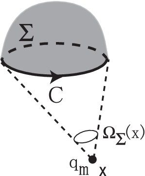
For , thus, is the (normalized) solid angle ( divided by the total solid angle ):
| (6.263) |
For , the magnetic contribution in the Wilson loop operator reads
| (6.264) |
For , the Wu-Yang configuration
| (6.265) |
leads to the magnetic-monopole density
| (6.266) |
where we have used
| (6.267) |
This corresponds to a magnetic monopole with a unit magnetic charge located at the origin. Hence, we obtain the contribution of a magnetic monopole to the Wilson loop operator:
| (6.268) |
Therefore, gives a non-trivial contribution:
| (6.269) |
for a half-integer from a magnetic monopole with a unit magnetic charge at the origin, since for the upper or lower hemisphere . This is also the case for a magnetic monopole at an arbitrary point on the minimal surface spanned by the Wilson loop . This result does not depend on which surface bounding is chosen in the non-Abelian Stokes theorem.
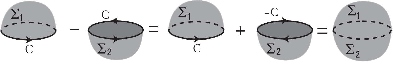
In general, we can show that the magnetic charge obeys the Dirac quantization condition:
| (6.270) |
In fact, the Dirac quantization condition for the magnetic charge is obtained from the condition: the non-Abelian Stokes theorem does not depend on the surface which is chosen for spanning the surface bounded by the loop , remembering that the original Wilson loop is defined for a given closed loop . The difference of the argument must be an integer multiple of :
| (6.271) |
where we have used . Thus, the Wilson loop operator can probe gauge-invariant magnetic monopole with the magnetic charge subject to the Dirac quantization condition. See Fig. 14.
For an ensemble of point-like magnetic charges located at () represented by
| (6.272) |
we have a geometric representation:
| (6.273) |
The magnetic monopoles in the neighborhood of the Wilson surface () contribute to the Wilson loop 6464 64 This helps us to understand the N-ality dependence of the asymptotic string tension. See [63].
| (6.274) |
Here, gives a non-trivial contribution, i.e., a center element:
| (6.275) |
This result does not depend on which surface bounding is chosen in the non-Abelian Stokes theorem. [This helps us to understand the N-ality dependence of the asymptotic string tension.] Here the magnetic flux from a magnetic monopole is assumed to be distributed isotropically in the space. However, the contribution of a magnetic monopole to the Wilson loop average depends on the location of the monopole relative to the Wilson loop.
6.7.2 magnetic monopole
In the four-dimensional case , is one-form with the component:
| (6.276) |
and is also one-form, i.e., magnetic current:
| (6.277) |
The magnetic current is conserved, .
Note that agrees with the four-dimensional solid angle given by
| (6.278) |
Consequently, we have for ,
| (6.279) |
For an ensemble of magnetic monopole loops ():
| (6.280) |
we obtain
| (6.281) |
where is the linking number between the surface and the curve :
| (6.282) |
Here the curve is identified with the trajectory of a magnetic monopole and the surface with the world sheet of a hadron (meson) string for a quark-antiquark pair. See Fig. 15.

Thus we have shown that the Wilson loop operator is a probe of the magnetic monopole defined in the gauge invariant way in the pure Yang-Mills theory even in the absence of any scalar field. Therefore, calculating the Wilson loop average reduces to the summation over the contributions coming from the distribution of magnetic monopole charges () or currents () with the geometric factor, the solid angle () or linking number (). Therefore, we do not need to use the Abelian projection to define magnetic monopoles in Yang-Mills theory!
6.8 Magnetic monopole and the associated magnetic vortex
For , however, we fall in a trouble about the magnetic monopole just defined. In fact, such magnetic loops carrying the magnetic charge obeying the Dirac quantization condition (6.270) do not give non-trivial contributions to the Wilson loop, since and are integers. If the quantization condition (6.270) is naively taken at its face value, the magnetic monopole cannot be the topological defects responsible for quark confinement. In the following, we discuss how this dilemma is resolved according to [63].
To understand the area law of the Wilson loop average in -dimensional space–time,
we want to find a -dimensional geometric object such that
i) has an intersection with the Wilson loop as the one-dimensional object,
ii) has relevance to the magnetic-monopole current as the -form .
In what follows, we consider how the magnetic flux emanating from the magnetic monopole behaves in the vacuum. We first consider the case. Suppose that the magnetic current has the support on a loop in dimensions:6565 65 In what follows, we extensively use the techniques developed in constructing a continuum analogue of the maximal center gauge and center projection by Engelhardt and Reinhardt [113].
| (6.283) |
where is a real number representing the magnetic flux carried by the magnetic current . The magnetic charge is defined by
| (6.284) |
where denotes a parameterization of the 3-dimensional volume and is the dual of the 3-dimensional volume element :
| (6.285) |
First of all, we look for the dual field strength representing the magnetic flux, which has the support on a two-dimensional surface bounding the loop , as the support of the magnetic current , so that
| (6.286) |
Such a solution is given by
| (6.287) |
In fact, it satisfies the equation:
| (6.288) |
where we have used the Stokes theorem in the last step.
Next, we proceed to obtain the gauge potential giving the field strength whose dual satisfies (6.287):
| (6.289) |
such that has the support only on the open set , the three-dimensional volume6666 66 The precise position of the open set is irrelevant for the value of the Wilson loop as shown below. In fact, the open set can be deformed arbitrarily by singular gauge transformations in such a way that its boundary representing the position of the magnetic flux of the vortex is fixed. whose boundary is : . The gauge field is called the ideal vortex field. Note that is cast into
| (6.290) |
where we have used the Gauss (Stokes) theorem in the first equality. Therefore, the gauge potential is determined up to a gauge transformation:
| (6.291) |
6.8.1 -dimensional case


We now proceed to consider the general -dimensional case. In dimensions, the magnetic current is a -form with the support on a closed -dimensional subspace :
| (6.292) |
First, we consider the dual field strength representing the magnetic flux, which has the support on an open -dimensional surface bounding a closed -dimensional subspace , , as the support of the magnetic current so that
| (6.293) |
See Fig. 16. In the similar way to the above, we find that a solution is given by
| (6.294) |
Next, we consider the ideal vortex field , giving the field strength field :
| (6.295) |
such that has the support only on the -dimensional volume whose boundary is : . We find such an explicit (singular) gauge field representation in space–time dimensions:
| (6.296) |
where is the -dimensional hypersurface (the string, surface, or volume in and , respectively) parameterized by , and is the dual of the surface element :
| (6.297) |
The volume element defines an orientation of the vortex. In general, two different orientations of vortices can be distinguished. Note that the ideal vortex field must be singular. Otherwise, the magnetic current becomes trivial , since .
It will be shown later that when the hypersurface of the ideal vortex configuration intersects with a Wilson loop , the ideal vortex contribute a center group element to the Wilson loop operator. The boundary gives the location of the thin vortex to which the ideal vortex configuration is gauge equivalent.
The ideal vortex field is not unique as mentioned above. Actually, the ideal vortex field can be gauge transformed to a thin vortex field which has the support only on the boundary of :
| (6.298) |
so that carries the same magnetic flux located on as that carried by . In fact, for , agrees with , since . In other words, and are gauge equivalent.
It is shown that such a gauge transformation is given by
| (6.299) |
where is the solid angle taken up by the volume when viewed from :
| (6.300) |
with being the area of the unit sphere in dimensions, e.g., , . The solid angle defined in this way is normalized to unity for a point inside the volume . Note that the solid angle is defined with a sign depending on the orientation of as rays emanating from pierce . A deformation of keeping its boundary fixed leaves the solid angle invariant unless crosses . When crosses , the solid angle changes by an integer.6767 67 Whether the flux of a vortex is electric or magnetic depends on the position of the dimensional vortex surface in -dimensional space–time. For example, in the vortex defined by the boundary of a purely spatial 3-dimensional volume carries only electric flux, which is directed normal to the vortex surface . On the other hand, a vortex defined by a volume evolving in time represents at a fixed time a closed loop and carries the magnetic flux, which is tangential to the vortex loop [113].
It is easy to check that the solid angle is rewritten as
| (6.301) |
by using the Green function of the -dimensional Laplacian defined by
| (6.302) |
which has the explicit form:
| (6.303) |
Now we show that the thin vortex field manifestly depends only on the boundary where the magnetic flux associated with the vortex located:
| (6.304) |
where is the dual of the volume element:
| (6.305) |
The ideal vortex field has support only on and hence it vanishes outside the volume , i.e., for . Therefore, outside the volume , i.e., , the thin vortex field is the pure gauge due to (6.298):
| (6.306) |
which implies the vanishing field strength outside the volume . This is reasonable, because the magnetic flux is contained in the vortex sheet .
The derivation of (6.298) and (6.304) is as follows. By using (6.301), we obtain
| (6.307) |
We have the decomposition:
| (6.308) |
following from the identity:
| (6.309) |
which is consistent with . This is used to rewrite the pure gauge form into
| (6.310) |
where we have used the definition of the Green function and the Stokes theorem in the second equality. In other words, the thin vortex field is the transverse part of the ideal vortex .
Finally, we find that the surface integral of over bounded by the Wilson loop is equivalent to the line integral of along the closed loop :
| (6.311) |
since the contribution from the last term vanishes for any closed loop . Then the line integral is cast into
| (6.312) |
6.8.2 vortex


For , in particular, the magnetic-monopole current is given by
| (6.313) |
the ideal vortex field with the support on the surface is written as
| (6.314) |
and the thin vortex field with the support on the closed loop is written as
| (6.315) |
By using (6.312), the line integral reads
| (6.316) |
where we have used the fact that the first term vanishes in the second to last equality, since it is the line integral on a closed loop due to the Stokes theorem.
Here is the intersection number between the Wilson surface (the string world sheet) and the vortex loop .
| (6.317) |
There are three equivalent descriptions. See Fig. 17. The intersection number between the Wilson surface and the vortex loop is equal to the intersection number between the Wilson loop and the vortex sheet , which is equal to the linking number between the the Wilson loop and the vortex loop . The intersection numbers and the linking number are integer valued:
| (6.318) |
In dimensional space–time, the contribution to the Wilson loop operator from the vortices is estimated as the factor:
| (6.319) |
If the magnetic flux carries a unit of the magnetic flux according to the quantization condition:
| (6.320) |
then a vortex as the tube of the magnetic flux contributes the factor (an element of the center group) to the Wilson loop operator:
| (6.321) |
This becomes non-trivial only when is a half-integer, , since the intersection number and the linking number are integers, . This result is consistent with the estimate obtained from the magnetic monopole (6.273). This is the most non-trivial contribution, which corresponds to the half of the total magnetic flux emanating from a point magnetic charge.
This is consistent with the claim that a center vortex configuration will appear (after Abelian projection) as a chain of monopoles alternating with antimonopoles, i.e., monopole-antimonopole chain. If this is the case, then the monopole flux is not distributed symmetrically on the Abelian-projected lattice, in contrast to the situation one might expect in a Coulomb gas. Rather, it is collimated in units of along the vortex line [48, 78, 80]. If this picture is correct, then a vortex sheet on , a vortex line on , and the magnetic monopoles on have the mutual positional relation as shown in Fig. 18. Here the vortex line is non-orientable. Otherwise, the magnetic monopoles do not exist, since the orientable vortex loop has no boundary .
6.8.3 vortex


The above consideration can be extended to higher dimensions. For , is a three-dimensional volume and its boundary is a closed two-dimensional surface . If is an oriented closed surface, then its boundary is empty, and hence the magnetic current does not exist in this case, since its support vanishes. Therefore, for the non-vanishing magnetic current to exist in the boundary of , the vortex surface must be non-oriented. For , we find
| (6.322) |
where we have used the fact that the second term vanishes due to the Stokes theorem for obtaining the last result. Therefore, the line integral is rewritten as
| (6.323) |
in terms of the intersection number between the world sheet of the hadron string and the vortex sheet in dimensions. It is known that the intersection number is equal to the linking number between the Wilson loop and the vortex sheet , see Fig. 19:
| (6.324) |
Thus the thin vortex contributes to the Wilson loop in the fundamental representation:
| (6.325) |
In general, is a complex number of modulus one, i.e., an element of . In the case of gauge group, the magnetic charge measured by the Wilson loop is subject to the Dirac quantization condition:
| (6.326) |
If the magnetic flux obeys the quantization condition with an additional factor :
| (6.327) |
then reduces to
| (6.328) |
Therefore, reduces to the center element of :
| (6.329) |
only when
| (6.330) |
In the case of gauge group, it has been shown [62] that the magnetic charge measured by the Wilson loop is subject to the quantization condition:
| (6.331) |
which is analogous to the Dirac type, but different from it. Suppose that the magnetic flux obeys the fractional quantization condition:
| (6.332) |
Then its contribution to the Wilson loop is written as
| (6.333) |
where
| (6.334) |
The center of is . For to belong to the center of , i.e., , must take the fractional number except for a trivial case :
| (6.335) |
just as the aforementioned case with the center subgroup , when . See Fig. Fig. 20. This may be related to the fact that each self-intersection point of a vortex surface contributes () to the Pontryagin index [113].
Finally, we consider the relationship between center vortices and our gauge-invariant vortices for case. The center vortex is obtained by replacing the magnetic flux with the diagonal matrix :
| (6.336) |
which indeed leads to the non-trivial elements of the center group :
| (6.337) |
where corresponds to the trivial element . Thus the center vortices are replaced by our gauge-invariant vortices carrying the fractional magnetic flux .
If this observation is correct, the magnetic part of the Wilson loop with an additional fractional factor :
| (6.338) |
will reproduce the string tension for any (), just as confirmed for gauge group in [27]. This is a conjecture derived in the paper [63]. This is consistent with the center vortex mechanism for quark confinement. However, it will be rather difficult to identify the vortex structure in case in numerical simulations. For the vortex surfaces for , , may branch and the superimposed magnetic fluxes in general also modify the type of vortex flux, i.e., its direction in color space. See e.g., [115].
The () vortex condensation theory for quark confinement put forward by ’t Hooft [73], Mack [74], Cornwall [75] and by Nielsen, Olesen and Ambjorn [76] (“Copenhagen vacuum”) is that the QCD vacuum is presumed to be filled with closed magnetic vortices, which carry magnetic flux in the center of the gauge group, and have the topology of tubes for or surfaces for of finite thickness.
The effect of creating a center vortex linked to a given Wilson loop is as follows: If the area of a Wilson loop is pierced by such vortices, the value of the Wilson loop in the gauge theory is multiplied by a factor of , an element of the gauge group center :
| (6.339) |
Quantum fluctuations in the number of vortices linked to the Wilson loop can be shown to lead to an area law fall-off, assuming that center vortex configurations are condensed in the vacuum. The area law is attributed to random fluctuations in the number of vortices piercing the Wilson loop. From the viewpoint of the Aharonov-Bohm effect, see e.g., [116].
6.9 Vortex picture toward the area law

The vortex condensation picture gives an easy way to understand the area law. Let us assume that the vacuum is filled with percolating thin vortices. Suppose that random vortices intersect a plane of area . See Fig. 21. For simplicity, we consider the gauge group in what follows. Each intersection multiplicatively contributes a factor to the Wilson loop average and intersect within the loop take the value . Then the probability that of the intersections occur within an area spanned by a Wilson loop is given by .
Summing over all possibilities with the proper binomial weight yields
| (6.340) |
where
| (6.341) |
where has been eliminated in favor of the planar vortex density . The limit of a large is taken with a constant . Thus one obtains an area law for the Wilson loop average with the string tension determined by the vortex density .
The crucial assumption in this argument is the independence of the intersection points. The asymptotic string tensions are zero for all integer- representations (with -ality or “biality” being equal to ), while they are nonzero and equal for all half-integer representations (with -ality or “biality” being equal to ). This is the asymptotic string tension. See section 10.5.2 for the string tension in the intermediate distance region.
6.10 magnetic monopole
For concreteness, we discuss the case. The gauge transformation of the Yang-Mills field by a group element is given by
| (6.342) |
We can express a group element of explicitly by the Euler angles:
| (6.343) |
where are the Pauli matrices. Then the inhomogeneous term is parameterized as
| (6.344) |
which has the Lie-algebra value:
| (6.345) |
First, we examine the Abelian projection picture for magnetic monopoles in Yang-Mills theory. It is easy to show that an identity holds for :
| (6.346) |
Then the Abelian field strength of the diagonal part reads
| (6.347) |
where we have defined by
| (6.348) |
Using the above Euler-angle expression (6.345) for , we obtain
| (6.349) |
Now we show that represents the magnetic monopole contribution to the diagonal field strength . Note that is generated from the off-diagonal components, .
For , the magnetic charge is calculated as the volume integral:
| (6.350) |
from the magnetic current:
| (6.351) |
By using the Stokes (Gauss) theorem, the volume integral is replaced by the surface integral over the two-dimensional closed surface which is the boundary of the three-dimensional volume :
| (6.352) |
We can identity the first part of right-hand-side of (6.347) with the the magnetic monopole part, while the second part with the Dirac string part in the Yang-Mills theory.6868 68 See Appendix of [53] for more details. This is clearly seen by the explicit calculation, since we can rewrite (6.347) as
| (6.353) |
For the magnetic charge, the contribution from the magnetic monopole part is given by
| (6.354) |
while the contribution from the Dirac string part is
| (6.355) |
The first contribution (6.354) to the magnetic charge leads to the quantized magnetic charge. This is because the integrand is the Jacobian from to . (See (6.371) for the details of the calculation.) Then (6.354) gives the magnetic charge satisfying the Dirac quantization condition,
| (6.356) |
This result is consistent with the non-trivial Homotopy group:
| (6.357) |
In the second contribution (6.355) to the magnetic charge, if we choose using the residual gauge invariance, then the Dirac string appears on the negative axis, i.e., . In this case, the surface integral reduces to the line integral along a closed path around the string using the Stokes theorem:
| (6.358) |
This gives the same result (6.355) but with the minus sign, which is consistent with the non-trivial Homotopy group:
| (6.359) |
Actually, two description are equivalent, as suggested from the mathematical identity:
| (6.360) |
If the contribution from is completely neglected, then (6.346) implies that the field strength of is given by
| (6.361) |
Note that the original Yang-Mills theory does not have the magnetic monopole solution. However, if we adopt the MA gauge, that is to say, we partially fix the gauge symmetry to and retain the residual gauge symmetry, then the theory can have singular configuration. This is a reason why the magnetic monopole appears in the Yang-Mills theory which does not have Higgs field. The existence of the Dirac string in the right-hand side of (6.361) reflects the fact that the field strength does contain the magnetic monopole contribution. We have obtained a gauge theory with magnetic monopoles starting from the Yang-Mills theory. Therefore, the MA gauge enables us to deduce the magnetic monopole without introducing the scalar field, in contrast to the ’t Hooft-Polyakov monopole.

Second, we examine magnetic monopoles from the picture of the CDG decomposition. The color field has the the target space (See Fig. 22):
| (6.362) |
The existence of magnetic monopole is consistent with a non-trivial Homotopy class of the map :
| (6.363) |
The magnetic charge obey the Dirac quantization condition:
| (6.364) |
We show that the color field generates the magnetic charge subject to the Dirac quantization condition. The color field is expressed in the Lie-algebra form:
| (6.365) |
or the vector form:
| (6.366) |
By using the expression (6.343) for , the color field is parameterized by two polar angles on the target space :
| (6.367) |
The gauge-invariant magnetic current is obtained from the gauge-invariant field strength:
| (6.368) |
In fact, the field strength is written in the manifestly gauge-invariant form (3.50):
| (6.369) |
We use the parameterization of the last term:
| (6.370) |
Taking into account the fact that is the Jacobian from to parameterized by , thus, we obtain the Dirac quantization condition for the magnetic charge:
| (6.371) |
since is the surface element on and a surface of a unit radius has the area . Hence gives a number of times is wrapped by a mapping from to . This fact is understood as the Homotopy group: .
We can introduce the Abelian potential for the magnetic monopole:
| (6.372) |
In fact, the field strength of the potential agrees with :
| (6.373) |
Therefore, we call the magnetic potential. Therefore, non-vanishing magnetic charge is derived only when the magnetic potential has singularities. Otherwise, the magnetic current is identically zero due to the Bianchi identity.
| (6.374) |
where we have calculated the line integral around the infinitesimal closed loop around the Dirac string, i.e., line of singularities on the positive or negative axis where for . See Fig. 1.
Finally, we discuss the gauge reducing to the Abelian projection. For , if we choose a special gauge, unitary-like gauge, in which the color field has the uniform color direction everywhere:
| (6.375) |
then the gauge-invariant field strength reduces to the Abelian form:
| (6.376) |
and the Wilson loop operator reduces to the “Abelian-projected” form:
| (6.377) |
Therefore, the Abelian projection is reproduced from the gauge-invariant treatment as a special limit of taking the unitary-like gauge (6.375).
6.11 magnetic monopole
We examine the quantization condition for the magnetic charge. The magnetic current (-form) is defined using the gauge-invariant field strength (two-form) by
| (6.378) |
For , the magnetic current reads
| (6.379) |
Hence, the magnetic charge is defined by
| (6.380) |
In the case, the two kinds of gauge-invariant magnetic-monopole currents are given by the field strength: The calculations can be done by using the Lie algebra form:
| (6.381) |
which is easier than the vector form:
| (6.382) |
where and are defined by
| (6.383) |
Here we have used the field strength for the maximal option obtained in section 5.7.1:
| (6.384) |
Then it is shown later that one can define two gauge-invariant charges and which obey the different quantization conditions [10]:
| (6.385) |
The existence of magnetic monopole characterized by two integers and is consistent with a fact that the map defined by
| (6.386) |
has the nontrivial Homotopy group:
| (6.387) |
On the other hand, the existence of magnetic monopole characterized by an integer is consistent with a fact that the map defined by
| (6.388) |
has the nontrivial Homotopy group:
| (6.389) |
However, it should be noted that the Wilson loop in the fundamental representation does not distinguish and , and can probe only the combinations represented by as follows. For and ,
| (6.390) |
for and ,
| (6.391) |
and, in particular, for and ,
| (6.392) |
These quantization conditions for are reasonable because they guarantee that the Wilson loop operator defined originally by the closed loop should not depend on the choice of the surface bounded by the loop when rewritten in the surface integral form by the non-Abelian Stokes theorem, just as in the case.
| (6.393) |
The quantization condition is written as
| (6.394) |
The diagonal element leads to the relationship between the magnetic charge and the weight vector of the fundamental representation:
| (6.395) |
For in the minimal option, the color field is defined by the Lie algebra form:
| (6.396) |
using and an group element . The color field is also written in the vector form:
| (6.397) |
A group element of is parameterized by using eight angles as6969 69 See e.g., [117, 118] for more details.
| (6.398) |
By using the expression (6.398) for the element , and are represented as follows
| (6.399) |
| (6.400) |
In particular, by adopting one of the simplest choice of parameters [119]
| (6.401) |
the quantization conditions (6.385) are obtained from an explicit expression of the color field written in terms of two angles [21]:
| (6.402) |
In fact, the Lie algebra form of the color field is obtained by substituting the components (6.402) into
| (6.403) |
Then another color field is obtained
| (6.404) |
Using the unit vectors in the directions, we find
| (6.405) |
which are used to calculate the surface integration over the sphere:
| (6.406) |
In other words, the gauge-invariant magnetic fields are obtained as
| (6.407) |
6.12 non-Abelian magnetic monopole and the magnetic charge quantization condition
The magnetic charge is defined by the total magnetic flux sourced by the magnetic monopole integrated over a sphere centered on the magnetic monopole, which should be equal to . On the other hand, the electric coupling of the gauge field with the matter in the fundamental representation of is through the minimum coupling constant . In fact, the magnetic flux sourced by a magnetic monopole for is calculated as
| (6.408) |
| (6.409) |
which leads to
| (6.410) |
Here is the electric coupling constant, which enters the Lagrangian as
| (6.411) |
where is an doublet matter fields. This means the minimum electric charge :
| (6.412) |
Thus the magnetic charge is given by the minimum electric charge :
| (6.413) |
which coincides with the Dirac minimum quantum of magnetic charge.
For in the minimal option corresponding to , the magnetic flux sourced by a magnetic monopole is calculated as
| (6.414) |
This means that the minimum magnetic charge is
| (6.415) |
As enters the Lagrangian in the covariant derivative
| (6.416) |
where the factor comes from the normalization of the Gell-Mann matrix . This means the minimum electric charge :
| (6.417) |
Thus the magnetic charge of the magnetic monopole is given by the minimum electric charge :
| (6.418) |
which is one half of the Dirac minimum quantum of magnetic charge.
Similarly, for in the minimal option corresponding to , the magnetic flux sourced by a magnetic monopole is calculated as
| (6.419) |
This means that the minimum magnetic charge is
| (6.420) |
As enters the Lagrangian in the covariant derivative
| (6.421) |
where the factor comes from the normalization of the Gell-Mann matrix . This means that the minimum electric charge is given by
| (6.422) |
Thus the magnetic charge of the magnetic monopole is given by by the minimum electric charge :
| (6.423) |
which is of the Dirac minimum quantum of magnetic charge. This factor of is the degree of the embedding of the fundamental group of the unbroken into that of the unbroken gauge group. 7070 70 See e.g., [120, 121] for more details.
7 Infrared dominant field modes and the high-energy relevant field modes
In order to establish the dual superconductivity as a gauge-invariant concept, we should cure various shortcomings associated to the MA gauge.
7.1 Gauge-independent “Abelian” dominance for the Wilson loop operator
We pay attention to the Wilson loop operator for the Yang-Mills gauge connection :
| (7.1) |
We consider the decomposition of the gauge field into two pieces and :
| (7.2) |
so that the resulting new field variables and have the following remarkable property: For the gauge group ,
- (a)
The Wilson loop operator defined in terms of the original Yang-Mills field can be reproduced by the restricted field variable alone and the remaining field variable is redundant for the Wilson loop operator:
(7.3) where is defined by
(7.4) - (b)
The non-Abelian field strength of the restricted field has the form
(7.5) If the color field transforms according to the adjoint representation, just like under the gauge transformation, then the magnitude is gauge invariant.
Once the Wilson loop operator is rewritten in terms of the surface integral over the surface bounded by the closed loop , the the Wilson loop operator is rewritten in terms of the invariant “Abelian” field strength derived from the field strength of the restricted field variable :
(7.6) where is defined by
(7.7) for any representation of specified by a half-integer .
The set of statements (a) and (b) represents a gauge-independent “Abelian” dominance or the restricted field dominance for the Wilson loop operator (in the operator level), which we call the strong Abelian dominance. Some remarks are in order.
- 1.
The strong “Abelian" dominance holds for arbitrary closed loop , irrespective of its shape and size.
- 2.
The strong “Abelian" dominance in the above sense does not hold on the lattice. It is obtained only in the continuum limit of the lattice spacing going to zero , i.e., after removing the regularization. Therefore, there exists some deviation on a lattice coming from non-zero lattice spacing . 7171 71 In [64], the result obtained for in the continuum formulation was extended to the on the lattice and in the continuum. A constructive proof was given by deriving the lattice regularized version of the non-Abelian Stokes theorem and the lattice versions of the gauge field decomposition which have been constructed and developed for in [27, 28] and for in [30, 31] according to the continuum versions given in [18] and [24], respectively. The constructive approach enables one to compare the result of numerical simulations with the theoretical consideration, or even give a numerical proof of the non-Abelian Stokes theorem. It is possible to give a formula estimating a systematic error of the lattice Wilson loop operator from the continuum Wilson loop operator due to the non-zero lattice spacing . In fact, an estimation of this deviation was given up to . Moreover this will shed new light on the role of the MA gauge for the Abelian dominance on a lattice.
- 3.
The strong “Abelian" dominance does NOT immediately imply the dominance of the Wilson loop average for arbitrary closed loop :
(7.8) For the large loop , this equality called the infrared Abelian dominance is expected to hold. The reason is explained below (7.36).
Th restricted field variable in the new formulation corresponds to the “diagonal" gluon field variable in the Abelian projection scheme, while the remaining field variable to the “off-diagonal" gluon field variable. The color field represents a space–time-dependent, i.e., local embedding of the Abelian direction into the non-Abelian color space and hence the Abelian direction can vary from point to point of space–time, while in the Abelian projection the Abelian direction is fixed over the whole space–time.
The general case is more involved from the technical points of view. For the gauge group , , we define the strong Abelian dominance for the Wilson loop operator in the fundamental representation, related to the gauge-independent “Abelian” dominance or the restricted field dominance for the Wilson loop average :
- (a)
The Wilson loop operator defined in terms of the original Yang-Mills field can be reproduced by the restricted field variable alone and the remaining field variable is redundant for the Wilson loop operator:
(7.9) where is defined by
(7.10) - (b)
Once the Wilson loop operator is rewritten in terms of the surface integral over the surface bounded by the closed loop , the the Wilson loop operator is rewritten in terms of the invariant “Abelian” field strength derived from the field strength of the restricted field variable :
(7.11) where is defined by
(7.12)
The decomposed fields and are determined by solving the following defining equations (I) and (II), once the color (direction) field is given:
(I) is a covariant constant in the background :
| (7.13) |
(II) does not have the -commutative part:
| (7.14) |
where denotes the maximal stability subgroup of the gauge group which is determined by specifying the highest-weight state of the representation of the Wilson loop.
A set of conditions:
| (i) | (7.15) | |||
| (ii) | (7.16) |
is a sufficient condition for the gauge-independent “Abelian" dominance represented by (a) and (b) for the Wilson loop operator in any representation of and in the fundamental representation for . In fact, the condition (ii) guarantees (a), while the condition (i) guarantees (b).
| (i) | (7.17) |
This statement will be verified shortly. The proofs of (a) and (b) are given in section 6.
For , the two conditions (7.15) and (7.16) agree with the first and second defining equations respectively for specifying the conventional Cho-Duan-Ge-Faddeev-Niemi (CDGFN) decomposition.Therefore, the CDGFN decomposition is a sufficient condition for the gauge-independent Abelian dominance for the Wilson loop operator.7272 72 This fact that the CDGFN decomposition leads to the Abelian dominance in the strong sense was pointed out in the continuum formulation through the non-Abelian Stokes theorem in [122]. In other words, the strong Abelian dominance gives a raison d’etre and a physical meaning of gauge covariant decomposition of the gauge field variable a lá CDGFN.
The general () case is more involved than the case from the technical points of view. For , a set of conditions (i) and (ii) follows from a set of the defining equations (I) and (II) which specify the gauge field decomposition, including the CDGFNS decomposition for as a special case. In the minimal option, the gauge field decomposition (7.2) has been achieved by way of a single color field for . Therefore, the strong Abelian dominance in the Wilson loop is an immediate consequence of the gauge field decomposition.
In fact, the defining equation (II) for :
| (7.18) |
leads to the condition (ii):
| (7.19) |
where we have used an identity: . The condition (i) agrees with the first defining equation (I) for the decomposition .
| (I) | (7.20) |
Now we proceed to show the relation (7.17). First, we consider the implication of the condition (ii). The Wilson loop operator has the pre-NAST:
| (7.21) |
with the one-form defined by (see section 6.2)
| (7.22) |
where we have defined the traceless field
| (7.23) |
and the normalized and traceless field .
| (7.24) |
For the decomposition , the one-form is decomposed as
| (7.25) |
Therefore, the condition (ii) means that does not depend on and that can be replaced by in the Wilson loop operator. This is the statement (a).
Next, we consider the implication of the condition (i). For a while, we use the different notation, and , to avoid the confusion in the commutator . The commutator between and a color field is calculated as
| (7.26) |
using
| (7.27) |
Indeed, this is shown as follows.
| (7.28) |
where we have used the Jacobi identity in the second equality and the relation: for an arbitrary function in the third and the last equalities. Thus, if and satisfies the condition (i):
| (7.29) |
then the field strength of the field and commute:
| (7.30) |
For , (7.30) means that the field strength of the field has only the “Abelian” part proportional to :
| (7.31) |
since is traceless and cannot have a part proportional to the unit matrix. This yields the stronger sense of “Abelian dominance”.
For , the above argument is more involved from the technical points of view. In the () case, is not proportional to , even if (7.30) holds:
| (7.32) |
is equal to the -commutative, i.e., -commutative part:
| (7.33) |
where are a set of generators of the Lie algebra of , which commute with .
However, the properties (a) and (b) are directly checked by using the explicit expression of decomposed fields which are uniquely determined by solving the defining equation (I) and (II).7373 73 See Kondo [62] and Kondo, Shinohara and Murakami [24] for the full details.
Therefore, once the Wilson loop operator is rewritten into the surface integral form through the non-Abelian Stokes theorem using the coherent state, it is represented by the ( gauge-invariant) “Abelian” field strength constructed from the field strength of the restricted field :
| (7.34) |
Thus we have obtained a gauge-independent “Abelian” dominance in the continuum form:
| (7.35) |
where is defined in a gauge-covariant and gauge-independent way and becomes gauge invariant and hence gauge independent.
Thus we have obtained a sufficient condition for realizing the gauge-independent “Abelian" dominance in the Wilson loop operator. However, it should be remarked that the strong “Abelian" dominance holds in the operator level for the Wilson loop operator itself with arbitrary shape and size. Whereas, the ordinary infrared Abelian dominance refers to the expectation value:
| (7.36) |
The strong Abelian dominance for the Wilson loop operator, , does not necessarily imply the dominance of the Wilson loop average , which is defined by
| (7.37) |
Here the original integration measure and the action cannot be written in term of the restricted field alone: In fact, the action has the cross term or the interaction term between and , i.e., , as shown in section 5.7.3. Therefore, the infrared Abelian dominance in the string tension confirmed numerically from the Wilson loop average does not immediately follows from the strong “Abelian" dominance just defined. In the infrared region, however, the field decouples from the theory and the effect of the cross term becomes negligible. According to the numerical simulations, indeed, there exists a non-trivial correlation between and , but the correlation function and fall off rapidly as the distance between and increases.7474 74 For case, see Shibata et al. [28]. For in the minimal option, see Shibata et al. [148]. For a sufficiently large loop , finally, the strong “Abelian" dominance for the Wilson loop operator reduces to infrared Abelian dominance for the Wilson loop average.
Finally, we point out that the conventional Abelian projection is reproduced as a special case for the uniform color field:
| (7.38) |
the defining equation (II) implies that is the off-diagonal matrix: , while (I) implies that is the diagonal matrix: . Thus, reduces just to the Cartan decomposition. Then the field strength reduces to the usual definition for the diagonal gauge field : . The strong Abelian dominance reads
| (7.39) |
Therefore, the color field plays the role of recovering color symmetry which is lost by a global (i.e., space–time independent or uniform) choice of the Abelian direction taken in the conventional approach, e.g., the MA gauge.
7.2 Wilson loop average in the new formulation
The Wilson loop average is defined by
| (7.40) |
with the partition function by omitting the gauge fixing procedure to simplify the expression. The pre-NAST (7.21) for the Wilson loop operator tells us that
| (7.41) |
Inserting the unity:
| (7.42) |
yields
| (7.43) |
Thus, in the reformulated Yang-Mills theory in which , , are regarded as the independent field variables, the Wilson loop average is written
| (7.44) |
where the Yang-Mills action is rewritten in terms of new variables using (7.2) and (6.205),
| (7.45) |
and the integration measure is finally transformed to
| (7.46) |
The new partition function is introduced:
| (7.47) |
It is shown that
- (i)
the reduction condition is rewritten in terms of new variables:
(7.48) - (ii)
- (iii)
In the previous section, the Wilson loop operator has been exactly rewritten in terms of the gauge-invariant magnetic current and the electric current . This shows that the Wilson loop operator can be regarded as a probe of magnetic monopoles. In this section, moreover, we have succeeded to connect the Wilson loop average with magnetic monopoles which is supposed to be a basic ingredient to cause dual superconductivity as a promising mechanism of quark confinement. In fact, (7.44) tells us what quantity we should examine to see the magnetic monopole contribution to the Wilson loop average. This equation is important to give a connection between our formulation and magnetic monopole inherent in the Wilson loop in order to show quark confinement. In fact, we give numerical calculations of the potential based on the lattice version of (7.44) given later. The magnetic monopole can be extracted from the restricted field alone.
7.3 Extracting the independent field degrees of freedom
According to the non-Abelian Stokes theorem, the Wilson loop operator is rewritten in terms of and the color field , and does not depend on the field variable . Therefore, we can integrate out the field variable in principle, if the action and the integration measure are rewritten in terms of the new variables. In order to perform the integration over , the independent field degrees of freedom are to be identified in the integration measure in calculating the Jacobian, while the action can be written in terms of independent degrees of freedom by substituting the decomposition. Among the components (), the component () in the basis are regarded as the independent degrees of freedom.
For , we use and (F.7) to calculate the covariant derivative of the basis in the background :
| (7.50) |
where we have introduced
| (7.51) |
and used the relation:
| (7.52) |
Here is called the magnetic potential. The derivation of the relation (7.52) is given in Appendix J.
In the minimal option of , we find
| (7.53) |
This is derived as follows. We use (5.194) and (F.1) to calculate
| (7.54) |
where we have used
| (7.55) |
Then the covariant derivative of in the background reads
| (7.56) |
Hence the second covariant derivative reads
| (7.57) |
Thus the piece quadratic in is rewritten as
| (7.58) |
where we have defined
| (7.59) |
Here we have used the normalization convention:
| (7.60) |
In the minimal option of , the quartic term in reads
| (7.61) |
where we have used .
Thus the Yang-Mills Lagrangian density in the minimal option (5.245) reads
| (7.62) |
where we have defined
| (7.63) |
with
| (7.64) |
For , in particular, , ,
| (7.65) |
where we have used .
The term quadratic in is further rewritten using the complex-valued field defined by :
| (7.66) |
In the above derivation, we have used the reduction condition. In this basis, the reduction condition has the same form as the conventional MA gauge fixing condition:
| (7.67) |
since (7.56) yields
| (7.68) |
In the maximal option of , the diagonal part and the off-diagonal part in the conventional Abelian projection are identified with and respectively:
| (7.69) |
For , in particular, we find
| (7.70) |
But, this does not mean that the reduction condition agrees with the MA gauge. Recall that the reduction condition is introduced to eliminate the extra degrees of freedom in the new reformulation to obtain the same independent degrees of freedom as the original one. Therefore, the above Lagrangian is still invariant under the local gauge transformation, and we can impose any gauge fixing condition, if we want to do so. The above formulation reduces to the MA gauge, only when we set the color field to be uniform in the maximal option, and hence the other bases are also fixed. The minimal option for () does not agree with the MA gauge, even in this limit.
7.4 Integrating out the infrared non-dominant field
We proceed to integrate out the field in the functional integration (7.47). For this purpose, we have already rewritten the action (7.61) of the reformulated Yang-Mills theory using the independent variables .
First, we neglect the term quartic in . The effect of the quartic term will be included later in section 7.6.
Second, we perform the integration over using the Gaussian (Fresnel) integration, by taking into account the fact that the Jacobian for the change of variables is trivial if the basis adopted in the above is used. In the Minkowski space–time, the integration over the field yields
| (7.71) |
while in the Euclidean space,
| (7.72) |
We have already included the reduction condition . In addition, we include the Faddeev-Popov like term associated with the reduction condition. The resulting expression [19, 20] is
| (7.73) |
Thus we obtain the effective Yang-Mills Lagrangian density in the minimal option: In the Minkowski space,
| (7.74) |
while in the Euclidean space,
| (7.75) |
For ,
| (7.76) |
Here is written in the matrix form:
| (7.77) |
The action for is simplified as
| (7.78) |
This formulation for has been already applied to the following problems.
- i)
- ii)
- iii)
derivation of a low-energy effective field theory in which the propagator of the restricted field has the Gribov-Stingl form which violates the physical positivity, explaining confinement of the restricted field [125].
- iv)
crossover between chiral-symmetry-breaking/restoration and confinement/deconfinement phase transition at finite temperature [126].
For in the maximal option, is given by
| (7.79) |
The structure constants are written in the matrix form () which are the off-diagonal matrices:
| (7.80) |
yield the diagonal matrices for the contracted structure constants:
| (7.81) |
Thus we find that is decomposed into the diagonal part and the off-diagonal part:
| (7.82) |
which is written in the matrix form (omitting the Lorentz index):
| (7.83) |
For in the minimal option, has the form
| (7.84) |
which has apparently the same form as that in the maximal option, but the explicit form is different from that, since indices are taken over different values. In fact, the structure constants are written in the matrix form:
| (7.85) |
yield the diagonal matrices for the contracted structure constants:
| (7.86) |
Other terms gives the off-diagonal matrices:
| (7.87) |
and
| (7.88) |
yields
| (7.89) |
Then
| (7.90) |
| (7.91) |
and
| (7.92) |
yields
| (7.93) |
Finally, we find that has the form:
| (7.94) |
where we have defined .
7.5 QCD at finite temperature
In this section, we give a theoretical framework to obtain a low-energy effective theory of quantum chromodynamics (QCD) toward a first-principle derivation of confinement/deconfinement and chiral-symmetry breaking/restoration crossover transitions. In fact, we demonstrate that an effective theory obtained using simple but non-trivial approximations within this framework enables us to treat both transitions simultaneously on equal footing. A resulting effective theory at finite temperature is regarded as a modified and improved form of nonlocal version of the Polyakov-loop extended Nambu-Jona-Lasinio (nonlocal PNJL) models proposed recently by Hell, Rössner, Cristoforetti and Weise [128], Sasaki, Friman and Redlich [129], and Blaschke, Buballa, Radzhabov and Volkov [130], extending the original (local) PNJL model by Fukushima [127]. The Nambu-Jona-Lasinio (NJL) model [131] is well known as a low-energy effective theory of QCD to describe the dynamical breaking of chiral symmetry in QCD (at least in the confinement phase), see e.g. [132, 133].
A novel feature obtained by our results is that the nonlocal NJL coupling depends explicitly on the temperature and Polyakov loop, which affects the entanglement between confinement and chiral symmetry breaking, together with the cross term introduced through the covariant derivative in the quark sector considered in the conventional PNJL model. The chiral symmetry breaking/restoration transition is controlled by the nonlocal NJL interaction, while the confinement/deconfinement transition in the pure gluon sector is specified by the nonperturbative effective potential for the Polyakov loop obtained recently by Marhauser and Pawlowski [134], Fischer, Maas and Pawlowski [135] and Braun, Gies and Pawlowski [136]. The basic ingredients are a reformulation of QCD based on new variables and the flow or functional renormalization group (FRG) equation of the Wetterich type in the Wilsonian renormalization group. This framework can be applied to investigate the QCD phase diagram at finite temperature and density.
The action of QCD is written in terms of the gluon field and the quark field :
| (7.95) |
where is the quark field, is the quark mass matrix, is the quark chemical potential, are the Dirac gamma matrices (), is the covariant derivative in the fundamental representation, is the QCD coupling constant, is the gluon field with generators for the gauge group () and is the field strength. In what follows, we suppress the spinor, color and flavor indices. Here is the gauge-fixing term and is the associated Faddeev-Popov ghost term.
By making use of new variables and obtained from decomposing the original Yang-Mills field:
| (7.96) |
the original QCD action is rewritten into a new form:
| (7.97) |
where we have introduced the color current in the basis :
| (7.98) |
the covariant derivative in the adjoint representation and
| (7.99) |
Here we have explicitly written the independent degrees of freedom for the fields which are to be integrated out below.
We neglect the quartic term , which will be taken into account later in section 7.6. The integration over can be achieved by the Gaussian integration:
| (7.100) |
Consequently, a nonlocal 4 fermion-interaction is generated:
| (7.101) |
where the last term in the action comes from the Faddeev-Popov determinant associated with the reduction condition (see section 4.6 and [19] for the precise form).
In order to estimate the effect of the nonlocal four-fermion interaction, we assume that the inverse is diagonal in the Lorentz indices neglecting the antisymmetric term :
| (7.102) |
Then the interaction term reads
| (7.103) |
Moreover, we consider only the diagonal parts of . 7575 75 This approximation is used just for simplifying the Fierz transformation performed below and hence it can be improved by taking into account the off-diagonal parts of if it is necessary to do so. This is achieved by the procedure
| (7.104) |
which yields
| (7.105) |
where . Then the interaction term reads
| (7.106) |
For , we use the Fierz identity [138] to rewrite the nonlocal current-current interaction as
| (7.107) |
where the are a set of Dirac spinor, color and flavor matrices, resulting from the Fierz transformation, with the property . Although the Fierz transformation induces mixings and recombinations among operators, the resulting theory must maintain the symmetries of the original QCD Lagrangian. A minimal subset of operators satisfying the global chiral symmetry which governs low-energy QCD with -flavors is the color-singlet of scalar-isoscalar and pseudoscalar-isovector operators. Thus, by restricting hereafter to
| (7.108) |
and ignoring other less relevant operators (vector and axial-vector terms in color singlet and color octet channels), we arrive at a nonlocal gauged NJL model:
| (7.109) |
This form is regarded as a gauged version of the nonlocal NJL model proposed in [128]. The function is replaced by a coupling constant times a normalized distribution :
| (7.110) |
The standard (local) gauged NJL model follows for the limiting case with .
In contrast to [128], however, and are determined in conjunction with the behavior of the Polyakov loop at temperature : using the Fourier transform of , they are expressed as
| (7.111) |
The theory given above by is able to describe chiral-symmetry breaking/restoration and quark confinement/deconfinement on an equal footing where the pure gluon part describes confinement/deconfinement transition signaled by the Polyakov loop average. We can incorporate the information on confinement/deconfinement transition at finite temperature into the quark sector through the covariant derivative and the nonlocal NJL interaction ( and ), in sharp contrast to the conventional PNJL model where the entanglement between chiral-symmetry breaking/restoration and confinement/deconfinement was incorporated through the covariant derivative alone and the nonlocal NJL interaction is fixed to the zero-temperature case. In our theory, the nonlocal NJL interaction ( and ) is automatically determined through the information of confinement/deconfinement dictated by the Polyakov loop (non-trivial gluon background), while in the nonlocal PNJL model [128] the low-momentum (non-perturbative) behavior of was not controlled by first principles and was provided by the instanton model.
For Yang-Mills theory at finite temperature , of (7.77) is written in the matrix form
| (7.112) |
where the gauge fixing condition is adopted. Here we have chosen a trivial background for the spatial component () and the uniform background for the time component with the angle variable which specifies the Polyakov loop operator. Then this leads to
| (7.113) |
where is defined by
| (7.114) |
where is the infrared cutoff function at the flow parameter used in the functional renormalization group. Then the nonlocal interaction is obtained as
| (7.115) |
whose Fourier transform is 7676 76 In what follows, we correct some errors in Kondo [126]: (82), (88), (103), (104), (105), (107). These equations should be corrected as given below, which are to be consistent with (7.115) and (7.116). But qualitative results obtained in [126] do not change by these corrections.
| (7.116) |
Note that and hence diverge at . This comes from an improper treatment of the part. To avoid this IR divergence at , we add the contribution and replace by
| (7.117) |
and
| (7.118) |
In fact, such a contribution comes in as an additional term from the terms (Note that terms are absent for ), as already mentioned before.
At (and at zero chemical potential ), QCD must be in the hadron phase where the chiral symmetry is spontaneously broken, which means that the NJL coupling constant at zero temperature must be greater than the critical NJL coupling constant :
| (7.119) |
The nonlocality function or the form factor at behaves as
| (7.120) |
and
| (7.121) |
As an immediate outcome of the resulting effective theory, this determines the temperature-dependence of the coupling constant of nonlocal NJL model. Using (7.111), we have
| (7.122) |
which lead to the NJL coupling constant normalized at :
| (7.123) |
In the presence of the dynamical quark , the Polyakov loop is not an exact order parameter and does not show a sharp change with discontinuous derivatives. Even in this case, we can introduce the pseudo critical temperature as a temperature achieving the peak of the susceptibility. Below the deconfinement temperature , i.e., , therefore, (or ), the NJL coupling constant has the temperature-dependence:
| (7.124) |
This naive estimation gives a qualitative understanding for the existence of chiral phase transition. Since is (monotonically) decreasing as the temperature increases, it becomes smaller than the critical NJL coupling constant:
| (7.125) |
Thus, the chiral transition temperature will be determined (if the chiral-symmetry restoration and confinement coexist or the chiral symmetry is restored in the confinement environment before deconfinement takes place, i.e., ) by solving
| (7.126) |
Here we have assumed that the nonlocality function gives the dominant contribution at , namely, and that the occurrence of the chiral transition is determined by the NJL coupling constant alone.
At finite temperature , the form factor reads
| (7.127) |
where we have defined and used
| (7.128) |
The form factor does not change so much around the deconfinement temperature (or ). This is reasonable since the form factor is nearly equal to the correlator , as already mentioned before. The more details can be seen in [126] .
7.6 Effect of the quartic interaction among
We can introduce the gauge-invariant mass term which is invariant under the local gauge transformation II as pointed out in [18]:
| (7.129) |
since the mass dimension two operator is invariant under the local gauge transformation:
| (7.130) |
This gauge-invariant mass term is rewritten in terms of the original variables :
| (7.131) |
under the understanding that the color field is expressed in terms of the original gauge field by solving the reduction condition. Therefore, (or and ) plays the similar role to the Stückelberg field to recover the local gauge symmetry. Note that , and are treated as independent variables after the non-linear change of variables and the mass term is a polynomial in the new variable , although they might be non-local and non-linear composite operators of the original variables .
The proposed mass term (7.129) or (7.131) for the gluon:
| (7.132) |
should be compared with the conventional gauge-invariant mass term of Kunimasa–Goto type [137]:
| (7.133) |
This mass term is non-polynomial in the Stückelberg field . This fact makes the field theoretical treatment very difficult.
It is possible to argue that there occurs a novel vacuum condensation of mass dimension–two for the field , i.e.,7777 77 We adopt the Minkowski metric . After the Wick rotation to the Euclidean region, the Minkowski metric tensor is replaced by . Therefore, we have .
| (7.134) |
and that the field acquires the mass dynamically through this condensation. A naive way to see this is to apply the mean-field like argument or the Hartree–Fock approximation to the four-gluon interaction, i.e., the quartic self-interaction among which leads to the gauge-invariant mass term for gluons and a gauge-invariant gluon mass :
| (7.135) |
Consequently, the gauge-invariant mass for the “off-diagonal” gluon is generated. Then the gluon modes decouple in the low-energy (or long-distance) region below the mass scale . Consequently, the infrared “Abelian” dominance for the large Wilson loop average follows immediately from the fact that the Wilson loop operator is written in terms of alone according to the non-Abelian Stokes theorem for the Wilson loop operator and that the Wilson loop average is entirely estimated by the restricted field alone.
The numerical simulations on a lattice [27] have demonstrated the infrared “Abelian” dominance and magnetic monopole dominance in the string tension within the compact lattice reformulation, although such phenomena were found for the first time in the MA gauge [36, 38]. In fact, the numerical simulations have shown that the string tension calculated from the magnetic part of the Wilson loop average in the reformulation of lattice Yang-Mills theory reproduces 90 95 % of the full string tension calculated from the original Wilson loop average in the conventional lattice formulation. More numerical simulations [142] have shown that the remaining field defined on a lattice acquires the mass which is obtained as the exponential decay rate of the two-point correlation function measured on a lattice: . This value agrees with that of the off-diagonal gluon mass obtained in the MA gauge [40]. This is consistent with the “Abelian” dominance. See section 9.4.10.
Moreover, it was pointed out that the existence of dimension–two condensate eliminates a tachyon mode causing the Nielsen–Olesen instability [140] of the vacuum with the homogeneous magnetic condensation , which is called the vacuum of the Savvidy type [139]. Here the magnetic field is defined by the Lorentz invariant form
| (7.136) |
Therefore, the restoration of the vacuum stability with homogeneous magnetic condensation is obtained as a by-product of the above result. The stability of the magnetic vacuum is desirable for the magnetic monopole dominance. Thus the non-perturbative Yang-Mills vacuum is characterized by two vacuum condensations, i.e., the condensation and the magnetic condensation , both of which realize the vacuum energy lower than that of the perturbative vacuum. 7878 78 See Kondo [20] for more precise treatment of this idea.
A first analytical calculation of the effective potential of the composite gluon operator of mass dimension–two has been performed for demonstrating the occurrence of the condensation as realized at the minimum located away from the origin. See [25] for numerical simulations for the effective potential on a lattice. Note that the composite operator is gauge-invariant and the resulting mass term for can be induced keeping the original gauge invariance intact, contrary to the conventional wisdom. Consequently, the decoupling of these degrees of freedom is characterized as a gauge-invariant low-energy phenomenon. In other words, this is a dynamical Abelian projection, suggesting the validity of the dual superconductor picture for quark confinement. Thus the infrared “Abelian” dominance immediately follows in the gauge invariant manner. See also [124] for more recent results along this direction in the framework of the functional renormalization group.
Furthermore, the existence of this condensate enables us to derive the Faddeev-Niemi model describing glueballs as knot solitons, which is regarded as a low-energy effective theory of the Yang-Mills theory, as already pointed out in [123, 153]. Then the mass of the knot soliton of the Faddeev-Niemi model could be given by the fractional power of the Hopf topological number in units of the gluon condensate :
| (7.137) |
where is a constant. The existence of the gluon condensate of dimension two has implications for non-perturbative dynamics of the Yang-Mills theory. For quark confinement, e.g., there is an argument suggesting that the string tension is proportional to the gluon condensate of dimension two:
| (7.138) |
The gauge-invariant operator of mass dimension two corresponds to the BRST invariant operator of mass dimension two, constructed from the gluon and ghost [52]: for the partial gauge fixing , consider the composite operator:
| (7.139) |
where is the gauge field, are the ghost fields and is a gauge fixing parameter.
These are advantages of the reformulation of the Yang-Mills theory based on the non-linear change of variables.
8 Reduction condition and magnetic monopole in the topological Yang-Mills background
In this section we check that the reduction condition can be used to determine the color direction field, which plays the key role in the new reformulation of the Yang-Mills theory written in terms of the new variables. Moreover, we examine whether circular loops of magnetic monopole exist or not in the four-dimensional Euclidean Yang-Mills theory, since they are expected to be dominantly responsible for quark confinement in the dual superconductor picture. To achieve these purposes, we solve in an analytical and numerical ways (the differential equation for) the reduction condition to obtain the color direction field for a given Yang-Mills field. As the given Yang-Mills fields, we examine some exact solutions of the classical Yang-Mills field equation of motion characterized by the non-trivial topological invariant, i.e., one-meron, two-merons, one-instanton, and two-instantons.
8.1 Brief history before our works
The dual superconductivity picture [3] for quark confinement [2] was proposed long ago and it is now believed to be a promising mechanism for quark confinement. The dual superconductivity is supposed to be realized as an electric-magnetic dual of the ordinary superconductivity. For the dual superconductivity to be possible, there must exist magnetic monopoles and antimonopoles to be condensed for causing the dual Meissner effect, just as the Cooper pairs exist and they are condensed to cause Meissner effect in the ordinary superconductivity. The idea of the dual superconductivity is intuitively easy to understand, but upgrading this idea into a quantitative theory is not so easy, as can be seen from a fact that we are still involved in this work.
The topological soliton allowed in the -dimensional Yang-Mills theory [1] with no matter fields is only the Yang-Mills instanton 7979 79 The Euclidean Yang-Mills instanton can be also regarded as a static solution with a finite energy in D=4+1 Minkowski space–time. Here we use a topological soliton as implying a solution of the Yang-Mills field equation (of motion) having an invariant which does not change the value under the continuous deformation of the solutions, e.g., characterized by a non-trivial Homotopy class. [155, 156, 157, 158], which gives a finite action integral which is proportional to the integer-valued Pontryagin index in dimensional Euclidean space–time where the continuous map from the 3-sphere to :
| (8.1) |
is classified by the non-trivial Homotopy group:
| (8.2) |
However, there are some arguments suggesting that the Yang-Mills instantons do not confine quarks in four dimensions, e.g., [159]. This is in sharp contrast to the case: in the Georgi-Glashow model, point-like magnetic monopoles exist as instantons in three dimensions, leading to the area law of the Wilson loop average as shown by Polyakov [5].
In view of these, ’t Hooft [13] has proposed an explicit prescription which enables one to extract Abelian magnetic monopoles from the Yang-Mills theory as gauge-fixing defects, which is called the Abelian projection method. In this prescription, the location of an Abelian magnetic monopole in Yang-Mills theory is specified by the simultaneous zeros (of first order) in of a three-component field , which we call the monopole field hereafter. As a result, an Abelian magnetic monopole is a topological object of co-dimension 3, if it exists at all, characterized by a continuous map from the 2-sphere to :
| (8.3) |
with the non-trivial Homotopy group:
| (8.4) |
Therefore, an Abelian magnetic monopole is represented by a point in dimensions, as expected. In dimensions the world line of a magnetic monopole must draw a closed loop, i.e., loop of magnetic monopole, not merely an open line, due to the topological conservation law of the magnetic-monopole current , which is interpreted as the creation and annihilation of a pair of monopole and antimonopole, since the net magnetic charge must be zero just as in the vacuum. (A magnetic current extending from an infinity to another infinity can be also regarded as a closed loop after the identification of infinities.) It is known according to numerical simulations that “large” magnetic monopole loops are the most dominant configurations responsible for confinement. See e.g., [45] for a review.
The obstacle is the lack of information as to how the magnetic monopole is related to the original Yang-Mills field in a gauge-independent way. In the ’t Hooft proposal of Abelian projection, the monopole field is an arbitrary composite operator constructed from the Yang-Mills field as long as transforms according to the adjoint representation under the gauge transformation, e.g., (a component of the field strength ). The maximally Abelian gauge (MA gauge, MAG) [34] is well-known to be the most effective choice in practical calculations, following from a specific choice for the monopole field in the Abelian projection method. The MA gauge is given by minimizing the gauge-fixing functional written in terms of the off-diagonal gluon fields () by using the gauge degrees of freedom:
| (8.5) |
which transforms the gauge field variable as close as possible to the maximal torus group .
It is important to establish the relationship between the Abelian magnetic monopole in question and an original Yang-Mills field. For this purpose, some works have already been devoted to constructing explicit configurations of the magnetic monopole loops from appropriately chosen configurations of the Yang-Mills field. In fact, Chernodub and Gubarev [160] have pointed out that within the MA gauge one instanton and a set of instantons arranged along a straight line induce an Abelian magnetic-monopole current along a straight line going through centers of instantons. In this case, the magnetic monopole is given by the standard static hedgehog configuration. However, this solution yields a divergent value for the gauge-fixing function of the MA gauge. Therefore, it must be excluded in four dimensions.
In a laborious and important work, Brower, Orginos and Tan (BOT) [161] have investigated within the MA gauge whether the magnetic monopole loop represented by a circle with a non-zero and finite radius can exist for some given instanton configurations or not. They concluded that such a stable magnetic monopole loop is absent for one-instanton Yang-Mills background: a circular magnetic monopole loop centered on an instanton is inevitably shrank to the center point, if one imposes the condition of minimizing the MAG functional . While an instanton-antiinstanton pair seems to support a stable magnetic monopole loop, although such a field configuration is not a solution of the Yang-Mills field equation. These results suggest that such instantons are not the topological objects responsible for quark confinement from the viewpoint of the dual superconductivity. Incidentally, these conclusions heavily rely on their hard work of numerically solving partial differential equations. See e.g., [182] for the corresponding result obtained from numerical simulations on a lattice.
Subsequently, Bruckmann, Heinzl, Vekua and Wipf (BHVW) [162] have performed a systematic and analytical treatment to this problem within the Laplacian Abelian gauge (LA gauge, LAG) [43], which has succeeded to shed new light on the relationship between an Abelian magnetic monopole and an instanton from a different angle. In the LA gauge, zeros of an auxiliary Higgs field induce topological defects in the gauge potential, upon diagonalization. It is important to notice that the nature of the defects depends on the order of the zeros. For first-order zeros, one obtains magnetic monopoles. The defects obtained from zeros of second order are Hopfion which is characterized by a topological invariant called Hopf index [163] for the Hopf map from the 3-sphere to :
| (8.6) |
with non-trivial Homotopy:
| (8.7) |
They have solved the eigenvalue problem of the covariant Laplacian in the adjoint representation in the Yang-Mills background of a single instanton in the singular gauge:
| (8.8) |
and have obtained the auxiliary Higgs field as the (normalizable) ground state wave function having the lowest eigenvalue . Consequently, they have found that the auxiliary Higgs field is given by the standard Hopf map: in the neighborhood of the center of an instanton and by a constant, e.g., after normalization in the distant region far away from the center where two regions are separated by the scale of the instanton size parameter. The zeros of the auxiliary Higgs field as the monopole field agree with the origin. This results enable one to explain the BOT result without numerical calculations. In BHVW, however, was replaced by a four sphere of a finite radius in order to obtain a finite LAG functional (convergent integral). See also [164, 165, 166, 167, 168] for relationships among various topological objects.
In the course of studying the relationship between Abelian magnetic monopoles and center vortices [48], merons [174] are recognized as an important object [113, 114, 170]. Merons [174, 175, 178] are solutions of the Yang-Mills field equation and are characterized by one half topological charge, i.e., having half-integer Pontryagin index. These configurations escaped from the above consideration, since they have infinite action due to their singular behaviors. However, once they receive an ultraviolet regularization which does not influence quark confinement as an infrared phenomenon, they can have finite action and contribute to the functional integration over the Yang-Mills field in calculating the Wilson loop average, in the strong coupling region above a critical value based on action and entropy argument. In fact, Callan, Dashen and Gross [173] have discussed that merons are the most dominant quark confiner. In fact, Reinhardt and Tok [171] have investigated the relationship among Abelian magnetic monopoles and center vortices in various Yang-Mills back ground fields: one meron, one instanton, instanton-antiinstanton pair, using both the LA gauge and the Laplacian center gauge (LC gauge, LCG). It has been pointed out that an Abelian magnetic monopole and a meron pair are mediated by sheets of center vortices [113]. In fact, Montero and Negele [172] have obtained an Abelian magnetic monopole loop and center vortices for two merons (a meron pair) by using numerical simulations on a lattice, see also [169] for related works.
| instanton | meron | |
| discovered by | BPST 1975 | DFF 1976 |
| YES | YES | |
| self-duality | YES | NO |
| Topological charge | integer | half-integer |
| charge density | ||
| solution | ||
| Euclidean | finite action | (logarithmic) divergent action |
| tunneling | between and | and |
| vacua in the gauge | vacua in the Coulomb gauge | |
| multi-charge solutions | Witten, ’t Hooft, | |
| Jackiw-Nohl-Rebbi, ADHM | not known | |
| Minkowski solution | trivial | everywhere regular |
| finite, non-vanishing action |
One more obstacle in these approaches lies in a fact that topological objects such as Abelian magnetic monopoles and center vortices are obtained as gauge fixing defects. Therefore, they are not free from criticism of being gauge artifacts. Recently, we have given a gauge-invariant (gauge independent) definition of magnetic monopoles [18, 24, 62] and vortices [63] in Yang-Mills theory in the framework of a new reformulation of Yang-Mills theory based on change of field variables founded in [15] combined with a non-Abelian Stokes theorem for the Wilson loop operator [55, 58, 62]. The lattice version has been constructed to support them by numerical simulations [26].
We investigate how the gauge-invariant magnetic monopoles are obtained analytically for a given Yang-Mills background field in four dimensions. It is shown that the previous results [161, 162, 171] obtained for one-meron and one-instanton are easily reproduced within the new reformulation. It is shown in an analytical way that there exist circular magnetic monopole loops joining two merons. This will be the first analytical solution of stable magnetic monopole loops constructed from the Yang-Mills field with non-trivial but finite Pontryagin index. (Bruckmann and Hansen [168] constructed a ring of magnetic monopole by superposing infinitely many instantons on a circle. However, this configuration has infinite action and infinite Pontrayagin index. Therefore, they do not contribute to the path integral.) The resulting analytical solution for magnetic monopole loops correspond to the numerical solution found by Montero and Negele [172] on a lattice.
The result has rather interesting implications to the quark confinement mechanism. As mentioned above, the gauge-invariant magnetic monopole is a complicated object obtained by the non-linear change of variables from the original Yang-Mills field, although they are fundamental objects necessary for the naive dual-superconductivity scenario of quark confinement. In other words, the result indicates that a meron pair is one of the most relevant quark confiners if viewed from the original Yang-Mills theory, as Callan, Dashen and Gross [173] suggested long ago.
One instanton is not sufficient to conclude that instantons do not contribute to quark confinement. We must examine the multi-instanton configurations. Although the multi-instanton solution is in general given by the Atiyah-Drinfeld-Hitchin-Manin (ADHM) construction [177], the Jackiw-Nohl-Rebbi (JNR) solution [176] is the most general 2-instanton solution which is explicitly written in the closed form beyond one instanton. Therefore, we considered the JNR instanton as the most general 2-instanton solution and a specific 2-instanton of the ’t Hooft type which is obtained as a limit of the JNR solution. The ’t Hooft multi-instanton was used in the preceding studies due to its simple structure allowing easy treatment. However, it should be remarked that it is not the most general multi-instanton, since it does not have the sufficient number of collective coordinates which characterize the multi-instanton even for 2-charge. We have found that a circular magnetic monopole loop is created around the center of the JNR configuration. Thus, the multi-instanton can be a source of magnetic monopoles giving the dominant contribution to quark confinement.
8.2 Reduction condition
In the preceding chapters, we have given a prescription for obtaining the gauge-invariant magnetic monopole from the original Yang-Mills field . In what follows, we restrict our attention to the case.
(i) For a given Yang-Mills field , the color field is obtained by solving the differential equation (in the vector notation):
| (8.9) |
which we call the reduction differential equation (RDE). Here the color field has the unit length
| (8.10) |
(ii) Once the color field is known, the gauge-invariant “magnetic-monopole current” is constructed from the gauge-invariant field strength (curvature two-form) derived through the non-Abelian Stokes theorem for the Wilson loop operator according to
| (8.11) |
where is the exterior derivative , is the coderivative (adjoint derivative), ∗ is the Hodge star operation, and the gauge-invariant two-form is defined from the gauge field (connection one-form) by
| (8.12) |
The current is conserved in the sense that . In dimensions, especially, we have
| (8.13) |
and the gauge-invariant magnetic charge is defined in a Lorentz (or Euclidean rotation) invariant way [63] by
| (8.14) |
where denotes a parameterization of the 3-dimensional volume and is the dual of the 3-dimensional volume element . The simplest choice is
| (8.15) |
Thus, we can obtain the magnetic-monopole current from the original gauge field .8080 80 The RDE in the reformulated Yang-Mills theory has the same form as that considered in BOT [161], but its reasoning behind the RDE is quite different from the previous one, as can be seen from its derivation in Appendix of [19].
We now give a new form of the RDE (eigenvalue-like equation):
| (8.16) |
This implies that solving the RDE (8.9) is equivalent to look for the color field such that applying the covariant Laplacian of a given Yang-Mills field to the color field becomes parallel to itself. It should be remarked that is non-negative, i.e.,
| (8.17) |
since is a non-negative (positive definite) operator. The equivalence between (8.9) and (8.16) is given in [104].
An advantage of the new form (8.16) of RDE is as follows. Once the color field satisfying (8.16) is known, the value of the reduction functional is immediately calculable as an integral of the scalar function over the space–time as
| (8.18) |
where we have used (8.10) in the last step. The solution is not unique. Choose the solution giving the smallest value of the reduction functional : integral of the scalar function over the space–time :
Thus, the problem of solving the RDE has been reduced to another problem: For a given Yang-Mills field , look for the unit vector field such that is proportional to with the smallest value of the reduction functional which is an integral of the scalar function over the space–time . For the integral (8.18) to be convergent, must decrease rapidly for large .
8.3 Simplifying the reduction condition
In what follows, we restrict our considerations to the four-dimensional () Euclidean Yang-Mills theory.
8.3.1 CFtHW Ansatz for Yang-Mills field
For the Yang-Mills field, we adopt the Corrigan-Fairlie-’t Hooft-Wilczek (CFtHW) Ansatz [156, 157, 158]:
| (8.19) |
where are the Pauli matrices and is the symbol defined by
| (8.20) |
Similarly, we can define as
| (8.21) |
Note that is self-dual, while is anti-selfdual:
| (8.22) |
Note that and are not the Lorentz tensors and therefore they are called the symbols. They satisfy the properties:
| (8.23) |
It is interesting that the Yang-Mills field in the CFtHW Ansatz satisfies simultaneously the Lorenz gauge:
| (8.24) |
and the MA gauge:
| (8.25) |
Under this Ansatz, it is shown that the RDE is greatly simplified:8181 81 See Appendix B of [104] for the derivation.
| (8.26) |
8.3.2 Euclidean rotation symmetry
In order to further simplify the equation, we make use of the Euclidean rotation group . This symmetry enables one to separate the RDE into the angular and radial parts. We define the generators of four-dimensional Euclidean rotations as
| (8.27) |
Indeed, it is straightforward to check that satisfies the Lie algebra of . The angular part is expressed in terms of angular momentum derived from the decomposition:
| (8.28) |
In analogy with the Lorentz group, we introduce the angular momentum and boost generators:
| (8.29) |
and their linear combinations:
| (8.30) |
The operators and generate two independent subgroups with Casimir operators and having eigenvalues and , respectively:
| (8.31) |
Here it is important to note that the eigenvalues and are half-integers.
The generators for isospin are given by
| (8.32) |
It is easy to see that is a Casimir operator and has the eigenvalue
| (8.33) |
since
| (8.34) |
Now we introduce the conserved total angular momentum by
| (8.35) |
with the eigenvalue
| (8.36) |
Using the representations (8.27) and (8.29), we find that
| (8.37) |
Thus, a complete set of commuting observables is given by the Casimir operators, , , and their projections, e.g., .
Since the spherical symmetry allows us to take and
| (8.38) |
then the RDE is rewritten in the form:
| (8.39) |
where we have used
| (8.40) |
The symmetry consideration suggests that is separated into the radial and angular part: In the vector (component) notation:
| (8.41a) | ||||
| or in the Lie algebra valued notation: | ||||
| (8.41b) | ||||
where denote the vector spherical harmonics on characterized by
| (8.42) | ||||
| (8.43) | ||||
| (8.44) |
with . The explicit form of the vector spherical harmonics is given later.
In this form, the covariant Laplacian reduces to the diagonal form and RDE reduces to
| (8.45) |
This equation does not necessarily mean that the left-hand side of the RDE becomes automatically proportional to , since is not guaranteed to be proportional to . If this is the case, we have
| (8.46) |
Moreover, it is possible to rewrite the Laplacian in terms of the radial coordinate and the angular coordinates:
| (8.47) |
which reads
| (8.48) |
Thus, we arrive at another expression of RDE:
| (8.49) |
If the left-hand side of the RDE becomes proportional to , then is given by 8282 82 The second term of the right-hand side of (8.50) does not contribute to if and only if . If , then the second term contributes . This increases for , while it decreases for and .
| (8.50) |
8.4 Unit vector condition and angular part
In rewriting RDE due to symmetry, we have not yet used the fact that has the unit length:
| (8.51) |
If the vector spherical harmonics happens to be normalized at every space–time point as
| (8.52) |
then we can take without loss of generality
| (8.53) |
Separating into the radial and angular parts, is constructed from the vector spherical harmonics alone:
| (8.54) |
The vector spherical harmonics is a polynomial in of degree with fold degeneracy. In this case, the lowest value of is obtained by minimizing at every . However, (8.52) is not guaranteed for any set of except for some special cases, as we see shortly.
Usually, the orthonormality of the vector spherical harmonics is given with respect to the integral over with a finite volume:
| (8.55) |
8.5 One-instanton and one-meron case
In order to treat meron and instanton (in the regular gauge) simultaneously, we adopt the form:
| (8.56) |
For a given set of , we have calculated the “potential” and the “eigenvalue” , which are enumerated in the following Table. Note that is excluded by selection rules for .
| J | L | S | degeneracy | 1-instanton (zero size) | 1-meron |
|---|---|---|---|---|---|
| 1 | 0 | 1 | 3 | ||
| 1/2 | 1/2 | 1 | 4 | ||
| 3/2 | 1/2 | 1 | 8 | ||
| 0 | 1 | 1 | 3 | ||
| 1 | 1 | 1 | 9 | ||
| 2 | 1 | 1 | 15 |
8.5.1 One instanton in the regular (or non-singular) gauge
The one-instanton configuration in the regular gauge with zero size, i.e., , , is expressed by
| (8.57) |
which leads to
| (8.58) |
For one-instanton with zero size in the regular gauge, therefore, gives the lowest value of at every . Hence the lowest value of is obtained if we can set from (8.50). This is the lowest possible value, since . For this to be satisfied, the corresponding vector harmonics must be orthonormal (8.52). The vector spherical harmonics is 3-fold degenerate and is written as a linear combination of three degenerate states:8383 83 This degeneracy corresponds to the Gribov copies associated with the reduction (partial) gauge fixing from the enlarged gauge symmetry to the original gauge symmetry , see [18]. These Gribov copies are true Gribov copies, but are different from those in fixing the original gauge symmetry .
| (8.59) |
where () are coefficients of the linear combination. Hereafter the vector with the hat symbol denotes a unit vector, e.g., . It is easy to check that are orthonormal at every point:
| (8.60) |
Thus the solution is given by the linear combination of triplet of vector spherical harmonics , which is written in the manifestly Lorentz covariant Lie-algebra valued form using Pauli matrices and
| (8.61) |
as
| (8.62) |
or in the vector component
| (8.63) |
where we have used the formula:
| (8.64) |
It is directly checked that (8.62) is indeed the solution of the RDE. Explicit calculations show that (8.62) satisfies
| (8.65) |
and
| (8.66) |
Then, for , we arrive at
| (8.67) |
and
| (8.68) |
Thus this solution is an allowed one, since the solution gives a finite (vanishing) value for the functional =0. The solution gives a map from to , which is known as the standard Hopf map. Therefore, the only zeros of in the solution are the origin and the set of magnetic monopoles consists of the origin only, in other words, the magnetic monopole loop is shrank to a single point. Therefore, we have no monopole loop with a finite and non-zero radius for the given Yang-Mills field of one instanton with zero size in the regular gauge.
For one instanton with size , i.e., , , we must examine
| (8.69) |
and
| (8.70) |
The lowest is realized for distinct set of depending on the region of . This case is obtained by one-instanton limit of two meron case to be discussed later.
8.5.2 One instanton in the singular gauge
For one instanton in the singular gauge, we must take
| (8.71) |
The results in the previous section hold by replacing by . In this case, we have
| (8.72) |
Apart from the detailed analysis, we focus on the zero size limit (or the distant region ):
| (8.73) |
It is easy to see that the solution is given at , i.e., (a constant vector) given in (8.74), which has the lowest value of : . For , the state is 3-fold degenerate: is written as a linear combination of them: Writing as a column vector: (T denotes transpose)
| (8.74) |
It constitutes the orthonormal set:
| (8.75) |
Therefore, the solution is given by a constant:
| (8.76) |
In this limit, , and
| (8.77) |
One-instanton in the singular gauge yields a finite reduction functional:
| (8.78) |
8.5.3 One-meron and magnetic monopole line
In order discuss one-meron configuration, i.e., , , we have
| (8.79) |
which yields
| (8.80) |
For one meron, we find that gives the lowest . This suggests that the solution might be given by
| (8.81) |
where a unit four-vector () denote four coefficients of the linear combination for 4-fold generate ().
However, a subtle point in this case is that are non-orthonormal sets at every space–time point:
| (8.82) |
Nevertheless, we find that the unit vector field:
| (8.83) |
constructed from
| (8.84) |
can be a solution of RDE. In fact, explicit calculations show that (8.83) satisfies
| (8.85) |
and
| (8.86) |
Then, for , we conclude that
| (8.87) |
and
| (8.88) |
The solution (8.83) is of the hedgehog type. The magnetic-monopole current is obtained as simultaneous zeros of for . Taking the 4th vector in (8.81) , the magnetic-monopole current is located at , i.e., on the axis. Whereas, if the 3rd vector in (8.81) is taken , the magnetic-monopole current flows at , i.e., on axis.
In general, it turns out that the magnetic-monopole current is located on the straight line parallel to going through the origin. Note that the expression (8.88) for is invariant under a subgroup of the Euclidean rotation . In other words, once we select , symmetry is broken to just as in the spontaneously broken symmetry. This result is consistent with a fact that the magnetic-monopole current flows in the direction of and the symmetry is reduced to the axial symmetry, the rotation group , about the axis in the direction of a four vector .
It is instructive to point out that the Hopf map also satisfies the RDE. Therefore, it is necessary to compare the value of the reduction functional of with that of . In the case, we find
| (8.89) |
For instance, we can choose without loss of generality:
| (8.90) |
Note that the integral of over the whole space–time is obviously smaller than that of , although locally inside a cone with the symmetric axis , i.e., .
The reduction functional in case reads
| (8.91) |
where we have defined . is zero on the hyperplane, i.e., three dimensional space which is orthogonal to the magnetic current. Therefore, in the three-dimensional space, the magnetic current looks like just a point magnetic charge.
Although remains finite as long as is finite, it diverges for , i.e., when integrated out literally in the whole space–time . In the next section, we see that this difficulty is resolved for two meron configuration.
8.5.4 Summary of one-instanton and one-meron
Summarizing the one-instanton and one-meron case,
- 1.
For one-instanton in the regular gauge with zero size, the solution is 3-fold (, ) degenerate (), the solution is a linear combination of the standard Hopf map:
(8.92) The standard Hopf map is singular only at the center of the instanton. Therefore, is non-zero only at the center of the instanton and there is no magnetic monopole loop.
- 2.
For one-instanton in the singular gauge with zero size, the solution is 3-fold degenerate ()
(8.93) - 3.
For one-meron, the solution is 4-fold degenerate () 4d hedgehog given by
(8.94) denotes a straight magnetic line going through the center of the meron in the direction . The solution of RDE is not unique. The Hopf map is also a solution of RDE with , but it is excluded, since it gives larger .
8.6 Two merons and magnetic monopole loop
8.6.1 Meron pair solution
The one-meron solution is given by [174, 175]
| (8.95) |
The topological charge is defined using the topological charge density :
| (8.96) |
The meron (8.95) has one half unit of topological charge concentrated at the origin:
| (8.97) |
The one-meron solution can be written in the form:
| (8.98) |
using and defined by the Pauli matrices :
| (8.99) |
The one-meron solution can be rewritten in another form:
| (8.100) |
where
| (8.101) |
These relations are easily checked by using the formulae:
| (8.102) |
While, the one-antimeron solution given by
| (8.103) |
can be written in the form:
| (8.104) |
Note that the meron and antimeron configurations are not of the pure gauge form, which has an important implications to confinement.
The single meron and antimeron solutions given in the above are singular both at the origin and at infinity . Using the conformal symmetry of the classical Yang-Mills action, it can be shown that in addition to a meron at the origin, there is a second meron at infinity with another half unit of topological charge. In fact, the conformal invariance of Yang-Mills theory allows us to displace (map) those singularities to arbitrary points which we define to be the origin and . Explicitly, the conformal transformation 8484 84 This conformal transformation is obtained by combining (a) a translation , (b) an inversion , (c) a dilatation (scale transformation) , and (d) a translation . The transformation is constructed so that the origin is transformed to , while to . In addition, is transformed to .
| (8.105) |
yields the new solutions
| (8.106) |
where we have used the the transformation law: with .
It is shown [175] that corresponds to a meron located at and an antimeron at . Conversely, has a meron at and an antimeron at . These () are meron–antimeron (antimeron–meron) solutions. The meron-antimeron solution has the explicit expression for :
| (8.107) |
It is also shown [175] that the meron–meron (antimeron–antimeron) solution is given by performing a singular gauge transformation which changes the antimeron (meron) at into a meron (antimeron) at the same point, leading from an () to an () one where . In fact, the singular gauge transformation
| (8.108) |
leads to the dimeron solution
| (8.109) |
The antidimeron solution is obtained in the similar way.
The gauge field for a meron pair has infinite action density at and the logarithmic singularity of the action integral comes from the delta function concentration of topological charge: 8585 85 Similar to instantons, a meron pair can be expressed in singular gauge by performing a large gauge transformation about the midpoint of the pair, resulting in a gauge field that falls off faster at large distance .
| (8.110) |
8.6.2 Smeared meron pair

In order to eliminate the singularity in a meron pair configuration, we introduce an Ansatz of finite action by replacing the meron pair configuration (8.109) by a smeared configurations following Callan, Dashen and Gross [173] (See the left panel of Fig. 23):
| (8.111) |
where in the region (II) the field is identical to the meron field, while at the inner (outer) radius it joins smoothly onto a standard instanton field. Here the radii and of the inner sphere and the outer sphere are arbitrary.
The topological charge is spread out around the origin (I) and infinity (III): The scale size is chosen such that the net topological charge inside I (outside II) is one-half unit, which agrees with the topological charge carried by each meron. This field (8.111) satisfies the equation of motion everywhere except on the two spheres.8686 86 Although this patching of instanton caps is continuous, the derivatives are not, and therefore the equation of motion are violated at the boundaries of the regions, and . In fact, it is the solution of the equation of motion under the constraint that there be one-half unit of topological charge both in the inner and outer spheres, i.e., . In other words, the singular meron fields for I and III are replaced by instanton caps, each containing topological charge 1/2 to agree with (8.111).
The Yang-Mills action of the new configuration is calculated to be
| (8.112) |
where the first constant term comes from the two half-instantons in (I) and (III) 8787 87 There is no angular dependence in this patching, and so the conformal symmetry of the meron pair is retained. For example, under a dilatation , both and get multiplied by , but the ratio and hence the action remain invariant. and the second logarithmic term comes from the pure meron region (II) in between. Furthermore, if we let , this configuration becomes standard instanton. In the one-instanton limit (), is finite. In the one-meron limit or (), is logarithmic divergent.
We perform the conformal transformation of the configuration about some point in the region II between and :
| (8.113) |
with an arbitrary scale factor. Because of conformal invariance, this produces an another acceptable solution of the equation of motion. The geometry before and after the conformal transformation is described in Fig. 23. The conformal transformation maps a sphere into another sphere. Therefore, the regions I and III, i.e., inner and outer spheres are transformed to two spheres, i.e., regions I′ and III′ with center coordinates , and the scale sizes , , and the field in region I′ and III′ is an instanton, since the conformal transformation of an instanton is again an instanton. Region II is transformed to region II′ and the field in II′ is given by
| (8.114) |
where
| (8.115) |
The corresponding field strength falls at infinity as , leading to a convergent action integral. Since the topological charge is conformal invariant, after transformation we have two spherical regions I′, III′ of net topological charge one-half surrounded by an infinite region II′ of zero topological charge density . Therefore, the transformed configuration is a smeared version of two merons at position and .

The smoothed meron configuration may be thought of as describing various stages in a sequence of deformations of the instanton, leading from the instanton at one extreme to two widely separated smeared merons at the other. In a sense the meron is to be regarded as a constituent of the instanton. This is realized by holding fixed and increasing from to infinity . For definiteness, we choose , see Fig. 24. With these choices, the configuration is two half instantons of scale size and separation between the centers of the instanton configuration. The action is
| (8.116) |
As , the regions I′ and III′ grow without limit in radius and move toward each other, while the centers of the instanton configurations approach each other and the region II′ vanishes. In the limit the configuration is just given an instanton of scale size split in half through a center.
8.6.3 Magnetic monopole loop joining the smeared meron pair
Now we consider the solution of RDE for a smeared (regularized) meron pair configuration based on the finite action Ansatz. For this purpose, we estimate the value of in each region. For a set of , is calculated in each region as follows, see the next Table.
| J | L | S | d* | I: | II: | III: |
| 1 | 0 | 1 | 3 | |||
| 1/2 | 1/2 | 1 | 4 | |||
| 0 | 1 | 1 | 3 |
For ,
| (8.117) |
For ,
| (8.118) |
For ,
| (8.119) |
Comparing the above results, we find, in order to make the space–time integral of in each region as small as possible, that is selected for small , i.e., the region I, is for large , i.e., the region III, while in the intermediate region II, can give the smallest value of . The result is summarized as
| (8.120) |

As we have already shown in the previous section, the magnetic current exists only for . Therefore, in the smeared meron pair configuration, the magnetic current flows only in the region II, while there is no magnetic current in regions I and III. See the left panel of Fig. 25. For the magnetic current parallel to , the transformed magnetic current comes from the infinity, goes through two merons and goes away to infinity, constituting the straight line, see the right panel of Fig. 25. For the magnetic current orthogonal to flowing from () to (), the transformed magnetic current draws a piece of a circle beginning at () and ending at (). Every magnetic current flowing in II is transformed to a circular magnetic monopole loop connecting and . See Fig. 25. This is easily understood by considering intersections between magnetic lines and concentric spheres in II from a fact that the conformal transformation maps a sphere to another sphere and preserves the angle between two vectors.
Note that obtained in (8.120) is always finite. In addition, due to the rapid decrease of , in region III and the asymptotic behavior in region I, the reduction functional becomes finite:
| (8.121) |
as far as . Therefore, this is an allowed solution. Thus we have obtained circular magnetic monopole loops with a non-zero radius joining a meron pair separated by a distance .
It should be remarked that the reduction functional (8.18) is conformal invariant. Therefore the color field in the region (II′) for the meron pair is obtained by using the conformal transformation (8.105) and a subsequent singular gauge transformation (8.108):
| (8.122) |
where is given by (8.105) and is the same as that in (8.108):
The color field in the region (III′) for the meron pair can be obtained by applying the conformal transformation (8.105) and the gauge transformation (8.108) to the standard Hopf map. The color field in the region (I′) for the meron-meron is trivial. See Fig. 26.


The location of the magnetic monopole is dictated by the simultaneous zeros of for :
| (8.123) |
since the gauge transformation does not change the zeros. Without loss of generality, we can fix the direction of connecting two merons as . For , and (8.123) reads
| (8.124) |
It is instructive to see two special cases. If is parallel to , i.e., (or ), we find from (8.124) that the simultaneous zeros are given by
| (8.125) |
i.e., the magnetic current is located on the axis which is parallel to . The magnetic-monopole current denotes a straight line going through two merons at . This straight line can be identified with the maximal circle with infinite radius in the general case discussed below. See a horizontal line in the right panel of Fig. 25.
If is perpendicular to (or , ), i.e., , the simultaneous zeros are obtained on a circle
| (8.126) |
In this case, the circular magnetic–monopole loop has its center at the origin in space and the radius joining two merons at on the plane spanned by and (). See a minimal circle in the right panel of Fig. 25.
In general, it is not difficult to show that the simultaneous zeros are given for by
| (8.127) |
where is the three-dimensional part of unit four vector (. These equations express circular magnetic monopole loops joining two merons at on the plane specified by and where a circle has the center at and with the radius . See a larger circle in the right panel of Fig. 25. The horizontal straight line can be identified with the limit of infinite radius of the circle.
These equations express circular magnetic monopole loops the center at , with the radius
| (8.128) |


Finally, we can reproduce the one-instanton case by considering the one-instanton limit of the meron pair. In the one-instanton limit, the region II′ vanishes and the magnetic monopole loop disappears. This reproduces the previous result [161] that a circular magnetic monopole loop is shrank to the center of an instanton in one-instanton background field. Thus the instanton cannot be the quark confiner which is consistent with the dual superconductivity picture for quark confinement where the magnetic monopole loop must be the dominant configuration responsible for confinement.
Fig. 27 is a numerical result for a magnetic monopole loop generated by a pair of the smeared merons in 4-dimensional Euclidean lattice [150]. For a given pair of the smeared merons, a circular magnetic-monopole loop joining the two merons is obtained as a numerical solution of the reduction differential equation. It is observed that the two sharp peaks of the topological charge density are located at the positions of the two merons. The numerical calculation is performed according to the method explained in the next section. This results is consistent with the numerical result of the preceding work by Montero and Negele [172].
8.7 Reduction condition on a lattice
We discuss how to carry out the procedures explained in the above in a numerical way. For numerical calculations, we use the lattice regularization where the link variable is related to a gauge field in a continuum theory by
| (8.129) |
where P represents a path-ordered product, is a lattice spacing and represents the unit vector in the direction. The lattice version of the reduction functional for the Yang-Mills theory is given by
| (8.130) |
where is a unit color direction field on a site ,
| (8.131) |
We introduce the Lagrange multiplier to incorporate the constraint of unit length for the color field (8.131). Then the stationary condition for the reduction functional is given by
| (8.132) |
When takes a local minimum for a given and fixed configurations , therefore, a Lagrange multiplier satisfies
| (8.133) |
and the color field satisfies
| (8.134) |
where
| (8.135) |
Eq.(8.133) is a lattice version of the reduction differential equation (RDE). We are able to eliminate the Lagrange multiplier to rewrite (8.133) into
| (8.136) |
A derivation of this equation is given in Appendix A of [105]. The color field configurations are obtained by solving (8.136) in a numerical way.
After obtaining the configuration for given configurations in this way, we introduce a new link variable on a lattice corresponding to the restricted gauge potential by
| (8.137) |
Finally, the magnetic-monopole current on a lattice is constructed as
| (8.138) |
through the angle variable of the plaquette variable:
| (8.139) |
To obtain the configuration satisfying (8.136), we recursively apply (8.136) to on each site and update it keeping fixed at a boundary of a finite lattice until converges. Since we calculate the configuration for the instanton configuration, we need to decide a boundary condition of the configuration in the instanton case. We recall that the instanton configuration approaches a pure gauge at infinity:
| (8.140) |
Then, as a solution of the reduction condition is supposed to behave asymptotically as
| (8.141) |
for a certain value of . Under this idea, we adopt a boundary condition:
| (8.142) |
In practice, we start with an initial state of the configuration: for . Then, we repeat updating on each site according to (8.136) except for the configuration on the boundary .
8.8 One instantons and magnetic monopole loops on the lattice
The one-instanton solution in the regular (or non-singular) gauge is specified by a constant four-vector representing the center and a positive real constant representing the size (width) :
| (8.146) |
where is the standard Euclidean norm and is the symbol defined by
| (8.147) |
In this case, we obtain from (8.140) and (8.141):
| (8.148) |
where is a unit matrix, and
| (8.149) |
This exactly agrees with the standard Hopf map [163].
The topological charge density is maximal at the point and decreases algebraically with the distance from this point in such a way that the instanton charge inside the finite lattice reproduces the total instanton charge . We construct the instanton charge on a lattice from the configuration of link variables according to
| (8.150) | ||||
| (8.151) | ||||
| (8.152) |
where is a lattice version of the instanton charge density, and represents the volume without a boundary, and is related to the usual tensor by
| (8.153) |
Our interest is the support of , namely, a set of links on which takes non-zero values . This expresses the location of the magnetic-monopole current generated for a given instanton configuration. By definition (8.138), the number of configurations are . (The number of configurations is not equal to , because we cannot calculate at positive sides of the boundary due to the definition of (8.138) based on the forward lattice derivative.)
| 5 | 0 | 4 | 59105336 | 4 | 0.9674 |
| 10 | 0 | 8 | 59105328 | 8 | 0.9804 |
| 15 | 0 | 12 | 59105320 | 12 | 0.9490 |
| 20 | 0 | 12 | 59105320 | 12 | 0.8836 |
In our calculations of the magnetic-monopole current configuration, we fix the center on the origin
| (8.154) |
and change the value of . The results are summarized in Table 1 and Fig. 28. For a choice of , the total number of configurations are . Although the current is zero on almost all the links , it has a non-zero value on a small number of links, e.g., 4+4 links for . The number of links with is equal to one with , which reflects the fact that the current draws a closed path of links. It turns out that there are no configurations such that .


We see how reproduces the total instanton charge for the choice of . The instanton charge density is equal to zero when is a pure gauge, i.e., . Therefore, the more rapidly converge to a pure gauge, the more precisely reproduces the proper value for a given . For one-instanton in the regular gauge, clearly, more rapidly converge to a pure gauge for smaller . Indeed, for reproduces more precisely than and . On the contrary, for reproduces poorly compared with . This is because the lattice is too coarse (a lattice spacing is not sufficiently small) to estimate properly the rapid change of the instanton charge distribution concentrated to the neighborhood of the origin for small .
If converge rapidly to a pure gauge so that gives a good approximation for an expected value , then the color field is expected to behave as asymptotically and our choice of the boundary condition at the boundary is well motivated.
In Fig. 28, the support of is drawn by projecting the four-dimensional space on the hyperplane (3-dimensional space) for the choice of and . This figure shows that the non-zero magnetic-monopole current forms a small loop. The size of the magnetic monopole loop hardly change while increase. This is an indication that the magnetic monopole loop for one-instanton solution disappears in the continuum limit of the lattice spacing going to zero.
Thus, the numerical results are consistent with the analytical ones.
In fact, for the ’t Hooft ansatz gives the one-instanton in the singular gauge with the asymptotic behavior:
| (8.155) |
while the one-instanton in the regular gauge exhibits the asymptotic behavior:
| (8.156) |
8.9 Two instantons and magnetic monopole loops on the lattice
Finally, we examine the two-instanton solution of Jackiw-Nohl-Rebbi (JNR) [176] from the viewpoint raised above. In the conventional studies on quark confinement, the multi-instanton solution of ’t Hooft type [157] has been used extensively to see the interplay between instantons and magnetic monopoles [181, 182, 183, 161, 171, 168]. However, the ’t Hooft instanton is not the most general instanton solutions except for the one-instanton case in which the ’t Hooft one-instanton agrees with the well-known one-instanton solution in the singular gauge. In contrast, the JNR two-instanton solution is the most general two-instanton solution with the full collective coordinates (moduli parameters), while the ’t Hooft two-instanton solution is obtained as a special limit of the JNR solution. We demonstrate in a numerical way that a circular loop of magnetic current is generated for a JNR two-instanton solution. This is not the case for the ’t Hooft two-instanton solution.
In addition, we present the configuration of the color field which plays the crucial role in our formulation. The implications of this result for quark confinement will be discussed in the final section.8888 88 Incidentally, the JNR two instanton was used to study the relationship between dyonic instantons as a supertube connecting two parallel D4-branes and the magnetic monopole string loop as the supertube cross-section in (4+1) dimensional Yang-Mills-Higgs theory [180], since dyonic instantons of ’t Hooft type do not show magnetic string and D4-branes meet on isolated points, instead of some loop. These facts became one of the motivations to study the JNR solution from our point of view.
It is known by the ADHM construction [177] that the -instanton moduli space has dimension . For , 8 moduli parameters are interpreted as 4+1+3 degrees of freedom for the position, size and SU(2) orientation (global gauge rotations), respectively.
For , the Jackiw-Nohl-Rebbi (JNR) instanton [176] is the most general charge 2 instanton as explained below. The explicit form of the JNR two-instanton solution is given by
| (8.157) |
which is
| (8.158) |
The JNR two-instanton has parameters, which consist of three pole positions , , and three scale parameters including the overall orientation. Note that the number of poles () is one greater than the number of the instanton charge . Although the parameter count of the JNR two-instanton appears to exceed the 16 dimensions of the moduli space, the JNR two-instanton has precisely the required number of parameters for the general solution. In fact, one parameter is reduced by noting that the multiplication of the scale parameter by a constant does not alter the solution, so only the ratios () are relevant. Moreover, one of the degrees of freedom corresponds to a gauge transformation [176, 179].
On the other hand, the ’t Hooft two-instanton which is more popular and has been used extensively in the preceding investigations is given by
| (8.159) |
The ’t Hooft two-instanton has only parameters, which consist of two pole positions and two scale parameters including the overall orientation. The ’t Hooft two-instanton solution is reproduced from the JNR two-instanton solution in the limit , namely, the location of the first pole is sent to infinity keeping the relation .
The crucial difference between the JNR and the ’t Hooft solutions is the asymptotic behavior. The JNR solution goes to zero slowly, while the gauge potential produced by the ’t Hooft ansatz tends rapidly to zero at spatial infinity . In fact, the JNR two-instanton solution has the asymptotic behavior at spatial infinity:
| (8.160) |
while the ’t Hooft multi-instanton has the asymptotic behavior at spatial infinity:
| (8.161) |
In the numerical calculations for the JNR solution [105], we focus on the special case of equating three size parameters:
| (8.162) |
Then the ratio is uniquely fixed: , and hence can be set to an arbitrary value without loss of generality in this class. In the numerical calculations, we put for the lattice spacing .
We put three pole positions , , on the plane, so that the three poles are located at the vertices of an equilateral triangle:
| (8.163) | ||||
| (8.164) | ||||
| (8.165) |
where is a small parameter introduced to avoid the pole singularities at . In the numerical calculation, we choose
| (8.166) |
Then we have searched for magnetic-monopole currents by changing the size . We have adopted .
The results are summarized in Table 2 and Fig. 29 and 30. In Fig. 29, as in the case of one-instanton in the regular gauge, we draw the distribution of the instanton charge density and the support of the magnetic-monopole current projected on the hyperspace for .
The instanton charge density of the JNR two-instanton takes the maximal value at a circle with radius , rather than on the origin, on the - plane. This is not the case for the ’t Hooft two instanton in which the instanton charge distribution concentrates near the two pole positions, as is well known.
We have found that non-vanishing magnetic-monopole currents originating from the JNR two-instanton forms a circular loop. The circular loops of the magnetic-monopole current are located on the same plane as that specified by three poles . The size of the circular loop, e.g., the radius , increases proportionally as increases and the circular loops constitute concentric circles with the center at the origin, within the accuracy of our numerical calculations. See [105] for the procedures needed to reproduce the correct distribution of the instanton charge density in the numerical calculations.
| 5 | 0 | 14 | 59105316 | 14 | 5.6 | 1.903 |
| 10 | 0 | 26 | 59105292 | 26 | 5.2 | 1.969 |
| 15 | 0 | 40 | 59105264 | 40 | 5.3 | 1.950 |
| 20 | 0 | 51 | 59105242 | 51 | 5.1 | 1.862 |


In Table 2, we find that the ratio between the length of the magnetic-monopole current and the size of the equilateral triangle of JNR is nearly constant,
| (8.167) |
which implies
| (8.168) |
where we have used a relation for large since a closed current consists of links on a lattice and the relation in the continuum does not hold. Moreover, the magnetic monopole loop passes along the neighborhood of contour giving the absolute maxima of the instanton charge density,
| (8.169) |
where .
Fig. 30 shows the relationship between the magnetic monopole loop and the color field configuration. The vector field is winding around the loop, and it is indeterminate at points where the loop pass. The configurations of the color field giving the magnetic monopole loop were made available for the first time in this study based on the new reformulation of Yang-Mills theory.


Finally, we investigate how a magnetic monopole loop generated from the JNR two-instanton behaves in the course of taking the ’t Hooft two-instanton limit. For this purpose, we set three pole positions and three size parameters to
| (8.170) | ||||
| (8.171) | ||||
| (8.172) | ||||
| (8.173) | ||||
| (8.174) |
and calculate magnetic-monopole current for various values of : . Here we have used the same notations as those used in the previous paper [105], in which the details on the lattice, instanton discretization and monopole detection are given.
The results are summarized in Fig. 31 and Fig. 32. These figures show that a circular monopole loop generated from the JNR two-instanton splits into two smaller loops as increases. Eventually, two smaller loops shrink to two fixed poles in the limit: . Such behavior of the magnetic monopole loop is consistent with the result for the ’t Hooft two-instanton obtained in [161]. Therefore, our result on the JNR two-instanton [105] does not contradict with the preceding result on the ’t Hooft two-instanton [161].
In Fig. 32, the separation of a loop into two smaller loops occurs between (d) and (e). The evolution from (d) to (e) seems to be smooth. In order to consider this issue, the direction of magnetic current is indicated by the arrow on the loop in Fig. 32. The directions of magnetic currents of two smaller loops is the same as that of the original loop, which is consistent with the smoothness of the evolution. However, we cannot verify the smoothness by giving the value of the functional to be minimized, since it is difficult to obtain the data at the instance that a loop was just separated into two smaller loops. 8989 89 The deformation of the magnetic monopole loop seen in Fig. 32 agrees very well with the one shown by S. Kim and K. Lee analytically in dimensional supersymmetric Yang-Mills theory [180].
8.10 Conclusion and discussion
For given solutions of the classical Yang-Mills equation in the four-dimensional Euclidean space, the reduction condition was solved in an analytical and numerical ways to obtain the color field and thereby to define a gauge-invariant magnetic monopole in the new reformulation of the Yang-Mills theory written in terms of the new variables. For performing numerical calculations, we have used a lattice regularization [26]. Then we have constructed the magnetic-monopole current on a dual lattice where the resulting magnetic charge is gauge invariant and quantized according to the quantization condition of the Dirac type.
First, the new reformulation is completed to reproduce some results obtained in the preceding studies based on the conventional methods, i.e., specific (partial) gauge fixing procedures called MA gauge, LA gauge and MC gauge in which topological objects such as Abelian magnetic monopoles and center vortices are regarded as gauge-fixing defects. We have obtained the corresponding gauge-invariant results: (1) One instanton configuration cannot support a (gauge-invariant) magnetic monopole loop. (2) One meron configuration induces a (gauge-invariant) magnetic-monopole current along a straight line going through the meron. (3) However, neither one-instanton nor one-meron supports circular magnetic monopole loops.
Second, it has been shown in an analytical method that there exist circular magnetic monopole loops supported by a pair of merons smeared (i.e., ultraviolet regularized) in the sense of Callan, Dashen and Gross [173], although the corresponding numerical solution has already been found by Montero and Negele [172] on a lattice. Therefore, a meron pair is a first topological object which is found to be consistent with the dual superconductor picture of quark confinement. Therefore, the meron pair configurations are candidates for field configurations to be responsible for deriving the area law of the Wilson loop average. It will be interesting to see the relationship between this result and [62, 63].
Third, for the two-instanton solution of the Jackiw-Nohl-Rebbi, we have discovered based on a numerical method that the magnetic-monopole current has the support on a circular loop which is located near the maxima of the instanton charge density. Thus, we have shown that the two-instanton solution of the Jackiw-Nohl-Rebbi generates the magnetic monopole loop in four-dimensional Yang-Mills theory. In the same setting, for one instanton the magnetic current has the support only on a plaquette around the center of the one-instanton. This result confirms that no magnetic monopole loop is generated for one-instanton solution in the continuum limit.
Moreover, it has been investigated numerically how a magnetic monopole loop generated from the JNR two-instanton deforms in the course of taking the ’t Hooft instanton limit. In this limit, a circular loop splits into two smaller loops and each loop shrinks to two poles of the ’t Hooft instanton. This corresponds to the magnetic monopoles demonstrated by Brower, Orginos and Tan (BOT) [161] for the ’t Hooft instanton. As a result, the result that the JNR two-instanton generates a magnetic monopole loop is compatible with the result of BOT [161] that the ’t Hooft two-instanton does not generate such a loop of magnetic monopole. Thus, there is no contradiction between two results.9090 90 A natural explanation for the difference between the two instantons’ monopoles will be possible from the fact that in the ’t Hooft ansatz the constituents are of same color orientation, whereas in the JNR ansatz they are not [176], and apparently the latter is needed to generate a loop of finite size. We hope to clarify this issue in future works.
Combining the numerical results with the analytical ones [104], we have found that both the JNR two-instanton solution and two-merons solution generate circular loops of magnetic monopole with the same asymptotic behavior at spatial infinity:
| (8.175) |
which should be compared with the ’t Hooft (multi) instanton with the asymptotic behavior at spatial infinity:
| (8.176) |
It is expected that these loops of magnetic monopole are responsible for confinement in the dual superconductivity picture. This result seems to be consistent with the claim made in [170, 184]. However, the correspondence between the instanton and magnetic monopole loop is not one-to-one. To draw the final conclusion, we need to collect more data for supporting this claim. In particular, it is not yet clear which relationship between instanton charge and the magnetic charge holds in our case, as studied in [164, 165, 166].
Moreover, it will be interesting to study the implications of our results to the Faddeev-Niemi model [185] which is expected to be a low-energy effective theory of Yang-Mills theory, e.g., a relationship between magnetic monopole loop and a Hopfion, i.e., a knot soliton as a topological soliton solution with a non-trivial Hopf index (topological invariant). See e.g., [153] for a preliminary result and references therein.
However, we have not yet obtained the analytic solution representing magnetic loops in the 2-instanton background which were found in the numerical way in [171] (Fig. 33), and in the background of an instanton–anti-instanton pair (see Fig. 34).
Furthermore, it is known at finite temperature that there exist self-dual solutions with non-trivial holonomy (calorons) [186] which exhibit a non-trivial monopole content by construction. It will be interesting to study how magnetic monopoles to be obtained in our approach from calorons are related to dyons inherent in calorons. These issues will be investigated in future works. See e.g., [106] for preliminary work in this direction.


The extension from to is an important issue to be investigated in the future works.
9 Reformulation of lattice gauge theory and numerical simulations
9.1 Field variable decomposition on the lattice
Let be the Yang-Mills field taking the values in the Lie algebra of the Lie group :
| (9.1) |
where () are the generators of the Lie algebra .
We adopt the -dimensional Euclidean lattice with a lattice spacing . In the lattice gauge theory, the gauge field variable taking the values in the gauge group is represented as the link variable defined on an oriented link running from to . We define a unit vector in the -th direction by for , and we use to avoid writing the lattice spacing explicitly. The gauge link variable is related to the gauge potential taking the values in the Lie algebra of as the line integral of a gauge potential along a link from to :9191 91 See the textbooks of lattice gauge theories, e.g., [187].
| (9.2) |
where is the coupling constant. The link variable obeys the well-known lattice gauge transformation:
| (9.3) |
In order to define new variables, we consider the decomposition of the -valued gauge variable into the product of two -valued variables and defined on the same lattice: 9292 92 Here the lattice variables and are supposed to be related to the Lie-algebra and in the continuum as , just as . However, the decomposition can be constructed so as to have an intrinsic meaning on a lattice without referring to the naive continuum limit [31], which includes the result of [30].
| (9.4) |
in such a way that transforms just like a usual link variable under the gauge transformation:
| (9.5) |
and thereby transforms like a site variable under the gauge transformation:
| (9.6) |
These features are common to any gauge group .
In order to construct the lattice version of the new reformulation, we need to introduce the color (direction) field which plays the crucial role in this reformulation defining other new variables. The color field on a lattice is regarded as a site variable defined on a site , and has the value in the Lie algebra for the coset space with being the maximal stability group:
| (9.7) |
The color field is used to specify only the color direction in the color space at each space–time point and its magnitude is irrelevant (). It should be remarked that the color field is Hermitian, , while the gauge field is unitary, .
The color field transforms in the adjoint way under another (independent) gauge rotation:
| (9.8) |
After applying the lattice reduction condition which is discussed later in detail, the color field must transform under the gauge transformation in the adjoint way:
| (9.9) |
The reduction condition on the lattice has been discussed in [27, 28, 29, 30].
For , the maximal stability group is unique and equal to the maximal torus subgroup, i.e., a compact group, . For , there are two possible maximal stability groups, i.e., and . For (, there exist more than maximal stability groups. Among them, is called the maximal option, while the minimal one.
We adopt the correspondence between the Lie group and the Lie algebra by the mid-point definition:
| (9.10) |
where is the midpoint of the link . The midpoint prescription is useful to suppress as much as possible lattice artifacts coming from a finite (nonzero) lattice spacing, in contrast to the very naive definition between the gauge link variable and the gauge potential given by
| (9.11) |
To understand the meaning of a lattice version of the defining equation, we needs a lattice covariant derivative for an adjoint field. We adopt a definition of the covariant lattice derivative for arbitrary background :
| (9.12) |
by the following reasons.
- i)
When , the covariant derivative (9.12) reduces to the (forward) lattice derivative , i.e., .
- ii)
The covariant derivative reproduces correctly the continuum covariant derivative for the adjoint field in the naive continuum limit : up to ,
(9.13) where we have used the ambiguity in the last step.9393 93 Adopting another form instead of (9.13) using the ambiguity of , which is rewritten as we obtain a relation However, this is nothing but the Hermitian conjugate of (9.12) and does not lead to a new condition. The definition of the covariant derivative could be improved e.g., by using a symmetric difference. By using the mid-point prescription, this is more improved up to :
- iii)
The covariant derivative obeys the correct transformation property, i.e., the adjoint rotation on a lattice:
(9.14) provided that the link variable transforms in the same way as the original link variable :
(9.15) This is required from the transformation property of the continuum variable .
First, we consider the defining equation which enables us to determine the decomposition uniquely. According to the continuum reformulation in the minimal option [24], we introduce just a single color field for (). This unit vector field is an initial or a reference field to construct possible other color fields which are necessary in the maximal option.
We have proposed a lattice version of the first defining equation [30, 31]:
(I)
The color field is covariantly constant in the background (matrix) field :
| (9.16) |
where is the lattice covariant derivative in the adjoint representation (9.12).
This defining equation for an initial color field guarantees that all color fields () prepared in the maximal option satiety the first defining equation in the maximal option, i.e., covariant constant in the background :
| (9.17) |
The first defining equation (9.16) is just a lattice or group theoretical version of the Lie-algebra valued defining equations given already in the continuum formulation, see Sections 4 and 5.
Next, we give a general consideration to what extent the defining equations determine the decomposition uniquely, before proceeding to solving them explicitly. In order to consider the meaning of the second defining equation deeper, we return to the first equation. It is important to observe that the decomposition (9.4) is invariant under the simultaneous local transformation of and : 9494 94 For another decomposition of the form: it is advantageous to take
| (9.18) |
This is the extra degrees of freedom which are absent in the original lattice theory written in terms of . In order to obtain the unique decomposition (9.4), we must fix the extra degrees of freedom by imposing suitable conditions. Therefore, we examine to what extent the extra degrees of freedom (9.18) is fixed by the first defining equation:
| (9.19) |
It is obvious that the diagonal part related to the discrete symmetry of the center of is undetermined by the first defining equation:
| (9.20) |
Suppose that the first defining equation holds after the local rotations (9.18):
| (9.21) |
Combining this with the original equation (9.19), we obtain the relationship
| (9.22) |
This implies that the degrees of freedom of satisfying the following equation cannot be determined by imposing the first defining equation alone.
| (9.23) |
For the maximal option, the extra symmetry is , :
| (9.24) |
where and is a maximal set of mutually commutable Hermitian generators for with the traceless property .
For the minimal option, the extra symmetry is , :
| (9.25) |
where and is a set of Hermitian generators of commutable with with the traceless property .
Thus, we find that the degrees of freedom corresponding to or are left unfixed in the maximal or minimal options, respectively, even after solving the first defining equation. In order to obtain the unique decomposition, therefore, we must impose additional conditions to fix degrees of freedom which remain undetermined by imposing the first defining equation. This role is played by the second defining equation. In the previous papers [27, 28, 30], we used as a second defining equation the condition:
| (9.26) |
This is reasonable from the viewpoint of the naive continuum limit, since it leads to the second defining equation
| (9.27) |
for the Lie-algebra valued field in the continuum, as can be seen from
| (9.28) |
using . Here, however, we are looking for a lattice version of the second defining equation valid for the Lie-group valued field , which is intrinsic for the lattice with arbitrary lattice spacing . In the below, we will observe that (9.26) is valid for exceptionally, but it is not valid for , . We need more care for the second defining equations. Anyway, imposing simultaneously the first and second defining equations uniquely fix the decomposition (9.4) by eliminating the extra gauge degrees of freedom associated to the decomposition.
The explicit forms for the new lattice variables and have been given in terms of the original link variable and the color field in [27, 28] for and in [30] for . They are obtained by solving the defining equations by assuming an ansatz for , since it seemed to be difficult to solve the coupled matrix equations. Quite recently, we have succeeded to solve the defining equations without using any ansatz to obtain the general and exact solutions for [31] which have remarkably the same form as those obtained previously [27, 28, 30] for and .
In the maximal option, the decomposition is given by
| (9.29) |
where
| (9.30) |
| (9.31) |
Here a common factor in the above expressions for and is the part undetermined from the first defining equation alone.
In fact, is an element of the extra symmetry associated with the decomposition: , , as mentioned above.
In order to fix it, we must impose further conditions.
We impose the second defining equation, e.g.,
(II) is equated with an element :
| (9.32) |
The simplest one is to take , or
| (9.33) |
Thus the decomposed variables and are completely determined. We can check that the naive continuum limit of (9.33) reduces to the second defining equation (9.27) in the continuum formulation, see [31] for the detail.
Another equivalent form is
| (9.34) | ||||
| (9.35) |
where
| (9.36) |
In the minimal option, the decomposition is given by
| (9.37) |
where
| (9.38) | ||||
| (9.39) |
We can use the second defining equation which is the same as that used in the maximal option to put . This is also rewritten in another equivalent form as in the maximal option. For the derivation of these results, see [31].
In the case, there are no differences between maximal and minimal options. In fact, and are the same:
| (9.40) |
The specific feature of the case is that is proportional to the unit matrix:9595 95 This was first shown in the footnote 6 of [27] where .
| (9.41) |
Therefore, is proportional to , namely, agrees with the unitary up to a numerical factor:
| (9.42) |
Therefore, we have
| (9.43) |
For , thus, the second defining equation (9.26) is exceptionally satisfied when , since
| (9.44) |
where we take into account and the cyclicity of the trace.
9.2 Lattice reduction condition and color field
First, we generate gauge field configurations of link variables on a four-dimensional Euclidean lattice with a lattice spacing by using the standard method: the Wilson action based on the heat bath method for , the Wilson action based on the pseudo heat-bath method [154] for .
Next, we construct the color field variable according to the following method. By introducing the color field into the original Yang-Mills theory written in terms of , we obtain the master Yang-Mills theory written in terms of and , which has the enlarged local gauge symmetry larger than the local gauge symmetry in the original Yang-Mills theory [19]. In order to recover the original gauge symmetry by eliminating the extra degrees of freedom in the enlarged local gauge symmetry , we must impose sufficient number of constraints, which we call the reduction condition. The reduction condition enables us to determine the color field as a functional of the original gauge field.
For a given set of gauge field configurations , a set of color fields is determined by imposing a lattice version of the reduction condition. A reduction condition in the minimal option on a lattice is given by minimizing the reduction functional:
| (9.45) |
with respect to the color field for a given set of gauge field configurations . Here is the lattice covariant derivative in the adjoint representation (9.12). Thus, a set of color fields we need is obtained as a set of unit vector fields which realizes the minimum of the reduction functional:
| (9.46) |
After applying the reduction condition, the color field transforms under the gauge transformation in the adjoint way:
| (9.47) |
The reduction functional is invariant under the gauge transformation. Therefore, imposing the reduction condition does not break the original gauge symmetry . Therefore, we can impose any gauge fixing afterwards, if necessary.
The methods of the minimization are as follows. The two algorithms for solving the reduction equation are available:
- (i)
- (ii)
For the second method, it is observed that solving the reduction problem is equivalent to finding the ground state of the spin-glass model, since the reduction functional rewritten
| (9.49) |
can be regarded as the energy for a spin-glass model and it is minimized with respect to the color field under the random link interaction for given gauge field configurations . In practical application, there exist local minima satisfying this condition. However, there is no known method for finding a global minimum of the functional. Therefore, overrelaxation method/replica exchange (simulated annealing) method should be used in order to approach the global minimum more rapidly.
The first older method goes as follows [27, 28]. We consider a lattice version of the Landau gauge, i.e., lattice Landau gauge (LLG) playing the role of fixing the original gauge symmetry , which we call the overall gauge fixing. The LLG is obtained by minimizing the functional . We minimize simultaneously the two functionals and written in terms of gauge (link) variables and color (site) variables ,
| (9.50) | ||||
| (9.51) |
with respect to enlarged lattice gauge transformations:
| (9.52) |
for the link variable and for an initial site variable where and are independent matrices on a site . Then we can determine the configurations and realizing the minimum of the first functional, up to a common transformation :
| (9.53) |
This is because the “common” gauge transformation for and does not change the value of the functional , i.e.,
| (9.54) |
since
| (9.55) |
This degrees of freedom for the gauge transformation are fixed by minimizing the second functional such that the configuration realizes the minimum of the second functional:
| (9.56) |
Thus, imposing simultaneously two minimizing conditions removes the ambiguity
| (9.57) |
and the color field configuration are decided as
| (9.58) |
We can choose the initial value for and for .
It should be remarked that we can choose any overall gauge fixing condition other than the Landau gauge, since our reformulation respecting the original gauge symmetry is gauge independent. The Landau gauge is chosen by the reason why it respects the global gauge symmetry, i.e., color symmetry, which is important to discuss color confinement later.
Finally, we compare the reduction condition with the MA gauge. For , the MA gauge is obtained by minimizing the functional:9696 96 This is equivalent to maximizing the functional: .
| (9.59) |
under the gauge transformation:
| (9.60) |
The resulting Abelian-projected theory has the remnant symmetry, since this functional is invariant under the residual gauge transformation:
| (9.61) |
The MA gauge is regarded as an Abelian projection obtained by diagonalizing the operator:
| (9.62) |
If we consider the limit in which the color field becomes uniform everywhere: , then the reduction functional reduces to that of the MA gauge:
| (9.63) |
In this limit, there exist no more color field.
Note that the gauge-transformed MAG functional:
| (9.64) |
has the same form as the reduction functional under the identification:
| (9.65) |
Therefore, the color field plays the role of the Abelian (diagonal) direction embed in the color space, which is allowed to change point to point. Thus, the introduction of the color field enables us to recover the color symmetry lost by the Abelian projection.
9.3 Reformulation of lattice Yang-Mills theory
First, we focus our attentions on the case, since the case will be studied in the next section. In the reformulation, we introduce a color direction field, or color field in short, as a site variable taking the values in the Lie algebra of the gauge group :
| (9.66) |
Note that in the continuum the color field is defined by
By construction, the site variable transforms under the gauge transformation (which was called the gauge transformation II in [19]) as
| (9.67) |
It is shown that the decomposition is uniquely determined by imposing the two requirements called the defining equation:
- (i)
the color field is covariantly constant in the background (matrix) field :
(9.68) - (ii)
the remaining (matrix) field is perpendicular to the color field :9797 97 This requirement can be replaced by the exact form in the compact formulation, see [31].
(9.69)
Both conditions (i) and (ii) must be imposed to uniquely determine and for a given set of once the color field is determined. They are the naive lattice version of the defining equations in the continuum. In the naive continuum limit , indeed, these defining equations reduce to the continuum counterparts. It is important to remark that these defining equations are covariant or form-invariant under the gauge transformation, which is necessary for the decomposed variables to have the desired transformation property (9.5), (9.6) and (9.67). In fact, the defining equation (9.68) is form-invariant under the gauge transformation (9.67) and (9.5), i.e., . This is also the case for the second defining equation (9.69): .
A lattice version of the orthogonality equation (9.69) is given by
| (9.70) |
or
| (9.71) |
This implies that the trace vanishes up to first order of apart from the second order term. Remembering the relation , we can rewrite (9.71) into the second relation (9.69) in terms of and . Note that the orthogonality condition (9.69) is gauge invariant.
We can solve the defining equation (9.68) for the link variable and express it in terms of the site variable and the original link variable , just as the continuum variable is expressed in terms of and . By solving the defining equation (9.68) and (9.69), indeed, the link variable is determined up to an overall normalization constant in terms of the site variable and the original link variable [27]:9898 98 This special form has already been invented in a different context in the paper [188] in order to give the gauge-invariant lattice definition of Nambu magnetic monopole with quantized magnetic charge in the Higgs model on a lattice, although we have given more general scheme to find such a form in the paper [27].
| (9.72) |
The equation (9.68) is linear in . Therefore, the normalization of cannot be determined by this equation alone. In general, unitarity is not guaranteed for the general solution of the defining equation and hence a unitarity condition must be imposed afterwards. Fortunately, this issue is easily solved at least for group, since the specialty condition determines the normalization. Then the special unitary link variable is obtained after the normalization:
| (9.73) |
It is shown [27] that the naive continuum limit of the link variable reduces to the continuum expression:
| (9.74) |
which agrees with the expression of the restricted field in the Cho-Duan-Ge decomposition in the continuum [15, 14]. This is indeed the case for the remaining variable .
By including the color field , the Yang-Mills theory written in terms of is extended to a gauge theory written in terms of and with the enlarged local gauge symmetry larger than the local gauge symmetry in the original Yang-Mills theory [19]. In order to eliminate the extra degrees of freedom in the enlarged local gauge symmetry for obtaining the Yang-Mills theory which is equipollent to the original Yang-Mills theory, we must impose sufficient number of constraints, which we called the reduction condition.
We find that such a reduction condition is given on a lattice by minimizing the functional:
| (9.75) |
with respect to the color fields for a given set of link variables . Thus color field is determined by in such a way that the functional achieves the minimum at :
| (9.76) |
The two algorithms for solving the reduction equation are available, as already mentioned in the previous subsection.
9.4 Numerical simulations of lattice Yang-Mills theory
In what follows, we present the results of numerical simulations. First of all, we generate the configurations of link variables , using the (pseudo) heat bath method for the standard Wilson action.
Second, we generate the configurations of the color field using the reduction condition (9.76) for the obtained configurations of link variables . Then we can construct the restricted field according to the change of variables (9.73). Moreover, we can construct the magnetic-monopole current according to (9.88).
9.4.1 Color direction field
The preliminary numerical simulations [26] are performed on the lattice with the lattice size and by using the standard Wilson action for the gauge coupling and periodic boundary conditions. For (resp. ) lattice, we have obtained 50 (resp. 200) configurations (samples) at intervals of 100 sweeps by starting with cold initial condition and thermalizing 30100 (resp. 50100) sweeps.
First, we show the results for the color direction field. A typical sample of color field configurations generated by numerical simulations are shown in Fig. 35.


| Mean value | Jack knife error(JKbin=2) | |
|---|---|---|
| -0.0069695 | 0.010294 | |
| 0.011511 | 0.015366 | |
| 0.0014141 | 0.013791 |
The correlation functions for the color field are as follows. The results of the numerical simulations in Table 3 show that has the vanishing vacuum expectation value:
| (9.77) |
Moreover, we have measured the two-point correlation functions defined by , see Fig. 36. The two-point correlation functions (no summation over ) exhibit almost the same behavior in all the directions (), while () vanish. Thus, we have obtained the correlation function respecting color symmetry:
| (9.78) |
These results indicate that the global symmetry (color symmetry) is unbroken in our main simulations. This property cannot be realized in the MA gauge. This is a first remarkable result.

According to our viewpoint [19], the field must respect the global symmetry. If this is not the case, the field cannot be identified with the color field in the CDGFN decomposition of the original gauge potential from our viewpoint. This is a crucial point. This is in sharp contrast to the previous approaches. Although the similar technique of constructing the unit vector field from a matrix has already appeared, there is a crucial conceptual difference between our approach and others, e.g., [144, 143, 145].
We can perform the global rotation at will, since it is not prohibited in our setting. However, the previous numerical simulations are performed only in a restricted setting where LLG and MA gauge are close to each other by imposing LLG as a preconditioning, in the sense that the matrices connecting LLG and MA gauge are on average close to the unit ones. That is to say, , i.e., , for the parameterization of matrices, , , Then it has been observed that or , namely, are aligned in the positive 3-direction and hence the non-vanishing vacuum expectation value is observed as
| (9.79) |
This implies that the global symmetry is broken explicitly to a global , . In the two-point correlation functions, the exponential decay has been observed for the parallel propagator
| (9.80) |
and for the perpendicular propagator
| (9.81) |
with and being different to each other. This result was reported in [144] (and confirmed also by our preliminary simulations [146]).
In our approach we can identify the lattice field as a lattice version of the CDGFN field variable obtained by the CDGFN decomposition of the gauge potential in the original Yang-Mills theory in agreement with the new viewpoint. Moreover, we do not assume any effective theory of Yang-Mills theory written in terms of the unit vector field , such as the Skyrme-Faddeev model.
9.4.2 Magnetic monopole and magnetic charge quantization
By solving the defining equation, the special unitary link variable is obtained in terms of the site variable and the original link variable :
| (9.82) |
Note that the transforms like a usual link variable under the (equipollent) gauge transformation as
| (9.83) |
In the reformulation, therefore, we can define the gauge-invariant field strength , i.e., gauge-invariant flux as a plaquette variable on a lattice by [27]
| (9.84) |
In fact, taking into account the relation:
| (9.85) |
and the expansion:
| (9.86) |
it is shown that the naive continuum limit of (9.84) reduces to the gauge-invariant field strength:
| (9.87) |
Here, plays the similar role to the ’t Hooft tensor in describing the ’t Hooft-Polyakov magnetic monopole in Georgi-Glashow model.
This definition for is gauge invariant due to cyclicity of the trace and the transformation property of the link variable and the site variable. Even if we insert the factor at different corners of a plaquette, does not change thanks to the (first) defining equation, e.g., . It should be remarked that the lattice definition which reduces to the continuum form in the naive continuum limit is not unique, e.g., has the same form as up to . The advantage of using the form is that it guarantees the quantization of the magnetic charge explained below.
Then we can define the gauge-invariant magnetic-monopole current. We use the gauge-invariant field strength (9.84) to extract configurations of the magnetic-monopole current defined by
| (9.88) |
This definition of the magnetic-monopole current agrees with our definition of the magnetic-monopole current in the continuum limit (divided by ). This definition satisfies the quantization of the magnetic charge as will be shown shortly.
In our formulation, on the other hand, we have only the real variable at hand, and we are to calculate the magnetic-monopole current using the final term in (9.88). Therefore, it is not so trivial to obtain the integer-valued from the real-valued .
We show quantization of the magnetic charge as follows. We have constructed a color field according to the adjoint orbit representation:
| (9.89) |
which yields
| (9.90) |
By representing an element in terms of Euler angles and Pauli matrices:
| (9.91) |
the link variable for a link has the representation:
| (9.92) |
with the normalization factor .
Thus the gauge-invariant flux is rewritten in terms of a compact variable :
| (9.93) |
where
| (9.94) |
It is important to remark that on a lattice is a compact variable whose range is , although it reduces to the continuum counterpart which is non-compact variable taking the value in the continuum limit. This fact is crucial to quantization of magnetic charge. In the unitary gauge, , which corresponds to in the above argument, agrees with in the DeGrand-Toussaint field strength where the Abelian tensor is decomposed into the field strength part and Dirac string part : It is known that the elementary monopole defined in this way takes an integer-value , since the Bianchi identity holds for .
The definition (9.88) of the magnetic-monopole current should be compared with the conventional magnetic-monopole current on a lattice defined according to DeGrand and Toussaint through link variables on the dual lattice [189]:
| (9.95) |
The magnetic-monopole current defined in this way becomes an integer-valued variable, since integer-valued variables are used to count the number of Dirac strings going out through a plaquette.
| Charge | Compact [27] | Non-compact [26] |
|---|---|---|
| -7.5-6.5 | 0 | 0 |
| -6.5-5.5 | 299 | 0 |
| -5.5-4.5 | 0 | 1 |
| -4.5-3.5 | 0 | 19 |
| -3.5-2.5 | 0 | 52 |
| -2.5-1.5 | 0 | 149 |
| -1.5-0.5 | 0 | 1086 |
| -0.50.5 | 15786 | 13801 |
| 0.51.5 | 0 | 1035 |
| 1.52.5 | 0 | 173 |
| 2.53.5 | 0 | 52 |
| 3.54.5 | 0 | 16 |
| 4.55.5 | 0 | 0 |
| 5.56.5 | 299 | 0 |
| 6.57.5 | 0 | 0 |
To check quantization of the magnetic charge, we have made a histogram of
| (9.96) |
i.e., magnetic charge distribution. Note that should become a multiple of if the magnetic charge is quantized. Table 4 show that is completely separated into or within an error of . We have checked that the data in Table 4 exhaust in total all the configurations , because the number of links in the -dimensional lattice with a side length is given by . This result clearly shows that the magnetic charge defined anew is quantized as expected from the general argument. We have observed that the conservation law of the magnetic-monopole current holds, since the number of configurations is the same as that of configurations. In contrast, Table 4 shows that quantization does not occur for the (old) CDGFN monopole constructed in the non-compact formulation [26].
9.4.3 Lattice magnetic monopole loops


In the analysis of lattice data for the magnetic currents, it is very hard to manipulate monopole configurations directly, since they contain more than 35000 non-zero magnetic-monopole currents (see the left panel of Figure 37). Therefore, we introduce an algebraic algorithm for topology. The CHomP homology software [190], provided by the computational homology project, 9999 99 See http://chomp.rutgers.edu/ for computational homology project. computes a topological invariant called the Betti number of a collection and their generators in the algebraic way. The Betti number is a part of the information contained in the homology groups of a topological space, which intuitively measure the number of connected components, the number of holes, and the number of enclosed cavities in low dimensions. In our case, the generators of the dimension-one homology group correspond to magnetic monopole loops. See Shibata et al. [150] for more details.
We apply the method to the lattice data of lattice with periodic boundary condition whose configurations are generated by using the standard Wilson action with the parameter The left panel of Fig. 37 shows the data of detected magnetic-monopole currents for 400 configurations. The blue line shows the number of non-zero charge currents, i.e., non-zero magnetic-monopole currents occupy about 3% of the total links. The red line and green line show the number of clusters of connected loops (the Betti number of dimension zero) and the number of loops (the Betti number of dimension one) for each configuration, respectively. The right panel of Fig. 37 shows an example of detected magnetic monopoles, which are plotted in the 3-dimensional space projected from the 4-dimensional Euclidean space. Fig. 38 shows detail of the magnetic monopole configurations. The magnetic monopoles extracted in this way are used to estimate the contribution of the magnetic monopole to the static potential.


9.4.4 quark potential and the string tension: Abelian dominance and monopole dominance
The Wilson loop operator for a closed loop on a lattice is defined using the link variable in the gauge-invariant way:
| (9.97) |
By replacing the full link variable by the restricted variable , we can define another gauge-invariant quantity which we call the restricted Wilson loop operator:
| (9.98) |
Then we can define the Wilson loop average and the restricted Wilson loop average by
| (9.99) |
Therefore, the respective average must be independent of the gauge. Since the restricted field is defined in a gauge-covariant and gauge independent way, we have obtained a gauge-independent definition of the “Abelian” dominance or the restricted-field dominance for the Wilson loop average:
| (9.100) |
A gauge-independent definition of Abelian dominance is given in the operator level and a constructive derivation of the Abelian dominance can be discussed through a non-Abelian Stokes theorem via lattice regularization, see [64].
In order to study the magnetic-monopole dominance in the string tension, we proceed to estimate the magnetic monopole contribution:
| (9.101) |
to the Wilson loop average . Here we define the magnetic part of the Wilson loop operator as the contribution from the magnetic-monopole current to the Wilson loop operator:
| (9.102) |
where is defined through the external source which is used to calculate the static potential, denotes the backward lattice derivative , denotes a surface bounded by the closed loop on which the electric source has its support, and is the inverse Lattice Laplacian. Note that is a gauge-invariant operator, since the magnetic-monopole current defined by (9.88) is a gauge-invariant variable. In fact, the form (9.102) is derived from the non-Abelian Stokes theorem for the Wilson loop operator. By evaluating the average of from the generated configurations of the monopoles we can estimate the contribution to the string tension from the generated configurations of the magnetic-monopole currents .
The Wilson loop operator is decomposed into the magnetic part and the electric part ,
| (9.103) |
which is derived from the non-Abelian Stokes theorem. The magnetic part of the Wilson loop operator is used to examine the contribution from the magnetic-monopole current to the Wilson loop operator , while is expressed by the electric current . In order to establish the monopole dominance in the string tension, we proceed to estimate the magnetic monopole contribution to the Wilson loop average , i.e., the expectation value of the Wilson loop operator.It should be remarked that . We have not yet calculated the electric contribution directly where is expressed by the electric current .
9.4.5 Wilson loop average and the quark potential
For a rectangular Wilson loop with the spatial length and the temporal length , we calculate the three kinds of the Wilson loop average (i=f(full), r(rest), m(mono)). Then we calculate the static potential as a function of the interquark distance using the respective Wilson loop average according to
| (9.104) |
The numerical simulations are performed at on the lattice and at on the lattice.100100 100 The lattice spacing in the physical units is given by [28] fm, and fm. We thermalize 3000 sweeps, and in particular, we have used 100 configurations for calculating the full potential and restricted potential , while for the monopole potential we have used 50 configurations for the lattice and 500 configurations for the lattice in each case with 100 iterations.101101 101 The results of numerical simulations on the lattice at were published in [27, 141] only for the full potential and the monopole potential , while the result on the restricted potential was separately reported in [149].
In order to obtain the full and restricted results, especially, we used the APE smearing method [199] as a noise reduction technique.
Fig.39 shows the obtained plot for the respective potential for various values of . The obtained numerical potential is fitted to the sum of a linear term, Coulomb term and a constant term:
| (9.105) |
where is the string tension (the coefficient of the area decay), is the Coulomb coefficient, and is the constant which is equal to the coefficient of the perimeter decay:
| (9.106) |


| full | 0.075(9) | 0.23(2) | 1.234 |
| restricted | 0.070(4) | 0.11(1) | 0.195 |
| magnetic monopole | 0.066(2) | 0.003(7) | 0.198 |
| full | 0.0388(6) | 0.2245(23) | 4.73 |
| restricted | 0.0398(2) | 0.0912(8) | 1.82 |
| magnetic monopole | 0.0330(1) | -0.0012(4) | 4.81 |
Thus, on the lattice at the restricted (“Abelian”) part reproduces 93 of the full string tension :
| (9.107) |
and the monopole part reproduces 94 of :
| (9.108) |
Moreover, on the lattice at the restricted (“Abelian”) part reproduces 100 of the full string tension :
| (9.109) |
and the monopole part reproduces 83 of :
| (9.110) |
In general, the monopole part does not include the Coulomb term and hence the linear potential is obtained to an accuracy better than the full potential. Thus, we have confirmed the restricted field dominance (or “Abelian” dominance) and the magnetic monopole dominance in the string tension for the Yang-Mills theory in our framework.
The lattice at and lattice at have the nearly the same physical size, since the former has the physical size fm and the latter has the physical size fm. Therefore, the data obtained in the above for the different lattice sizes and the gauge coupling constants are consistent to each other within errors.
The results show that the magnetic-monopole potential has a dominant linear term and a negligibly small Coulomb term with small errors. In general, the monopole part does not include the Coulomb term and hence the linear potential is obtained to an accuracy better than the full potential. Consequently, the string tension is obtained within small errors.
| 2.4() | 0.072(3) | 0.28(2) | 0.068(2) | 0.01(1) |
|---|---|---|---|---|
| 2.45() | 0.049(1) | 0.29(1) | 0.051(1) | 0.02(1) |
| 2.5() | 0.033(2) | 0.29(1) | 0.034(1) | 0.01(1) |
For comparison, we have shown in Table 7 the data of [38] which has discovered the monopole dominance for the first time in MA gauge on lattice where reproduces 95 of . Here and denotes the conventional monopole contribution extracted from the diagonal potential using Abelian projection in MA gauge. In particular, the comparison of the data on lattice at between Table 7 and Table 8 reveals that the monopole contributions have exactly the same value between the conventional DeGrand-Toussaint monopole [189] and the gauge-invariant magnetic monopole constructed in the new reformulation. This is because the monopole part does not include the Coulomb term and hence the potential is obtained to an accuracy better than the full potential, as pointed above.
| 2.3() | 0.158(14) | 0.226(44) | 0.135(13) | 0.009(36) |
|---|---|---|---|---|
| 2.4() | 0.065(13) | 0.267(33) | 0.040(12) | 0.030(34) |
| 2.4() | 0.075(9) | 0.23(2) | 0.068(2) | 0.001(5) |
Thus, the Abelian and monopole dominances in the string tension has been shown anew in the gauge invariant way, whereas they have been so far shown only in a special gauge fixing called MA gauge which breaks the color symmetry explicitly.
9.4.6 Chromoelectric field and flux tube formation
According to the dual superconductor picture for quark confinement, the QCD vacuum must be a dual superconductor so that the chromoelectric field generated by the pair is squeezed into the flux tube forming the string structure and hence the energy per unit length of the string gives the string tension of the linear potential. In other words, the QCD vacuum exhibits the dual Meissner effect. In order to confirm the dual Meissner effect, we measure the chromofield around the pair to obtain the information on the distribution or the profile of the chromoelectric field generated by the static pair. These issues are also checked for the restricted field to examine whether or not the restricted field can reproduce the full results obtained by the original full field .
For this purpose, we must extract the chromofield in the gauge-invariant way. This is a nontrivial issue. In order to define the gauge-invariant chromofield strength tensor, we introduce the following operator representing a gauge-invariant connected correlator between the Wilson loop operator and a plaquette variable according to Di Giacomo, Maggiore and Olejnik [191, 192]:
| (9.111) |
where is the Wilson loop operator representing a pair of quark and antiquark, is the plaquette variable as the probe for measuring the chromofield strength at the position of the plaquette, and is the line connecting the plaquette and the Wilson loop operator , which is called the Schwinger line. See Fig. 40. Here the Schwinger line is necessary to guarantee the gauge invariance of the correlator . We must pay attention to the orientation between and . The above definition works for gauge group for any using , and we set for the gauge group .

For , the plaquette variable is rewritten as
| (9.112) |
This leads to the trace: using the cyclicity of the trace and the unitarity ,
| (9.113) |
while using the traceless property ,
| (9.114) |
Hence the correlator reads
| (9.115) |
In the naive continuum limit (lattice spacing ), therefore, the operator reduces to the field strength in the presence of the source:
| (9.116) |
Therefore, we can define a gauge-invariant chromofield strength tensor by
| (9.117) |
In the definition of the operator , is set up as follows. Let be the position of the Schwinger line along the line connecting and at a fixed Euclidean time , and be the distance from the plane spanned by the Wilson loop to the plaquette . See Fig. 40. By changing the distances and the direction of the plaquette relative to the Wilson loop , we can scan the chromoelectric and chromomagnetic fields around the pair.
Similarly, we define the chromofield strength tensor from the restricted field by
| (9.118) |
where is the plaquette variable for the restricted field (link variable) , and represent respectively the Wilson loop operator and the Schwinger line constructed from the restricted field (link variable) .
In the numerical simulations, we have generated the link fields using the heat bath method for the standard Wilson action. We have stored 100 configurations for the lattice at with 100 iterations. We take for the size of the Wilson loop operator to calculate the operators (9.117) and (9.118). Therefore, the quark and antiquark source is introduced as Wilson loop in the - plane. The probe is set at the center of the Wilson loop and moved along the -direction. We have performed the hypercubic blocking (HYP) [193] as a smearing method to obtain for calculating the operators (9.117) and (9.118). See the Appendix of [29] for the details of the HYP.


The results of numerical simulations are shown in Fig. 41. In the left panel of Fig. 41, we find that only the component of the chromoelectric field connecting and has non-zero value for the original Yang-Mills link field . The other components are zero consistently within the numerical errors. In other words, the chromoelectric field is directed to the line connecting quark and antiquark. The magnitude of the chromoelectric field decreases quickly as the distance increases in the direction perpendicular to the line. Thus the obtained profile of the chromoelectric field represents the structure expected for the flux tube. Therefore, we have confirmed the formation of the chromoelectric flux in Yang-Mills theory on a lattice.
To see the profile of the non-vanishing component of the chromoelectric field in detail, we explore the distribution of chromoelectric field on the 2-dimensional plane. The right panel of Fig. 41 shows the distribution of component of the chromoelectric field, where the quark-antiquark source represented as the Wilson loop is placed at , and the probe is displaced on the - plane at the midpoint of the -direction. The magnitude of is shown by the height of the 3D plot. We find that the magnitude is almost uniform for the original part except for the neighborhoods of the locations of , source.
Next, the results for the restricted field is shown in Fig. 42. From the left panel of Fig. 42, we find that the strength of the chromoelectric field obtained from the restricted field becomes smaller than the full one, but the structure of the flux tube survives. The ratio of the flux at the origin is
| (9.119) |
From the right panel of Fig. 42, we find that the magnitude is quite uniform for the restricted field , compared with the full field. This difference is due to the contributions from the remaining part which affects only the short distance, as the correlator of the field exhibits the exponential fall-off and disappears quickly in the distance as shown in [28]. Thus the restricted field reproduces the chromoelectric flux tube in the Yang-Mills theory on a lattice.


For comparison, we have calculated also the operator which was estimated by Di Giacomo et al.[191]:
| (9.120) |
It is easy to see that the operator has the same expression as (9.116) up to the order and the difference appears in the order . The result is shown in Fig. 43. The comparison of Fig. 43 with the left panel of Fig. 41 shows that the value of (9.120) is consistent with (9.111). The numerical data are given in Table 9.

9.4.7 Magnetic current and dual Meissner effect
Although we have confirmed the formation of the chromoelectric flux in Yang-Mills theory on a lattice, the existence of the flux tube alone is not sufficient for proving the occurrence of the dual Meissner effect.
Next, we investigate the relation between the chromoelectric flux and the magnetic current. The magnetic(-monopole) current can be calculated as
| (9.121) |
where is the field strength (9.118) defined from the the restricted field in the presence of the source, the exterior derivative, codifferential, and ∗ denotes the Hodge dual operation. Note that non-zero magnetic current follows from violation of the Bianchi identity (If the field strength was given by the exterior derivative of some field (one-form), , we would obtain ).


If only the components are non-vanishing among , then reads
| (9.122) |
and the non-vanishing components of are given by in the - plane:
| (9.123) |
Fig. 44 shows the magnetic current measured in - plane at the midpoint of pair in the -direction. The left panel of Fig. 44 shows the positional relationship between chromoelectric flux and magnetic current. The right panel of Fig. 44 shows the magnitude of the chromoelectric field (left scale) and the magnetic current (right scale). The existence of non-vanishing magnetic current around the chromoelectric field supports the dual picture of the ordinary superconductor exhibiting the electric current around the magnetic field .
The above results show the simultaneous formation of the chromoelectric flux tube and the associated magnetic-monopole current induced around it. Thus, we have confirmed the dual Meissner effect in Yang-Mills theory on a lattice. We have also shown that the restricted field reproduces the dual Meissner effect in the Yang-Mills theory on a lattice.
In our formulation, it is possible to define a gauge-invariant magnetic-monopole current by using -field,
| (9.124a) | ||||
| (9.124b) | ||||
which is obtained from the field strength of the restricted field , as suggested from the non-Abelian Stokes theorem [62]. The magnetic-monopole current defined in this way can be used to study the magnetic current around the chromoelectric flux tube, instead of the above definition (9.121) of . The comparison of two magnetic-monopole currents will be a subject in the future work.
9.4.8 Ginzburg-Landau parameter and type of dual superconductor
Moreover, we investigate the type of the dual superconductor in the QCD vacuum. The Ginzburg-Landau (GL) parameter in the superconductor is defined from the penetration depth and the coherence length by
| (9.125) |
The superconductor is called the type-I when , while type-II when . In the type-I superconductor, the attractive force acts between two vortices, while the repulsive force in the type-II superconductor. There is no interaction at . The preceding studies support that the dual superconductor for the lattice Yang-Mills theory is at the border between type-I and type-II, or weak type-I [194].
Usually, in the dual superconductor of the type II, it is justified to use the asymptotic form to fit the chromoelectric field in the large region (as the solution of the Ampere equation in the dual GL theory). However, it is clear that this solution cannot be applied to the small region, as is easily seen from the fact that as . In order to see the difference between type I and type II, it is crucial to see the relatively small region. Therefore, such a simple form cannot be used to detect the type I dual superconductor. However, this important aspect was ignored in the preceding studies except for a work [195].
We proceed to determine the GL parameter of the dual superconductor for lattice Yang-Mills theory using the numerical data for the chromoelectric field obtained in the previous section. We can measure the penetration depth of the chromoelectric field directly from the data obtained in the previous section without any assumption. In order to obtain the the coherence length , however, we must solve the coupled nonlinear differential equations in the GL theory, i.e., the GL equation and the Ampere equation. In the GL theory, the gauge field and the scalar field obey simultaneously the GL equation:
| (9.126) |
and the Ampere equation:
| (9.127) |
To avoid this, we follow the method given by Clem [196] invented for the ordinary superconductor based on the GL theory, which was recently applied to the dual superconductor for lattice Yang-Mills theory by [195, 33]. The advantage of this method is that it is able to take into account the whole range of for fitting the data to determine precisely the type of (dual) superconductivity, in sharp contrast to the preceding approach which uses only the asymptotic region at large . By applying the Clem method to the dual superconductor, the chromoelectric field must obey
| (9.128) |
where is the external electric flux, and are defined by
| (9.129) |
and and are the modified Bessel functions of zeroth and first order respectively. Here is the variational parameter representing the core radius. The GL parameter is written in terms of alone:
| (9.130) |
Then the obtained value of is used to determine the GL parameter according to (9.130).
The graph of the fitting is given in Fig. 45 and the obtained values for the fitted parameters are given in Table 10 where we have used the fitting function:
| (9.131) |
Thus we have obtained the GL parameter for the full field and the restricted field :
| (9.132) |
Here and in what follows, the first error denotes the statistics error and the second one denotes the systematic error or the lattice artifact due to choosing the center or the corner of the plaquette as the representative of .


| link field | |||
|---|---|---|---|
| restricted field |
The penetration depth is obtained using the first equation of (9.129) from , i.e., , while the coherence length is obtained using (9.125) from and the GL parameter (9.132), i.e., . The full link variable yields
| (9.133) |
where we have used the value of scale fm of Ref.[28].102102 102 This corresponds to gauge boson mass and the scalar boson mass : , . While the restricted field gives
| (9.134) |
The obtained results are consistent with the result of Ref.[195].
Our results show that the dual superconductor for the lattice Yang-Mills theory is the weak type I, rather than the border between type-I and type-II. Our results are to be compared with the preceding works. First, Cea, Cosmai and Papa [195] have used the same operator and the same fitting function (9.128) as ours. In the calculation of the operator, however, they used the cooling method, while we have used HYP. In addition, they have confirmed that the GL parameter is shifting toward the type I as the cooling step is forward. They used the constant fit of the data obtained at three points on a lattice , and they checked that the value of does not depend on . The obtained value of the GL parameter is consistent with the value within errors. From our point of view, the cooling method cannot be applied to the restricted part, since it amounts to changing the action.
Next, Bali, Schlichter and Schilling [194] have used the different operator without the Schwinger line, namely, the action distribution proportional to the squared field strength, and applied APE smearing to the Wilson loop alone. They have used a different fitting function than ours. The result is indicating the border between type I and II.
Third, Suzuki et al. [206] have used the Abelian-projected operator and applied the APE smearing to the Wilson loop alone. They used the improved Iwasaki action at three values of to calculate the Wilson loop of small size: , , where the interquark distance is fixed to be 0.32fm. Moreover, is fitted to , and is fitted to to calculate the GL parameter. The result is indicating the border between type I and II.
Fourth, Koma et al. [207] have measured the expectation values of Abelian electric field and monopole current by using an Abelian Wilson loop, in order to find flux-tube profile in the Maximally Abelian gauge. The numerical simulations were done at on a lattice . They fit and with the classical flux-tube solution of the lattice Dual Abelian Higgs model, and found the optimal set of parameters: dual gauge coupling , dual gauge boson mass , and monopole mass (Higgs scalar mass) . Their result is , indicating the weakly type I.
9.4.9 A new gauge-invariant chromofield strength
An advantage of the new formulation is that we can give another definition of the gauge-invariant chromofield strength in the presence of the source, which does not need the Schwinger line and to give the gauge-invariant chromofield strength. We propose a gauge-invariant chromofield strength:
| (9.135) |
where
| (9.136) |
Since is gauge-invariant from the beginning, we do not need the Schwinger line and to define gauge-invariant chromofield strength. Note that is equal to
| (9.137) |
In view of this, we can also define the gauge-invariant field strength related to the original variable:
| (9.138) |
Although the numerical simulations based on these operators are in principle possible, the detailed studies will be postponed to the subsequent works.
9.4.10 Infrared Abelian dominance for correlation functions and off-diagonal gluon “mass”
The restricted field can be regarded as the “Abelian” part in the reformulated Yang-Mills theory by the following reasons.
- i)
The restricted part corresponds to the diagonal part of the gauge potential in the context of the conventional MA gauge which is reproduced when the color direction field is aligned in the same direction over the whole space–time, for example,
(9.139) - ii)
The Wilson loop operator written in terms of is entirely rewritten in terms of in the reformulated Yang-Mills theory, as demonstrated in [20].
- iii)
The mass term for can be introduced without breaking gauge invariance in this reformulation [19]. The correlation function of falls off quickly in the long distance, while this is not the case for . In fact, it has been shown to one-loop order [20] that such an effective mass term is generated due to the gauge-invariant dimension two condensate thanks to the gauge invariant self-interaction term among gluons, in sharp contrast to the ordinary self-interaction term which is not gauge-invariant.
According to (iii), in the energy region lower than the mass of the field , the remaining components should decouple or negligible and the field could be dominant. According to (ii), this leads to the infrared restricted field dominance in the string tension in our reformulation.
Keeping these facts in mind, we proceed to obtain a fitting function of the two–point correlation function. Suppose that the Yang-Mills theory has the effective mass term:
| (9.140) |
An additional quadratic term in of the following type could be generated from gauge fixing conditions in the differential form [19].
| (9.141) |
This can be understood as follows. Recall that we impose an constraint called the reduction condition to obtain the reformulated Yang-Mills theory with the original gauge symmetry even after introducing the color field which apparently increases gauge degrees of freedom [19]. Then we introduce a gauge-fixing parameter for the reduction condition of the form: . This term does not fix the original gauge invariance, since the reduction condition is the gauge fixing condition from the enlarged gauge symmetry to the original gauge symmetry.
In order to obtain the correlation function that is not gauge invariant, we need to fix the original gauge symmetry. Therefore, we adopt the Landau gauge for the overall gauge fixing of , whose differential form is . This gives an additional quadratic term: coming from the gauge-fixing term: . Therefore, combining two terms yields an additional term quadratic in : with . Thus we assume the effective propagator for gluon of the form:
| (9.142) |
In particular, the limit reproduces the Proca case:
| (9.143) |
This form was adopted in the study of off-diagonal gluon mass generation in MA gauge [40] where the mass term was introduced by hand without preserving the gauge invariance. Note that both nMA gauge and Landau gauge conditions are exactly satisfied only at and . This is realized at limit:
| (9.144) |
Therefore, the limit differs from the previous Proca case used in MA gauge. However, it will turn out below that the constant shift of the propagator gives the same decay rate and hence the same mass of gluon.
We have generated configurations of link variables based on the standard heat bath method for the standard Wilson action. The numerical simulation are performed at , on lattice, at , , on lattice, at , , on lattice, and at on lattice by thermalizing 15000 sweeps. Here 200 configurations are stored every 300 sweeps. [Other settings of numerical simulations are the same as those in the previous paper [27].]
To study the infrared Abelian dominance and the gluon mass generation from the viewpoint of the correlation functions in the reformulated Yang-Mills theory, we first define the two-point correlation functions (full propagators) for the independent variables in the new formulation on a lattice, i.e., , and , in addition to the original variable . For simplicity, we examine just the contracted scalar-type propagator for avoiding the complicated tensor structure:
| (9.145) |
and
| (9.146) |
where denotes the mid-point between and . Here the Lie-algebra valued gauge potential or on the lattice is defined from the respective link variable by103103 103 The fields on the lattice are counterparts of on the continuum space–time.
| (9.147) |
For the variable , on the other hand, we examined two options: one is extracted by decomposing the gauge potential (group-valued):
| (9.148) |
and the other is due to the definition of the decomposition (Lie-algebra-valued):
| (9.149) |
The field is defined by
| (9.150) |


First, we examine the infrared Abelian dominance. The numerical results are presented in Fig. 46. As is quickly observed from the left panel of Fig. 46, and exhibit quite similar behaviors in the measured range of the Euclidean distance . In order to determine the physical scale, we have used the relationship between the (inverse) gauge coupling and lattice spacing summarized in Table 11 which is given in [197].104104 104 We use the relationship between the physical units, or . This comes from .
From the right panel of Fig. 46, ( or ) is dominant compared to which decreases more rapidly than other correlation functions in . This implies the infrared “Abelian” dominance, provided that the components composed of and are identified with the “Abelian” part of . As is seen from the left panel of Fig. 46, a non-trivial mixed correlation function exists, since includes a perpendicular component to .
Fig. 46 demonstrates nice independence of our results against variations of the ultraviolet cutoff (the lattice spacing ). The propagators calculated at the lattices with different follow the same curve if plotted in the physical units. These accurate plots provide an additional support that the results presented here are definitely not lattice artifacts.
Note that we must impose the gauge fixing condition for the original variable to obtain the correlation function. In our simulations, we have chosen the lattice Landau gauge (LLG) for the original field for this purpose. Thus we have confirmed the infrared “Abelian” dominance with color symmetry being kept, since the Landau gauge keeps the color symmetry. This is one of our main results.
The infrared Abelian dominance was so far obtained only for the MA gauge which breaks the color symmetry explicitly. As already mentioned, moreover, we can choose any other gauge and we can study using this formulation if the infrared “Abelian” dominance can be observed in any other gauge.

Next, we determine the gluon mass generated in the non-perturbative way by examining the correlation functions in more detail. The gauge boson propagator is related to the Fourier transform of the massive propagator :
| (9.151) |
Then the scalar-type propagator as a function of should behave for large as
| (9.152) |
Therefore, the scaled propagator should be proportional to for with being the fall-off rate of . In other words, the “mass” of the gauge field can be estimated from the slope in the logarithmic plot of the scaled propagator as a function of . 105105 105 Here we have assumed that the anomalous dimension is sufficiently small so that the exponent of the power of is the same as the tree value.


Fig. 47 shows the logarithmic plots of the scaled scalar-type propagator for , and as a function of the distance measured in the physical unit [fm] and in unit of square root of the string tension MeV. According to Fig. 47, we find just small difference between two types of defined by (9.148) or (9.149) over several choices of lattice spacing (i.e., several values of , ). Therefore, we can use either definition of the lattice variable to obtain in the consistent manner.
In Fig. 48, the measured values for the gluon mass are plotted as the function of the inverse lattice volume in the physical unit, to study the finite-size effect on the mass. The finite lattice-size effect seems to be small for the gluon mass . Here the error bars originate from the fitting procedure for obtaining the slope, but no systematic errors such as finite-volume are included. In this way, we have estimated the mass for the gluon:
| (9.153) |
Even after the whole gauge fixing, our formulation preserves color symmetry in sharp contrast to the conventional MA gauge. In view of the fact that our reformulated Yang-Mills theory reproduces the Yang-Mills theory in MA gauge as a special limit, the remaining part could correspond to the off-diagonal part in this limit. From this point of view, our result is consistent with the result obtained for the off-diagonal gluon mass in MA gauge [40].
Moreover, we have simultaneously estimated the decay rate for the new fields , , and the original gauge field by imposing the LLG as the overall gauge fixing. For , the decay rate is extracted according to the fitting: . Fig. 48 indicates not so small finite volume effect for data of . Using the data of , therefore, we have estimated the decay rate (or “mass”) as
| (9.154) |
The decay rate obtained from the correlation function of field is slightly larger than that expected from the result in MA gauge. It should be remarked that the decay rate for the correlation function of field is extracted according to the fitting function which is not yet justified from the theoretical consideration. This might be an origin of the large value of . More simulations on the larger lattice are expected to eliminate finite volume effect for these values. However, we have no argument for guaranteeing the gauge invariance of these values or for identifying these values with their “masses”. In fact, the field is not gauge invariant. These issues should be checked in further investigations based on the new reformulation.
| lattice spacing | lattice size | |||||
|---|---|---|---|---|---|---|
Finally, we comment on the “Abelian”part , since our treatment of the “Abelian”part is different from the conventional approach based on MA gauge. The above result yields the “mass” of the “Abelian”part : . This value is nearly equal to that of the diagonal gluon mass obtained by imposing the Landau gauge in the conventional approach as reported in [41] where the Landau gauge was imposed on the Abelian diagonal part in addition to the MA gauge for off-diagonal gluon field defined by the Cartan decomposition (). Therefore, the prescription of gauge fixing in [40] is different from ours.
9.5 Reformulation of lattice Yang-Mills theory
In the path-integral or functional-integral formulation, the basic ingredients are the action and the integration measure, by which the vacuum expectation value, say average of an operator, is to be calculated. We can rewrite the original Yang-Mills action and the integration measure using either the maximal option or the minimal option [24]. The resulting two reformulations written in terms of different variables are equivalent to each other, since each formulation corresponds to one of the choices of the coordinates in the space of gauge field configurations. Therefore, we can use either reformulation (change of variables), instead of the original Yang-Mills theory.
In what follows, we focus our studies on confinement of quarks in a defining representation, i.e., the fundamental representation. For this purpose, we use the Wilson loop average for obtaining the static quark potential. Remember that the Wilson loop operator is uniquely defined by specifying a representation , to which the source quark belongs. A remarkable fact is that the Wilson loop operator in the fundamental representation urges us to use the minimal option in the sense that it is exactly rewritten in terms of the field variables (i.e., the color field and the restricted field ) which identified with the field variables used to describe the minimal option. This was shown in the process of deriving a non-Abelian Stokes theorem for the Wilson loop operator [62]. Therefore, the set of variables in the minimal option is a natural and the best choice of coordinate in the space of gauge field configurations to describe the Wilson loop operator in the fundamental representation. At the same time, this fact tells us what is the dominant variable for the Wilson loop average.
In view of this, we use the reformulation of the Yang-Mills theory in the minimal option for discussing confinement of quarks in the fundamental representation. Thus, the minimal option is superior to the maximal option for discussing confinement of quarks in the fundamental representation of the gauge group. The reformulation of the lattice Yang-Mills theory in the minimal option is quickly reviewed as follows [30, 31]. For the original gauge link variable , we decompose it into the new variables and which have values in the group:
| (9.155) |
Note that could be regarded as the dominant mode for quark confinement, while is the remainder. In this decomposition, we require that the restricted field is transformed in the same way as the original gauge link variable and the remaining field as a site variable under the full gauge transformation :
| (9.156a) | ||||
| (9.156b) | ||||
for
| (9.157) |
First, we introduce the key variable called the color field. In the minimal option of , a representation of the color field is given by
| (9.158) |
with being the Gell-Mann matrix for and the group element. Once the color field is introduced, the above decomposition is obtained by solving the (first) defining equation:
| (9.159) |
In fact, this defining equation can be solved exactly, and the solution is given by
| (9.160a) | ||||
| (9.160b) | ||||
| (9.160c) | ||||
Here the variable is the part which is undetermined from Eq.(9.159) alone. In what follows, therefore, we put the second condition:
| (9.161) |
so that the above defining equations (9.159) and (9.161) correspond respectively to the continuum version:
| (9.162a) | ||||
| (9.162b) | ||||
In the naive continuum limit, indeed, it is shown directly that (9.160) reproduces the decomposition in the continuum theory, which is obtained by solving (9.162):
| (9.163a) | ||||
| (9.163b) | ||||
Thus the decomposition is uniquely determined as Eqs.(9.160) up to the choice of (9.161), once the color field is specified.
In order to determine the configuration of color fields, we use the reduction condition which guarantees that the new theory written in terms of new variables is equipollent to the original Yang-Mills theory. Here, we use the reduction condition: for a given configuration of the original link variables , a set of color fields are obtained by minimizing the functional:
| (9.164) |
Consequently, the color field transforms under the gauge transformation as
| (9.165) |
9.6 Numerical simulations of lattice Yang-Mills theory
9.6.1 Restricted field dominance and magnetic monopole dominance
The lattice version of the Wilson loop operator is given by
| (9.166) |
where is the path-ordered product. In the new formulation, we can define another non-Abelian Wilson loop operator by replacing the original Yang-Mills field by the restricted field in the original definition of the Wilson loop operator . Similarly, the lattice version of the restricted Wilson loop operator is easily constructed as
| (9.167) |
This is invariant under the gauge transformation (9.156a).
For , the lattice version of the magnetic-monopole current is given by using the restricted field as
| (9.168a) | ||||
| (9.168b) | ||||
| (9.168c) | ||||
The magnetic-monopole current just defined in this way is gauge invariant. Indeed, it is easy to observe that is invariant under the gauge transformation (9.165) and (9.156a), and hence is also gauge-invariant. Then we can define the magnetic-monopole part of the Wilson loop operator by
| (9.169) |
where is defined through the external source which is used to calculate the static potential, is a plaquette variable satisfying with the external source introduced to calculate the static potential, denotes the backward lattice derivative , denotes a surface bounded by the closed loop on which the electric source has its support, and is the inverse Lattice Laplacian.
The static quark-antiquark potential is obtained by taking the limit from the Wilson loop average for a rectangular loop . In order to see the mechanism of quark confinement, we calculate three potentials:
- (i)
the full potential calculated from the standard Wilson loop average :
(9.170) - (ii)
the restricted potential calculated from the decomposed variable through the restricted Wilson loop average :
(9.171) - (iii)
the magnetic-monopole potential calculated from the lattice counterpart (9.169) of the continuum quantity :
(9.172)
Three potentials are gauge invariant quantities by construction.

Numerical simulations are performed for Yang-Mills theory on the lattice according to the lattice reformulation explained above. In practice, we fit numerical data of by the two-variable function according to
| (9.173) |
and determine all coefficients in . Then we obtain by extrapolating to :
| (9.174) |
Here the coefficient of the linear part of the potential is the string tension which equals the slope of the curve for large . In Fig. 49, we compare the three quark-antiquark potentials (i), (ii) and (iii). For each potential, we plot a set of point data for a specified value of (e.g., ):
| (9.175) |
and the curve represented by the function extrapolated to according to (9.173) and (9.174):
| (9.176) |
The results of our numerical simulations exhibit the infrared restricted variable dominance in the string tension, e.g.,
| (9.177) |
and the non-Abelian magnetic monopole dominance in the string tension, e.g.,
| (9.178) |
However, we know that has the largest errors among three string tensions. Incidentally, if we use the other data for at given in Table 4 of [198] where , the ratios of two string tensions to the total string tension are modified
| (9.179) | ||||
| (9.180) |
Thus, we have obtained the infrared restricted variable dominance in the string tension (78–82%) and the non-Abelian magnetic monopole dominance in the string tension (72--76%). Both dominance are obtained in the gauge independent way.106106 106 The method of fitting the data given in this paper is the same as that in [151], but is different from that used in [148].
9.6.2 Color direction field and color symmetry
Fig.50 shows two-point correlation functions of color field versus the distance . All plots of correlators for overlap on top of each other, and hence they can be fitted by a common non-vanishing function (left panel), while all correlators for are nearly equal to zero (right panel). Therefore, the correlators are of the form:
| (9.181) |
We have also checked that one-point functions vanish:
| (9.182) |
These results indicate that the global color symmetry is preserved, that is to say, there is no specific direction in color space. This is expected, since the Yang-Mills theory should respect the global gauge symmetry, i.e., color symmetry, even after imposing the Landau gauge.
To obtain correlation functions of field variables, we need to fix the gauge and we have adopted the Landau gauge for the original Yang-Mills field so that the global color symmetry is not broken. This property is desirable to study color confinement, but it is lost in the MA gauge.


Fig. 51 exhibits an example of the magnetic-monopole loops in Yang-Mills theory (in the minimal option) on the 4-dimensional lattice, which is written as the 3-dimensional plot obtained by projecting the 4-dimensional dual lattice space to the 3-dimensional one, i.e., .
Fig. 52 exhibits the magnetic monopole charge distribution in Yang-Mills theory (in the minimal option) on the lattice at , where the figures are arranged from left to right representing the distribution of , , and , respectively.


9.6.3 Gauge-invariant chromoelectric field and flux tube formation
We generate configurations of the gauge link variable using the standard Wilson action on a lattice at . The gauge link decomposition is obtained according to the framework given in the previous section: the color field configuration is obtained by solving the reduction condition of minimizing the functional (9.164) for each gauge configuration , and then the decomposed variables , are obtained by using the formula (9.160). In the measurement of the Wilson loop average, we apply the APE smearing technique to reduce noises [199].


We investigate whether or not the non-Abelian dual Meissner effect is the mechanism for quark confinement. In order to extract the chromo-field, we use a gauge-invariant correlation function proposed by Di Giacomo, Maggiore and Olejnik [191]. The chromo-field created by a quark-antiquark pair in Yang-Mills theory is measured by using a gauge-invariant connected correlator between a plaquette and the Wilson loop (see Fig.53):
| (9.183) |
where is the Wilson loop in - plane representing a pair of quark and antiquark, a plaquette variable as the probe operator to measure the chromo-field strength at the point , and the Wilson line connecting the source and the probe . Here is necessary to guarantee the gauge invariance of the correlator and hence the probe is identified with . The symbol denotes the average of the operator in the space and the ensemble of the configurations. In the naive continuum limit , indeed, reduces to the field strength in the presence of the source:
| (9.184) |
where we have used and hence . Thus, the gauge-invariant chromo-field strength produced by a pair is given by
| (9.185) |
where is the lattice gauge coupling constant. Note that the connected correlator is sensitive to the field strength, while the disconnected one probes the squared field strength:
| (9.186) |


We measure correlators between the plaquette and the chromo-field strength of the restricted field as well as the original Yang-Mills field . See the left panel of Fig. 53. Here the quark and antiquark source is introduced as Wilson loop () in the - plane, and the probe is set at the center of the Wilson loop and moved along the -direction. The left and right panel of Fig. 54 show respectively the results of measurements for the chromoelectric and chromomagnetic fields for the original field and for the restricted field , where the field strength is obtained by using in (9.183) instead of :
| (9.187) |
We have checked that even if is replaced by , together with replacement of the probe by the corresponding version, the change in the magnitude of the field strength remains within at most a few %.
From Fig.54 we find that only the component of the chromoelectric field connecting and has non-zero value for both the restricted field and the original Yang-Mills field . The magnitude quickly decreases in the distance away from the Wilson loop.
The other components are zero consistently within the numerical errors. This means that the chromomagnetic field connecting and does not exist and that the chromoelectric field is parallel to the axis on which quark and antiquark are located.
To see the profile of the non-vanishing component of the chromoelectric field in detail, we explore the distribution of chromoelectric field on the 2-dimensional plane. Fig. 55 shows the distribution of component of the chromoelectric field, where the quark-antiquark source represented as Wilson loop is placed at , and the probe is displaced on the - plane at the midpoint of the -direction. The position of a quark and an antiquark is marked by the solid (blue) box. The magnitude of is shown by the height of the 3D plot and also the contour plot in the bottom plane. The left panel of Fig. 55 shows the plot of for the Yang-Mills field , and the right panel of Fig. 55 for the restricted field . We find that the magnitude is quite uniform for the restricted part , while it is almost uniform for the original part except for the neighborhoods of the locations of , source. This difference is due to the contributions from the remaining part which affects only the short distance, as will be discussed later.


9.6.4 Magnetic current and dual Meissner effect for case
Next, we investigate the relation between the chromoelectric flux and the magnetic current. The magnetic(-monopole) current can be calculated as
| (9.188) |
where is the field strength (9.187) defined from the restricted field in the presence of the source, the exterior derivative, codifferential, and ∗ denotes the Hodge dual operation. Note that non-zero magnetic current follows from violation of the Bianchi identity (If the field strength was given by the exterior derivative of some field (one-form), , we would obtain ).


Fig. 56 shows the magnetic current measured in - plane at the midpoint of quark and antiquark pair in the -direction. The left panel of Fig. 56 shows the positional relationship between chromoelectric flux and magnetic current. The right panel of Fig. 56 shows the magnitude of the chromoelectric field (left scale) and the magnetic current (right scale). The existence of non-vanishing magnetic current around the chromoelectric field supports the dual superconductivity which is the dual picture of the ordinary superconductor exhibiting the electric current around the magnetic field .
In our formulation, it is possible to define a gauge-invariant magnetic-monopole current by using -field, which is obtained from the field strength of the restricted field , as suggested from the non-Abelian Stokes theorem. It should be also noticed that this magnetic-monopole current is a non-Abelian magnetic monopole extracted from the field, which corresponds to the maximal stability group . The magnetic-monopole current defined in this way can be used to study the magnetic current around the chromoelectric flux tube, instead of the above definition of (9.188). The comparison of two magnetic-monopole currents is to be done in the future works.
These are numerical evidences supporting “non-Abelian” dual superconductivity due to non-Abelian magnetic monopoles as a mechanism for quark confinement in SU(3) Yang-Mills theory.
9.6.5 Type of dual superconductivity
Moreover, we investigate the QCD vacuum, i.e., type of the dual superconductor. The left panel of Fig.57 is the plot for the chromoelectric field as a function of the distance in units of the lattice spacing for the original field and for the restricted field.
In order to examine the type of the dual superconductivity, we apply the formula for the magnetic field derived by Clem [196] in the ordinary superconductor based on the Ginzburg-Landau (GL) theory to the chromoelectric field in the dual superconductor. In the GL theory, the gauge field and the scalar field obey simultaneously the GL equation:
| (9.189) |
and the Ampere equation:
| (9.190) |
Usually, in the dual superconductor of the type II, it is justified to use the asymptotic form to fit the chromoelectric field in the large region (as the solution of the Ampere equation in the dual GL theory). However, it is clear that this solution cannot be applied to the small region, as is easily seen from the fact that as . In order to see the difference between type I and type II, it is crucial to see the relatively small region. Therefore, such a simple form cannot be used to detect the type I dual superconductor. However, this important aspect was ignored in the preceding studies except for a work [200].
On the other hand, Clem [196] does not obtain the analytical solution of the GL equation explicitly and use an approximated form for the scalar field (given below in (9.192)). This form is used to solve the Ampere equation exactly to obtain the analytical form for the gauge field and the resulting magnetic field . This method does not change the behavior of the gauge field in the long distance, but it gives a finite value for the gauge field even at the origin. Therefore, we can obtain the formula which is valid for any distance (core radius) from the axis connecting and : the profile of chromoelectric field in the dual superconductor is obtained:
| (9.191) |
provided that the scalar field is given by (See the right panel of Fig.57)
| (9.192) |
where is the modified Bessel function of the -th order, the parameter corresponding to the London penetration length, a variational parameter for the core radius, and external electric flux. In the dual superconductor, we define the GL parameter as the ratio of the London penetration length and the coherence length which measures the coherence of the magnetic monopole condensate (the dual version of the Cooper pair condensate):
| (9.193) |
It is given by [196]
| (9.194) |


| SU(3) Yang-Mills field | ||||||||
|---|---|---|---|---|---|---|---|---|
| restricted field |
According to the formula Eq.(9.191), we estimate the GL parameter for the dual superconductor of Yang-Mills theory, although this formula is obtained for the ordinary superconductor of gauge field. By using the fitting function:
| (9.195) |
we obtain the result shown in Table 12. The superconductor is type I if , while type II if , where the critical value of GL parameter dividing the type of the superconductor is given by .
See Fig.57. Our data clearly shows that the dual superconductor of Yang-Mills theory is type I with
| (9.196) |
This result is consistent with a quite recent result obtained independently by Cea, Cosmai and Papa [200]. The London penetration length fm and the coherence length fm is obtained in units of the string tension , and data of lattice spacing is taken from the Table I in Ref.[201].107107 107 This corresponds to gauge boson mass and the scalar boson mass : , . Moreover, our result shows that the restricted part plays the dominant role in determining the type of the non-Abelian dual superconductivity of the Yang-Mills theory, reproducing the same result [202][203], i.e., type I with
| (9.197) |
fm and fm. This is a novel feature overlooked in the preceding studies. Thus the restricted-field dominance can be seen also in the determination of the type of dual superconductivity where the discrepancy is just the normalization of the chromoelectric field at the core , coming from the difference of the total flux . These are gauge-invariant results. Note again that this restricted-field and the non-Abelian magnetic monopole extracted from it reproduce the string tension in the static quark–antiquark potential.
Our result should be compared with the result obtained by using the Abelian projection: Matsubara et. al [204] suggests (which is dependent), border of type I and type II for both and . In case, on the other hand, there are other works [206, 205] which conclude that the type of vacuum is at the border of type I and type II. Our results [29] are consistent with the border of type I and type II for the Yang-Mills theory on the lattice, as already shown in the above.
We should mention the work [208] which concludes that the dual superconductivity of Yang-Mills theory is type II with . This conclusion seems to contradict our result for . If the above formula (9.131) is applied to the data of [208], we have the same conclusion, namely, the type I with . Therefore, the data obtained in [208] are consistent with ours. The difference between type I and type II is attributed to the way of fitting the data with the formula for the chromo-field.
9.6.6 Gluon propagators

We study the 2-point correlation functions (propagators) of the new variables and the original Yang-Mills field variables, which are defined by
| (9.198) |
where an operator is defined by the linear type, e.g., where means the mid-point of and . In order to calculate the propagators, we must impose a gauge fixing condition, and we have adopted the lattice Landau gauge (LLG).
Fig. 58 shows the 2-point correlation functions of the new fields , , and the original fields . This result indicates the infrared dominance of restricted correlation functions in the sense that the correlator of the variable behaves just like the correlator of the original variable and dominates in the long distance, while the correlator of variable decreases quickly in the distance .

For , at least, we can introduce a gauge-invariant mass term:
| (9.199) |
since transforms like an adjoint matter field under the gauge transformation. In view of this fact, we fit the data of the contracted correlator using the “massive" propagator for large :
| (9.200) |
In the similar way, we estimate the “mass” (i.e., the rate of exponential fall-off) from the propagator by using the Fourier transformation of the massive propagator in the Euclidean space, which behaves for large as
| (9.201) |
and hence the scaled propagator should be proportional to .
Fig. 59 shows the logarithmic plot of the scaled propagators as a function of , where the distance is drawn in units of the string tension , and data of lattice spacing is taken from the Table I in Ref.[201]. The propagator fall off slowly and has almost the same fall-off behavior as , while the falls off quickly. Thus, from the viewpoint of the propagator, the -field plays the dominant role in the deep infrared region or the long distance, while -field is negligible in the long distance. The rapid disappearance of contribution in the long distance is helpful to understand the difference of the profile of the flux tube in Fig.55. In order to perform the parameter fitting of for , we use data in the region and exclude the data near the midpoint of the lattice to eliminate the finite volume effect, while for we use the region
9.6.7 Numerical simulations in the maximal option of

For the Yang-Mills theory in the maximal option, we have the following results of the numerical simulations [147]. Numerical simulations are performed using the standard Wilson action of the Yang-Mills theory. The configurations are generated on a lattice at using the Cabibbo-Marinari heat bath algorithm. After 5000 thermalizing sweeps with the cold start, 120 configurations are stored every 100 sweeps. We choose the lattice Landau gauge (LLG) for the overall gauge fixing of the original Yang-Mills theory. In gauge fixing procedure, we use the over-relaxation algorithm to update link variables by using the gauge transformation of sub-groups in the gauge transformation. In order to avoid the lattice Gribov copy problem in both LLG and reduction condition, we try to find out the configuration which absolutely minimizes the gauge fixing functional. In the process of minimizing the gauge fixing functional for , we have prepared 16 replicas generated by random gauge transformations from , and among them we have selected the configurations which have attained the least value of the functional.
First, we check the color symmetry in our new formulation, which is a global symmetry to be preserved in LLG. Under the global gauge transformation, the gauge fixing functional of LLG, , is invariant, while the two color fields , change their directions. Therefore, we measure the space–time average of the color fields and , and their correlation functions. Fig. 60 shows, for examples, the correlation functions of . The lattice data show that the color symmetry is preserved:
| (9.204) |
The fact that the color symmetry is unbroken is an advantage of our new formulation.


Next, we define a gauge-invariant magnetic monopole using the “Abelian” part in the similar way to the case. Two kinds of the gauge invariant magnetic-monopole currents are defined by
| (9.205) |
The gauge invariance of is obvious by definition. Note that is the -th element of the diagonalized expression of i.e., . The left panel of Fig. 61 shows the histogram of the magnetic monopole charges, indicating that magnetic monopoles with the integer-valued magnetic charge are obtained by this construction.
Finally, we investigate the propagators of the new variables. The correlation functions (propagators) of the original Yang-Mills field and the new variables are defined by
| (9.206) |
where an operator is defined as the linear type, e.g., . The right panel of Fig. 61 shows preliminary measurements of correlation functions of and . The correlator of the restricted field corresponding to the “Abelian” part falls off slowly and has almost the same fall-off rate as , while the correlator of the remaining field corresponding to the “off-diagonal” part falls off quickly. This suggests that the restricted part of the gluon propagator is dominated in the infrared region, and the mass generation of the “off-diagonal” gluon.

Fig. 62 shows the logarithmic plot of the scaled propagators as a function of . The propagator falls off slowly and has almost the same fall-off behavior as , while the falls off quickly. Thus, from the viewpoint of the propagator, the field plays the dominant role in the deep infrared region or the long distance, while field is negligible in the long distance.
In order to perform the parameter fitting of for , we use the data in the fitting range and exclude the data near the midpoint of the lattice to eliminate the finite volume effect, while for we use the two regions and . The estimated masses are given by
| (9.207) | ||||
| (9.208) |
and
| (9.209) |
where we have used with MeV. Therefore, we obtain
| (9.210) |
In order to determine the physical scale, we have used the relationship between the (inverse) gauge coupling and lattice spacing summarized in Table 13.
| Volume | |||
|---|---|---|---|
The numerical investigation of the Yang-Mills theory in the maximal option is under way. Quite recently, independent numerical simulations are performed by Cho and his collaborators [209].
10 Conclusions and remarks
10.1 Main points
The main technical tools presented in this review are the novel reformulations of the Yang-Mills theory (sections 4,5) and the non-Abelian Stokes theorem for the Wilson loop operator (section 6). These two subjects can be treated independently to each other. In fact, they have been developed independently: The original field decomposition called the CDGFN decomposition (section 3) which is needed to present the subsequently developed reformulations was invented by Cho [15] and Duan and Ge [14] independently, readdressed by Faddeev and Niemi [16], developed by Shabanov [17] and furthermore extended by Kondo, Shinohara and Murakami [18, 19, 20, 24]. While the version of the non-Abelian Stokes theorem presented in this paper is invented originally by Diakonov and Petrov [55] and developed and extended by Kondo and his collaborator [58, 60, 59, 61, 62].
The combined use of these two tools exhibit their full power when they are applied to the the problem of quark confinement in the light of the Wilson criterion (section 9), although the reformulation can be applied to other physical problems (section 7). In fact, the CHIBA/KEK/Fukui collaborations with Shibata and Kato have succeeded to construct the lattice versions [26, 27, 30, 31] of the reformulated Yang-Mills theory and enabled us to perform the numerical simulations on the lattice [25, 26, 27, 28, 30, 31, 32, 33], which demonstrates the validity of the new framework equipped with these tools (section 9).
In this review we stand on the dual superconductor picture for quark confinement, which is supposed to be caused by the condensation of (chromo) magnetic monopoles and is characterized or detected by the existence of the dual Meissner effect. However, for this mechanism to be regarded as the really physical mechanism, we need to establish these phenomena in the gauge-invariant or gauge-independent way. This review summarized recent endeavors done mainly by our group toward the goal of understanding quark confinement from the first principle in the gauge-independent way.
In what follows, we emphasize again the main achievements done in these investigations.
Even in the pure Yang-Mills theory without adjoint scalar fields, we have given a definition of a gauge-invariant magnetic monopole by making use of a non-Abelian Stokes theorem for the Wilson loop operator. The magnetic monopole is guaranteed to be gauge invariant from the beginning by construction. This gauge-invariant magnetic monopole is inherent in the Wilson loop operator, and it is detected by the Wilson loop. Therefore, we do not need to use the Abelian projection which is used to define the magnetic monopole in the gauge-dependent way (explicit symmetry breaking). This suggests that magnetic monopole may be responsible for quark confinement, supporting the dual superconductor picture.
We have shown that the Yang-Mills theory can be reformulated in a number of ways using a different set of new field variables which are obtained by change of variables from the original Yang-Mills field. Each reformulation is discriminated by the maximal stability subgroup of the original gauge group . The idea of the field decomposition or new field variables is originally attributed to Cho, and Faddeev and Niemi. In their pioneering works for the Yang-Mills theory, color fields () are introduced in agreement with the number of the Cartan generators, i.e., the rank , which corresponds to the maximal stability subgroup . However, our reformulation in the minimal option constructed for the maximal stability subgroup is new for : we introduce only a single color field for any . We have shown that the minimal option is enough and optimal for reformulating the quantum Yang-Mills theory to describe confinement of quarks in the fundamental representation.
The new insight obtained by combining two tools is that the optimal description of the gauge-invariant magnetic monopole derived from the Wilson loop operator is described by the relevant option in the new reformulations. Here the relevant maximal stability group to be adopted in this stage is determined by giving the (color group) representation of the source, for which the Wilson loop operator is defined. Here the crucial role is played by the color direction field taking the value in the target space determined by the maximal stability group :
| (10.1) |
In particular, if we restrict the source to quarks in the fundamental representation of , the maximal stability group is given by . Thus, the magnetic monopole in the Yang-Mills theory is described by the color direction field with the target space which is equal to the complex projective space:
| (10.2) |
This means that the magnetic monopole in the Yang-Mills theory is the Abelian magnetic monopole described by the color field with the target space :
| (10.3) |
while the magnetic monopole in the Yang-Mills theory is the non-Abelian magnetic monopole described by the color field with the target space :
| (10.4) |
For , these results based on the gauge invariant magnetic monopole are different from the picture based on the Abelian projection suggesting the Abelian magnetic monopoles as the gauge-fixing defect associated to the partial gauge fixing (explicit breaking of the gauge symmetry) from the original color group to the maximal torus subgroup :
| (10.5) |
which yields the coset space of the Flag space:
| (10.6) |
The reformulation allows a number of options discriminated by the maximal stability group of the gauge group .
For , in particular, only two options are possible:
- 1.
The minimal option with gives an optimized description of quark confinement through the Wilson loop in the fundamental representation.
- 2.
The maximal option with gives a manifestly gauge-independent reformulation of the conventional Abelian projection in the MA gauge.
Moreover, we have constructed the lattice versions of the reformulations of the Yang-Mills theory and performed numerical simulations on a lattice for and cases. The results are summarized below.
In the non-Abelian gauge theory, we can decompose the Yang-Mills field into two pieces:
| (10.7) |
in the gauge-covariant way, which is characterized by the following properties.
- 1.
[The infrared dominance of the restricted field (infrared “Abelian” dominance)]
The restricted fields play the dominant role in the infrared regime which is responsible for quark confinement. The Wilson loop average for the restricted field can reproduce the original string tension (infrared restricted field dominance). It can be extracted from the original theory by using a (nonlinear) change of variables in the gauge-independent way without breaking the color symmetry. Moreover, the restricted field can be used to define the gauge-invariant magnetic monopoles with the magnetic charge which is subject to the quantization condition.
- 2.
[The infrared suppression of the remaining field ]
The remaining fields are suppressed (or decouple) in the infrared regime. The remaining fields decouple in the low-energy regime: The correlation function of the remaining field falls off exponentially in the distance, indicating that the restricted fields acquire their mass dynamically without breaking the gauge symmetry (dynamical mass generation). The infrared suppression of the remaining field leads to the infrared dominance of the restricted field . For instance, such a dynamical mass can originate from the existence of dimension-2 vacuum condensate, e.g., .
- 3.
[The remaining field as high-energy modes and the renormalization effect]
In view of this, the remaining field can be identified with the high-energy modes to be integrated out to obtain the low-energy effective theory which is written in terms of (the low-energy modes of) the restricted field. Consequently, the remaining field plays the important role of renormalizing the low-energy effective theory. In fact, it has been shown in [228] that the beta function up to one loop is correctly reproduced by using the Wilson renormalization group:108108 108 In order to obtain the correct beta function, we must simultaneously integrate out the high-energy modes of the restricted field, since the restricted field must have the high-energy modes in addition to the low-energy modes. On the other hand, it is supposed that the remaining field has only the high-energy modes without the low-energy modes. However, the integration of the high-energy modes of the color direction field (included in the restricted field) is quite hard to be performed, since the color direction field has the fixed length as a non-linear sigma model. In the MA gauge, this complication does not occur, since the color direction field disappears. Moreover, the off-diagonal gluons can be identified with only the high-energy modes to be integrated out, at least one-loop level.
(10.8) This check is a first step toward the quantum equivalence between two theories, i.e., the original Yang-Mills theory and the reformulated Yang-Mills theory. In the MA gauge, it is explicitly shown that the integration of the off-diagonal gluons forces the gauge coupling constant of the resulting (low-energy effective) theory written in terms of the diagonal gluon (in the Abelian-projected theory) to run according to the beta function which agrees with that of the original Yang-Mills theory, as shown in [53].
10.2 Lattice Yang-Mills theory and numerical simulations
On a lattice, we have discussed how to implement the CDGFN decomposition (change of variables) of the Yang-Mills field, according to a new viewpoint proposed in [19] for the Yang-Mills theory. In fact, we have presented the first implementation [26] of the CDG or CDGFN decomposition of the Yang-Mills field on a lattice. A remarkable point is that our approach can retain both the local gauge symmetry and the color symmetry (global symmetry). In fact, we have succeeded to perform the numerical simulations in such a way that the color symmetry is unbroken, as explicitly demonstrated by the results of the numerical simulations [26].
We have given a new definition of the magnetic monopole which we call the CDGFN monopole, using the new variables on a lattice. An advantage of the new magnetic monopole is that it is gauge invariant for the original gauge group. In order to exhibit its validity, we have compared the CDGFN monopole with the conventional DeGrand and Toussaint (DT) monopole which is originally constructed in compact QED and then used in the Abelian projected Yang-Mills theory on the lattice. The numerical simulations show [26] that the CDGFN monopole gives nearly the same value as given by the DT monopole, suggesting the physical equivalence of two definitions on a lattice. Therefore, the CDGFN monopole can be used, instead of DT monopole, to study the physics related to quark confinement: the magnetic monopole dominance in the string tension, derivation of the monopole action as a low-energy effective action of the Yang-Mills theory, the finite-temperature confinement/deconfinement phase transition, etc..
The new construction of the magnetic current is more similar to the original Abelian projection of ’t Hooft rather than that of DT. However, the first construction of the CDGFN monopole given in [26] does not guarantee the integer-valued magnetic charge which is realized by DT monopole. Indeed, the magnetic charge of the CDGFN monopole is the real valued, in contrast with the conventional DT monopole. This disadvantage can be cured by converting it to the compact variable so as to guarantee the quantization of the magnetic charge from the beginning, as given in a subsequent paper [27]. The first construction is called the non-compact lattice reformulation, while the second one is the compact lattice reformulation. The compact reformulation has been used since then. The results presented in this review are based on the compact reformulation.
In the compact lattice reformulation, we have shown numerically a gauge-independent restricted field (“Abelian”) dominance and magnetic monopole dominance in the string tension extracted from the Wilson loop average in the Yang-Mills theory on a lattice. These results have been obtained in the gauge-independent way based on a new formulation of the Yang-Mills theory on a lattice, which reduces to the new variables of CDGFN in the continuum limit. It should be remarked that the infrared Abelian dominance and magnetic monopole dominance have been so far shown only in a special Abelian gauge fixing called MA gauge which breaks the color symmetry explicitly. The formulation enables one to reproduce in the gauge-invariant way remarkable results obtained so far only in the MA gauge.
The formulation enables us to explain the infrared “Abelian” dominance, in addition to magnetic monopole dominance, in the gauge invariant way without relying on the specific gauge fixing called the MA gauge used in the conventional investigations. In [28], we have demonstrated by numerical simulations that gluon degrees of freedom corresponding to the remaining field other than the restricted field (“Abelian” part) acquire the mass to be decoupled in the low-energy region leading to the infrared “Abelian” dominance. In order to confirm the dynamical mass generation for the remaining part as a mechanism for the infrared “Abelian” dominance, we have measured the two-point correlation function (the full propagator in real space) in our lattice formulation by imposing LLG for the original gauge field as the overall gauge fixing (The overall gauge fixing is necessary to determine the propagator which is gauge dependent). We have found the infrared “Abelian” dominance in the sense that the propagator falls off quite rapidly and is suppressed in the long distance compared to the other new variables and . The estimation of the dynamically generated mass for is according the exponential fall-off in the long distance. Consequently, the restricted field becomes dominant in the long distance.
Even after imposing the whole gauge fixing, the new reformulation can preserve color symmetry by choosing a suitable overall gauge-fixing condition which does not break color symmetry, e.g., Landau gauge. This fact opens a path to examine color confinement in the same framework as quark confinement in the dual superconductivity picture, since the gauge-independent criterion for color confinement is not known so far. This feature is in sharp contrast to the conventional MA gauge which breaks color symmetry explicitly, although the reformulation can reproduce the MA gauge as a special limit (9.139). It is important to demonstrate explicitly the gauge-fixing independence of our results obtained in a series of papers for establishing the gauge-invariant mechanism for quark confinement.
Moreover, we have investigated the dual Meissner effect and the type of the dual superconductor which is characterized by the Ginzburg-Landau parameter according to the Ginzburg-Landau theory. Our result shows that the dual superconductor for the lattice Yang–Mills theory is the border between type-I and type-II, which is consistent with the preceding results [194, 195], or rather the weakly type I. We have confirmed that the same conclusion can be reproduced by the restricted field on the type of dual superconductor for the lattice Yang-Mills theory. These results establish the existence of the dual Meissner effect in the lattice Yang-Mills theory in the gauge-invariant way, which is responsible for quark confinement.
In our works, the dual Meissner effect is examined by the simultaneous formation of the chromoelectric flux tube and the associated magnetic-monopole current induced around it. In a quite recent work [152], moreover, we have shown that at finite temperature the chromoelectric flux becomes broader and other components of the flux begin to appear and that the associated magnetic-monopole current vanishes at the critical temperature . This indicates the dual Meissner effect disappears above the critical temperature, which is detected by a set of flux tube and the associated magnetic-monopole current. It is possible to argue that the condensed monopoles below become thermal monopoles above but close to and dominates the plasma phase there, see e.g., [227, 226].
10.3 Lattice Yang-Mills theory and numerical simulations
We have given new reformulations of the Yang-Mills theory on the lattice [30, 31] according to a new viewpoint extended to the Yang-Mills theory [24], which provide one with an efficient framework to study quark confinement in the gauge-independent manner. We have presented the results of numerical simulations of the lattice Yang-Mills theory [32, 33], which support the non-Abelian dual superconductivity for Yang-Mills theory proposed in [32].
We have shown that the restricted field extracted from the original Yang-Mills field plays a dominant role in confinement of quarks in the fundamental representation, i.e., the restricted field dominance in the (fundamental) string tension. The restricted-field dominance was also confirmed for gluon propagators.
We have given numerical evidences that the non-Abelian magnetic monopoles defined in a gauge-invariant way are dominant for confinement of fundamental quarks in Yang-Mills theory, i.e., non-Abelian magnetic monopole dominance in the (fundamental) string tension. By using the gauge invariant magnetic current , we have extracted just the part of the maximal stability group for the non-Abelian magnetic monopole associated with quarks in the fundamental representation, which is consistent with the consideration of the Homotopy group. This part is enough to extract the dominant part of the Wilson loop average.
In order to confirm the existence of the dual Meissner effect in Yang-Mills theory, we have measured the gauge-invariant chromo field strength in the presence of a quark and an antiquark for both the original Yang-Mills field and the restricted field. We have observed the dual Meissner effect in Yang-Mills theory: only the chromoelectric field exists in the flux tube connecting a quark and an antiquark and the associated magnetic-monopole current is induced around it. Moreover, we have determined the type of the non-Abelian dual superconductivity, i.e., type I for the dual superconductivity of Yang-Mills theory, which should be compared with the border of type I and II for the dual superconductivity of the Yang-Mills theory. These features are reproduced also from the restricted part, the restricted field dominance for the dual Meissner effect.
In order to draw the definite conclusion on physical quantities in the continuum limit, e.g., the Ginzburg-Landau parameter, however, we must study the scaling of the data obtained in the numerical simulations. For this purpose, we need to accumulate more data at various choices for the gauge coupling on the lattices with different sizes. These features will be discussed in the future works. In the future, moreover, we hope to study the electric-current contribution to the Wilson loop average and the Abelian dominance and monopole dominance in the adjoint Wilson loop with the possibilities of their connections to the Casimir scaling in the intermediate region and string breaking as a special case of -ality in the asymptotic region.
10.4 Some remarks
The results presented in this report support that the non-Abelian dual superconductivity could be a mechanism for quark confinement in Yang-Mills theory. However, in order to establish the non-Abelian dual superconductivity caused by condensation of the non-Abelian magnetic monopoles in Yang-Mills theory in this sense, we need to perform more investigations: some of them are enumerated below.
- 1.
[Dual (magnetic) gauge symmetry, the spontaneous symmetry breaking and dual Meissner effect] Which symmetry is the dual symmetry to be spontaneously broken due to condensation of the non-Abelian magnetic monopoles. For this purpose, we need to specify how the relevant low-energy effective theory of the Yang-Mills theory looks like, although it is believed to be a dual Ginzburg-Landau model based on the dual superconductor picture for quark confinement. For this point, it will be helpful to see e.g., Kondo [53], and Kato and Kondo [54] in the MA gauge for .
- 2.
[Internal degrees of freedom for non-Abelian magnetic monopoles] In order to see directly the non-Abelian nature of magnetic monopoles, it will be necessary to study how the interaction among the non-Abelian magnetic monopoles is described in the short distance where the internal non-Abelian degrees of freedom in other than are expected to become relevant. It will be interesting to investigate if the interactions between two chromoelectric flux tubes are attractive (expected for the type I) or repulsive (expected for the type II). The interactions should reflect the internal non-Abelian nature which depends on the distance between two tubes. The similar and related subjects have been discussed in the references [210], see e.g., [211] for reviews.
- 3.
[Gluon confinement] It will be interesting to study how the non-Abelian magnetic monopoles contribute to gluon confinement. In the framework of the reformulation using new variables, a first step in this direction was taken recently for gauge group in Kondo [125]. Extending this work to the gauge group will be an interesting subject of subsequent works.
- 4.
[Finite temperature deconfinement transition] It will be also interesting to extend our results to the finite temperature case to see the fate of the dual superconductivity, and to see when and how the dual superconductivity disappears above the critical temperature of the deconfinement phase transition. See Shibata et al.[152] for a preliminary work in this direction.
10.5 Dependence of quark potential on the representation and distance
It is known that the static quark potential has the different behaviors depending on both the representation of quark and the distance between a pair of quark and antiquark. Therefore, it is very important to understand this phenomena to clarify what is the true mechanism of quark confinement.
First of all, it is instructive to recall the Georgi-Glashow model in which the magnetic monopole plays the dominant role in confinement. In the Georgi-Glashow model, Polyakov has shown the area law of the Wilson loop average in the fundamental representation is derived using an effective Abelian gauge theory, involving only the monopoles and photons associated with the unbroken subgroup. It has been numerically shown that the representation dependence of string tensions is that of the pure Yang-Mills theory in the symmetric phase, but changes abruptly to equal tensions for the representations, and zero tension for , at the transition to the Higgs phase. The Abelian gauge field is singled out by a unitary gauge, and for calculating the fundamental string tension it is a reasonable approximation to ignore the contribution of the other color components. The infrared dynamics of this model is essentially that of compact QED and it is the Abelian monopole prediction, rather than the Casimir scaling, which agrees with the data. This is not the case for the Yang-Mills theory and QCD.
10.5.1 -ality dependence of the string tension in the asymptotic regime
For group, the center elements consist of a set of group elements proportional to the unit matrix subject to the condition : . The center elements of form a discrete Abelian subgroup known as . The -ality of a representation of is equal to the number of boxes in the corresponding Young tableau (mod ). If the -ality of a representation is , then the transformation by corresponds to multiplication by a factor .
The color charge of higher-representation quarks must be eventually screened by gluons. Hence, the asymptotic string tension for quark in the representation can only depend on the the -ality of the representation , i.e., transformation properties of the representation for the quarks under the center of the gauge group:
| (10.9) |
This could be applied to the asymptotic regime which extends from the color-screening length to infinity. In particular, the string between quarks in the adjoint representation must break at some distance which presumably depend on the mass of “gluelumps”, i.e, the energy of a gluon bound to a massive adjoint quark. The breaking of the adjoint string is difficult to observe in numerical simulations [214, 215].
However, the precise form of the -dependence is not known. There are two proposals. One is the “Casimir scaling”[48]:
| (10.10) |
Another is known as the “Sine-Law scaling” which is suggested by MQCD and softly broken [212, 213]:
| (10.11) |
For the gauge group, the asymptotic string tension must satisfy
| (10.12) |
For the gauge group, the two proposals give the same prediction:
| (10.13) |
The two proposals give different predictions for . For fixed , the Casimir scaling and the sine-law scaling are identical in the large limit .
| (10.14) |
10.5.2 Casimir scaling of the string tension in the intermediate regime
According to numerical simulations of the Yang-Mills theory on the lattice in both and dimensions and for both and gauge groups [216, 217], there is an intermediate range of distance, extending from the onset of the linear potential (confinement) up to the flat potential at some distance (color-screening), which is called the Casimir scaling regime, where flux tubes form and a linear potential is established between heavy quarks in any non-trivial representation of the gauge group. The Casimir scaling means that the quark potential for the quark in the representation of the color group is proportional to the quadratic Casimir operator of the representation of the quark [218]:
| (10.15) |
where the subscript refers to the fundamental representation. The total quark potential is well fitted by the sume of two parts: where is the linear potential with the string tension , and is the Coulomb-like potential which is inversely proportional to the inter-quark distance and is proportional to the quadratic Casimir operator of the representation for the quark as calculated from the one-gluon exchange in the perturbation theory. Therefore, the Casimir scaling is consistent only when the string tension as a coefficient of the linear potential is also proportional to the quadratic Casimir operator.
In this intermediate regime, therefore, the string tension is representation dependent in such a way that the string tension of static sources in the representation of the color group is approximately proportional to the quadratic Casimir invariant of the representation :
| (10.16) |
This fact is called the Casimir scaling of the string tension [219, 220]. This result holds with an accuracy of about 10%, from the onset of confinement to the onset of color screening.
For the group, any representation is specified by a half integer and the quadratic Casimir invariant is given by
| (10.17) |
Hence, the Casimir scaling means that the string tension is related to the fundamental string tension as
| (10.18) |
In particular, the adjoint string tension is related to the fundamental string tension as
| (10.19) |
For the group, the quadratic Casimir invariants for the fundamental and adjoint representations are
| (10.20) |
Hence, the Casimir scaling means that the adjoint string tension is related to the fundamental string tension as
| (10.21) |
which is monotonically decreasing in . For the group, in particular, is related to as
| (10.22) |
while in the large limit we have
| (10.23) |
In the Casimir scaling regime at intermediate distances, the confining force replaces the Coulombic behavior at short distances. In fact, it is only in this regime that the QCD string has been well studied numerically. If we understand the Casimir scaling, then we really understand how flux tubes form, leading to the thorough understanding of the quark confinement mechanism.
There are two theoretical arguments supporting the Casimir scaling in Yang-Mills theory: factorization in the large limit [222, 223] and the dimensional reduction to [219]. It is known that the Casimir scaling is exact out to infinite quark separation (i.e., no string breaking) in the large limit . Therefore, the approximate Casimir scaling up to some finite range of distances should be observed at finite . In the large limit, in particular, the string tension of the adjoint representation is twice the string tension of the fundamental representation:
| (10.24) |
in agreement with the Casimir scaling (10.23). This result follows also from the strong coupling expansion of the Wilson loop average in the adjoint representation at finite values of [223]:
| (10.25) |
where is the minimal area of the surface bounded by the loop and is the perimeter of the loop . In other words, the string-breaking is a suppressed process in the large case.
In the two dimensional case, the Wilson loop average can be calculated from one-gluon exchange and it is shown that the static potential is linear with the string tension:
| (10.26) |
which means that the string tension is exactly proportional to the quadratic Casimir invariants:
| (10.27) |
There is a suggestion known as the dimensional reduction that the string tension of planar Wilson loops in and dimensions could be computed from an effective two-dimensional gauge theory [219]. Then the ratio of string tensions between quarks in different group representations should equal the ratio of the corresponding quadratic Casimir invariants. This was tested numerically, in both and dimensions and found it to be accurate to within 10%. These results have been confirmed by a number of other studies.
10.5.3 Abelian projection for the scaling in the intermediate regime
The Abelian projection tells us the following result on the scaling in the intermediate region.
For concreteness, we consider the case. The Abelian dominance was checked by the numerical simulations on the lattice. For Yang-Mills theory in dimensions, the numerical simulations (on the lattice at lattice coupling which is just inside the scaling region) show that the hypothesis of Abelian dominance in the MA gauge, which is known to work for Wilson loop averages in the fundamental representation , fails for Wilson loop averages in higher group representations [220, 78]: In the interval where the Casimir scaling is expected to hold, the string tensions extracted from the Wilson loop averages built from the Abelian projected configurations are the same for the fundamental and representation, and vanish for the adjoint representation :
| (10.28) |
while the original full string tensions behave according to the Casimir scaling as [224]
| (10.29) |
The Abelian monopole prediction for Yang-Mills theory is
| (10.30) |
This behavior is in fact what one expects in the asymptotic region due to charge screening. However, this behavior begins right at the confinement scale has nothing whatever to do with the physics of charge screening. The adjoint sources are unconfined in the Abelian projection theory. A flux tube between adjoint quarks does not form and then break due to charge screening. In this picture, the tube does not form at all.
The breakdown of the Abelian dominance and monopole dominance for higher representation in the Yang-Mills theory, not only for the adjoint but also for the representation indicates that an effective Abelian gauge theory at the confinement scale involving only degrees of freedom (monopoles and photons) associated with the Cartan subalgebra is inadequate to describe the actual interquark potential in the Yang-Mills theory (unbroken gauge theory).
Later, it was discussed how to cure this pathology in the naive Abelian projection. The adjoint Wilson loop operator and the adjoint Polyakov loop operator contains both the charged term and the neutral term . For instance, is decomposed as
| (10.31) |
Then the charged component of the Wilson loop average show the area law, while the neutral component is constant. Therefore, the straightforward application of the Abelian projection to the adjoint operators leads to vanishing Abelian string tension as far as , since
| (10.32) |
leads to
| (10.33) |
In order to overcome this difficulty, it has been proposed in [214] to discard the component of the Wilson loop operator and to consider the Abelian component as the Abelian analogue of the full non-Abelian Wilson loop. Following this recipe, it has been shown in [215] that the string breaking effect can be seen in the Abelian and monopole components of the potential, and the Abelian dominance and monopole dominance for the adjoint string tension similarly to the case of the fundamental representation. The Abelian matter fields, i.e., off-diagonal gluons which become doubly charged Abelian vector fields in the Abelian projection are essential for the breaking of the adjoint string and provide an essential contribution to the total action even in the infrared region. However, it should be remarked that the decomposition (10.31) is projection dependent and each piece or is not gauge invariant, since only the sum is gauge invariant. Therefore, these results must be treated with great care.
10.5.4 The role of magnetic monopoles and vortices for the Casimir scaling and/or the -ality
First of all, our claim of the dual superconductor picture (or monopole condensation picture) does not contradict with the vortex condensation picture. Indeed, the vortex picture requires the magnetic flux which links with the Wilson loop to give a nontrivial center element, while the dual superconductor picture requires magnetic monopoles to be condensed. We imagine that the magnetic flux needed in the vortex picture is emanating from a magnetic monopole (or antimonopole) specified in the dual superconductor picture. In our opinion, a gauge-invariant vortex can be defined through the gauge-invariant magnetic monopole which we have constructed in a series of our works. In this sense, it is very important to study the interplay between magnetic monopoles and vortices. A preliminary work along this direction from the viewpoint of our formulation was given by one of the authors [63], and a subsequent consideration was done in section 6 of this review.
However, in order to deduce the vortex picture from our dual superconductor picture, we need more detailed informations on the profile of the magnetic flux emanating from magnetic monopoles. As far as we know, such a relation is not yet derived for directly from the Yang-Mills theory, although some models for the vortex (vortex-monopole net) [115, 226, 227] are proposed and studied, while for some works give the numerical evidences for the existence of the vortex-monopole chains [80, 225].
In order to consider the magnetic monopole contribution to the Casimir scaling and/or N-ality, we remind you of the fact that the Wilson loop operator is separated into the electric part and the magnetic one through the non-Abelian Stokes theorem for the Wilson loop operator: . Note that each contribution is separately gauge-invariant. For the inter-quark potential , the electric part does not yield the linear potential, but it leads to the Coulomb-like potential which is inversely proportional to the inter-quark distance and is proportional to the quadratic Casimir operator of the representation for the quark as calculated from the one-gluon exchange in the perturbation theory: . Whereas, the magnetic part does not yield the Coulomb-like potential and has the linear potential alone . The Casimir scaling means that the total quark potential identified with a sum of the electric and magnetic contributions is proportional to the quadratic Casimir operator of the representation of the quark: Therefore, the Casimir scaling is consistent only when the string tension as a coefficient of the linear potential is also proportional to the quadratic Casimir operator: , where refers to the fundamental representation.
The magnetic part must dominantly reproduce the string tension irrespective of the representation of the quark, provided that the electric part does not yield the linear potential. Therefore, the Casimir scaling can be in principle explained from the magnetic monopole according to the magnetic monopole dominance in the string tension for any representation.
The -ality of the string tension in the asymptotic region is understood based on the vortex picture. The -ality is understood for relatively easier than the case. For , indeed, it is shown that the magnetic flux due to a magnetic monopole is collimated to form the vortex-monopole chain. For , it is expected that the magnetic flux is grouped into flux tubes, in other words, a magnetic monopole plays the role of a junction connecting flux tubes. If a magnetic flux tube intersects with the surface bounded by the Wilson loop , it yields a nontrivial factor corresponding to an element of the center group of . At least, the monopole picture is able to explain the -ality in the large size limit of the Wilson loop, i.e., in the large distance limit, since each monopole contributes a half of the total magnetic flux without assuming the details on the profile of the magnetic flux emanating from a monopole, as was explained in [63].
For the Casimir scaling, however, even the center vortex approach is not so easy to give the explanation without assuming some structure of the vacuum, e.g., a certain type of domain structure [77, 221]. However, it is known that the Casimir scaling is exact in the large limit. This is a nice feature, since our reformulation of Yang-Mills theory in the minimal option is compatible with the large limit. Therefore, we hope to say something about this issue from our point of view in our future works.
10.6 Other references
Acknowledgments
This work is financially supported in part by Grant-in-Aid for Scientific Research (C) 24540252 from Japan Society for the Promotion of Science (JSPS). The numerical simulations in the early stage of this project from 2004 to 2009 have been done on a supercomputer (NEC SX-5) at Research Center for Nuclear Physics (RCNP), Osaka University. This work is in part supported by the Large Scale Simulation Program of High Energy Accelerator Research Organization (KEK): No. 133 (FY2005), No. 22 (FY2006), No. 06–17 (FY2006), No. 07–15 (FY2007), No. 08–16 (FY2008), No. 09–15 (FY2009), No. 09/10-19 (FY2009–2010), No. 10–13 (FY2010),No. T11-15(FY2011), No. 12–13 (FY2011–2012), No. 12/13–20 (FY2012–2013), No. 13/14–23 (FY2013–2014), and No. 14/15–20 (FY2014–2015).
Notes added in proof
A detailed report for the numerical simulations of SU(3) Yang-Mills theory (in the maximal option) has been published, [241].
An application of the reformulation of SU(3) Yang-Mills theory (in the maximal option) to glueballs has appeared, [242]
Appendix A Dictionary between two notations
In Table 14, we give a dictionary between two notations used by Cho and ours where (L) means the Lie algebra notion and (V) the vector notation.
| Cho | Ours | |
|---|---|---|
| original gauge field (V) | ||
| original gauge field (L) | ||
| color field (V) | (or ) | |
| color field (L) | ||
| restricted field (V) | ||
| restricted field (L) | ||
| Abelian part (V) | ||
| (parallel) restricted field (L) | ||
| monopole part (V) | ||
| (perpend.) restricted field (L) | ||
| Abelian electric potential | ||
| Abelian magnetic potential | ||
| Abelian potential | ||
| valence gluon field (V) | ||
| remaining field (L) | ||
| covariant derivative | ||
| original field strength (f. s.) | ||
| restricted f. s. | ||
| Abelian f. s. | ||
| Abelian electric f. s. | ||
| Abelian magnetic f. s. | ||
| magnetic f.s. | ||
| Abelian magnetic f.s. |
Appendix B Formulae for Cartan subalgebras
The Cartan algebras are written as
| (B.1) |
where we have defined the matrix whose element has the value 1 and other elements are zero, i.e., . The the element reads
| (B.2) |
The unit matrix with the element is written as
| (B.3) |
The product of diagonal generators is decomposed as
| (B.4) |
The first and second relations are easily derived from the definition. The third relation is derived as follows.
| (B.5) |
where
| (B.6) |
Here the coefficients are calculated as
| (B.7) |
and
| (B.8) |
Appendix C Decomposition formulae
For any Lie algebra valued function , the identity holds 109109 109 The SU(2) version of this identity is (C.1) which follows from a simple identity, [108]:
| (C.2) |
This identity is equivalent to the identity using the structure constants of the Lie algebra:
| (C.3) |
The identity is proved as follows. The color field can be written without losing generality in the form: . By using the adjoint rotation, , therefore, we have only to prove
| (C.4) |
The Cartan decomposition for reads
| (C.5) |
where the Cartan basis is given by
| (C.6) |
and the complex field is defined by
| (C.7) |
We now calculate the double commutator as
| (C.8) |
where are root vectors. On the other hand, we have
| (C.9) |
since . Thus the RHS of (C.4) reduces to
| (C.10) |
This is equal to the Cartan decomposition of itself, since
| (C.11) |
Appendix D More decomposition formulae
For any Lie algebra valued function , the identity holds:
| (D.1) |
where we have defined the matrix in which all the elements in the last column and the last raw are zero:
| (D.2) |
or
| (D.3) |
Note that .
The Cartan decomposition for reads
| (D.4) |
Now we calculate the double commutator () as
| (D.5) |
On the other hand, we have
| (D.6) |
since .
For any Lie algebra valued function , we obtain the identity:
| (D.7) |
Appendix E Reduction condition for and the ghost term
By identifying the reduction condition with a gauge-fixing condition for the enlarged gauge symmetry, the gauge-fixing term and associated ghost term is obtained from
| (E.1) |
Here it should be remarked that the antighost field must have the same degrees of freedom of the constraint . This is achieved by requiring , since . By using
| (E.2) |
the ghost term is calculated as
| (E.3) |
The result is simplified as
| (E.4) |
where we have repeatedly used the Leibniz rule for the covariant derivative and the formula (4.30) together with
| (E.5) |
and following from . The result is rewritten in terms of the new variables as
| (E.6) |
where we have used , and . Thus we obtain
| (E.7) |
where the conditions imply that and have only the perpendicular components and respectively.
Another way to derive the GF+FP term is as follows. The BRST transformations of and are given by
| (E.8) |
The ghost term is calculated as
| (E.9) |
The result is rewritten in terms of the new variables as
| (E.10) |
where we have used the Leibniz rule for the covariant derivative.
Appendix F Field basis
In order to define the independent field modes, we introduce the basis for . The minimal option for has the maximal stability group . Therefore, we choose a subset from as the generator of . Taking into account and (), we set up the basis satisfying
| (F.1) |
For , non-vanishing structure constants are
| (F.2) |
For , non-vanishing structure constants are
| (F.3) |
The maximal option for has the maximal stability group . Therefore, we choose as the generator of . Since and , we set up the basis satisfying
| (F.4) |
For , non-vanishing structure constants are
| (F.5) |
For , non-vanishing structure constants are
| (F.6) |
In particular, for , , we set up
| (F.7) |
Appendix G Decomposition of the field strength in the minimal option
In the minimal case, the change of variable is given as
| (G.1a) | ||||
| (G.1b) | ||||
| (G.1c) | ||||
| (G.1d) | ||||
It has already been shown that110110 110 This is shown in (3.68)–(3.70) of [24].
| (G.2) |
while it is easy to check that
| (G.3) |
In fact, for arbitrary we find
| (G.4) |
Similarly, it is shown that .111111 111 This is shown in (3.65) of [24].
First, we observe
| (G.5) |
This is shown using
| (G.6) |
and for arbitrary
| (G.7) |
Second, we show that
| (G.8) |
This is shown by taking he commutator with the color field
| (G.9) |
where we have used , and the identities:
| (G.10) |
Moreover, we have
| (G.11) |
where we have used in the second equality the identity:
| (G.12) |
and
| (G.13) |
Hence, we have
| (G.14) |
The identity (G.12) follows from an identity:
| (G.15) |
In fact, we find
| (G.16) |
leads to
| (G.17) |
where we have used and .
Third, we show that
| (G.18) |
The fourth term obeys
| (G.19) |
which follows from the Jacobi identity:
| (G.20) |
and . The second and third terms obey
| (G.21) |
which follows from
| (G.22) |
together with and .
The first term obeys
| (G.23) |
This is shown by rewriting the field strength as
| (G.24) |
We can observe the fact:
| (G.25) |
This is shown by taking the commutator with the color field
| (G.26) |
where we have used
| (G.27) |
and
| (G.28) |
which follows from
| (G.29) |
While, we obtain
| (G.30) |
This follows by taking the commutator with the color field reads
| (G.31) |
where we have used and
| (G.32) |
Thus, the field strength in the minimal case is decomposed into the -commutative part and the remaining -non-commutative part , which are orthogonal to each other:
| (G.33) |
Appendix H Reduction condition for and the ghost term in the minimal option
For Yang-Mills theory in the minimal option, the Faddeev-Popov ghost term (5.267) associated with the reduction condition is calculated as follows [243]. By using
| (H.1) |
the ghost term is calculated as
| (H.2) |
First, we consider the third and fourth terms on the right-hand side of (H.2).
The third term of (H.2) is rewritten using the decomposition as
| (H.3) |
since has no commutative part:
| (H.4) |
The fourth term of (H.2) is rewritten as
| (H.5) |
where we have used the Jacobi identity in the first equality, the defining equation in the second equality, the expression of in the third equality. The final equality follows from the fact: In the minimal option, has only the commutative part, which yields
| (H.6) |
since has no commutative part. This is shown as follows.
Note that has the vanishing commutative part, i.e., ,
| (H.7) |
When the commutator of two Lie algebras and in is written only in terms of :
| (H.8) |
the coset space is called the symmetric space or the homogeneous space. It is known that the coset space is a symmetric space, while this is not the case for the the coset space . Hence, we can apply the relation (H.8) to the minimal option, while this is not the case for the maximal option.
Therefore, the third and fourth terms are
| (H.9) |
Next, the first and second terms on the right-hand side of (H.2) are
| (H.10) |
The first and the second terms of (H.10) are summed to give vanishing contribution:
| (H.11) |
where we have used the Jacobi identity in the second equality, (H.1) in the third equality, the defining equation (5.132) for in the fifth equality, in the sixth equality, and the fact that and due to (H.8) yields in the last step.
Appendix I Integration formula
We can replace the trace of the operator with the integral:
| (I.1) |
The relation (6.167) is proved as follows.
First, we show the completeness relation:112112 112 The following relationships hold even if we replace by a general element , since they hold on a reference state .
| (I.2) |
where is the invariant measure of . For this purpose, we derive an important relation: For any operator which does not depend on the group explicitly,, the relation holds:
| (I.3) |
which follows from
| (I.4) |
Here we have used the integration formula for the invariant measure, i.e., Haar measure of :
| (I.5) |
where is the representation matrix belonging to the representation .
Second, we show the relation for the trace (6.167). If the operator does not depend on the group explicitly, then
| (I.7) |
In fact, we have
| (I.8) |
where we have used in the second equality, (I.3) in the fifth equality and the trace property of , in the last equality. This completes the proof of (6.167).
Appendix J Magnetic potentials
The relation (7.52) is derived as follows. For , we have
| (J.1) |
Then the covariant derivative of in the background reads
| (J.2) |
where we have defined
| (J.3) |
It is easy to show that is orthogonal to and . Therefore, is proportional to and hence is expressed as
| (J.4) |
which means
| (J.5) |
Thus we obtain (7.52).
Another derivation of the relation (7.52) is as follows. The color space is spanned by the basis vectors and :
| (J.6) |
By taking into account and , the coefficient is determined from
| (J.7) |
while using the coefficient is determined from
| (J.8) |
The shortest proof is given as
| (J.9) |
where we have used the defining equation and the orthogonality .
Eq.(7.55) is derived as follows. The color space is spanned by the basis vectors and :
| (J.10) |
First, by taking into account and , the coefficient is determined from
| (J.11) |
We recall the fact that the color field commutes with all the bases in the Lie algebra of the maximal stability group:
| (J.12) |
Then the Leibniz rule for the covariant derivative and the defining equation yields
| (J.13) |
This means that is represented as the linear combination of the bases . By taking into account we find
| (J.14) |
and therefore
| (J.15) |
Next, using , the coefficient is determined from
| (J.16) |
Therefore, we can introduce so that
| (J.17) |
| (J.18) |
The component reads
| (J.19) |
where we have used
By taking into account and , the coefficient is determined from
| (J.20) |
Appendix K Weyl symmetry and color direction field
The Weyl group or Weyl reflection group may be regarded as acting on the real traceless diagonal matrices by permuting the diagonal elements. For , the Weyl group consists of two elements, and acting as follows.
| (K.1) |
These two elements are represented by matrices:
| (K.2) |
acting via the coadjoint action:
| (K.3) |
In fact, each is an element of , since and for each . They satisfy
| (K.4) |
For , the Weyl group acts on as the group of permutations of the entries of , i.e., the diagonal elements of the real traceless diagonal matrices. Thus the Weyl group of consists of six elements, acting as
| (K.5) |
where these six elements () are represented by matrices () acting via the coadjoint action: for ,
| (K.6) |
In fact, each is an element of , since and for each .
The Wilson loop operator defined for the original Yang-Mills field is rewritten through the non-Abelian Stokes theorem into
| (K.7) |
where is an element of the gauge group , is the invariant measure on the surface bounding the closed loop , and the is the two-form defined by the exterior derivative of the one-form by
| (K.8) |
Here is a reference state specifying the representation of the Wilson loop operator and is the matrix defined by
| (K.9) |
Let be an element of the Weyl group as a discrete subgroup of . Since for , we have
| (K.10) |
where we have used the invariance of the integration measure . Then the Wilson loop operator reads
| (K.11) |
where
| (K.12) |
Therefore, and are respectively equal to and with being replaced by :
| (K.13) |
Thus, the traceless color field and the normalized traceless color field defined through :
| (K.14) |
are replaced by the Weyl-reflected ones:
| (K.15) |
where we have introduced
| (K.16) |
For , the traceless color field and the normalized traceless color field are constructed as
| (K.17) |
Then the Weyl-reflection color field is obtained as
| (K.18) |
If we choose the highest-weight state as a reference state of the fundamental representation of :
| (K.19) |
then the traceless version of is transformed under the Weyl transformation as
For the normalized traceless color field:
| (K.24) |
therefore, we find that the Weyl-reflected color field reads
| (K.25) |
In other words, is equal to the color field constructed from the lowest-weight state:
| (K.26) |
namely, the Weyl transformation exchanges the highest and lowest states.
For , the traceless color field and the normalized traceless color field are constructed as
| (K.27) |
Then the Weyl-reflection color field is obtained as
| (K.28) |
If we choose the highest-weight state as a reference state of the fundamental representation:
| (K.29) |
we obtain the operator and its traceless version:
| (K.30) |
Hence, the the traceless color field and the normalized traceless color field are written as
| (K.31) |
By taking into account the Weyl-reflection (K.5):
| (K.32) |
the Weyl-reflected color fields satisfy
| (K.33) |
The Weyl-reflected color fields are constructed from the other reference state vectors of the fundamental representations:
| (K.34) |
On the other hand, by introducing the weight vector of the fundamental representations, the traceless version of the operator is rewritten using the weight vector and the Cartan generators :
| (K.35) |
and the color field is constructed as
| (K.36) |
Then the Weyl-reflected color field reads
| (K.37) |
The Dynkin indices and weight vectors of the fundamental representations of are given by
| (K.38a) | ||||
| (K.38b) | ||||
| (K.38c) | ||||
while their conjugates 3∗ are given by
| (K.39a) | ||||
| (K.39b) | ||||
| (K.39c) | ||||
By using the weight vectors of the fundamental representation and the Cartan generators , the Weyl-reflected color field are written as
| (K.40) |
where we have used the fact:
| (K.41) |
The six root vectors of are given by
| (K.42) |
It should be remarked that each weight vector of the fundamental representation is orthogonal to the two of the six root vectors:
| (K.43) |
Therefore, the Weyl-reflected color fields satisfy
| (K.44) |
On the other hand, if we adopt the color field with the flag space as the target space:
| (K.45) |
then the Weyl-reflected color fields are obtained as
| (K.46) |
We find that they are rewritten using the root vectors (weight vectors of the adjoint representation) and the Cartan generators as
| (K.47) |
The color reflection group introduced in [15] is neither the center group nor the Weyl reflection group. It is a generalization of the Weyl group.113113 113 This is according to Cho [15]. Cho call this symmetry the color reflection symmetry. For , the reflection group consists of four elements written in the matrix form:
| (K.48) |
Here and are elements of the Weyl group. Indeed, are elements of , since and . Note that and , which means that and are also elements of . Under the group multiplication, the four elements of the reflection group form a closed set.
Then the color-reflected color field reads
| (K.49) |
Among the mesons and the baryons one may easily find that only the color-singlet states satisfy the reflection invariance. Therefore, the color reflection invariance of the magnetic condensation excludes any colored states from the physical spectrum of the theory [15].
For , the reflection group consists of 24(=4*6) elements written in the matrix form:
| (K.50) |
Here each is a matrix element forming the Weyl group and each is an element of . Note that for each . It is shown that the 24 elements of the reflection group form a closed set under the group multiplication.
The center group of is a discrete subgroup of , such that each element of the center group commutes with all the elements of . Therefore, the center element is proportional to the unit matrix, i.e., (). The center of is , since the properties and lead to and respectively:
| (K.51) |
For , we find
| (K.52) |
For , we find
| (K.53) |
Some remarks are in order.
- 1.
We have discussed three kinds of discrete symmetries: Weyl symmetry, center symmetry and color reflection symmetry. It should be remarked that the Weyl symmetry and the center symmetry are the symmetries existing in the original theory. It should be kept in mind that the Weyl symmetry and the color reflection symmetry are global symmetries, while the center symmetry can be made a local symmetry as a subgroup of the original local gauge symmetry. Therefore, the Weyl symmetry is a subgroup of color symmetry in the original theory.
- 2.
If the target space of the color field is given by , then the target space of the Weyl-reflected color field has the same target space :
(K.54) For , e.g., two options are possible:
(K.55) - 3.
For , the Weyl transformation can be identified with the reflection for the color field: . This is not the case for . For , the Wely symmetry cannot be identified with the simple reflection: . This is also the case for , as well as .
In the following, we discuss the role of the discrete symmetries in constructing the new reformulation.
For , the reflection symmetry is required in the new reformulation by the following reasons. The ordinary superconductivity is caused by the condensation of the Cooper pairs, i.e., electron pairs with charges of the same signature. In ordinary superconductors the magnetic flux is accompanied by the surrounding supercurrent which is exclusively made of the electron pairs alone. There is no supercurrent made of the positron pairs in the ordinary superconductor in the real world. (We can imagine a virtual world constructed from the antimatters. In such a world, the positron pairs will cause the similar phenomenon to the superconductivity where the matters are replaced by the corresponding antimatters.)
The invariance of the theory under the Weyl reflection means that there is no way for us to tell whether the magnetic condensation of the dual superconductor vacuum is made of monopoles or antimonopoles.
The theory supporting the dual superconductivity has the reflection symmetry, since the reflection leads to the opposite magnetic charge , if the magnetic charge is derived from the color field .
Consequently, the magnetic “supercurrent’ that confines the color electric flux in the dual superconductor of QCD has to be made of the symmetric combination of the two oppositely charged monopoles. The dual superconductivity is supposed to be caused by condensation of monopole-antimonopole pairs due to the attractive force, which should be distinguished from the monopole-monopole condensation or antimonopole-antimonopole condensation. In this respect we find that the two confinement mechanisms are not exactly dual to each other.
The color field defined in the original way is not Weyl symmetric. In arriving at the master Yang-Mills theory by introducing the color field, therefore, we can impose the extra Weyl symmetry on the color field, which is however different from the original Weyl symmetry existing in the original gauge symmetry respected by the original Yang-Mills theory, if we wish to do so. In order to obtain the equipollent theory, however, the extra Weyl symmetry should be removed by imposing the appropriate reduction condition. Then the equipollent theory has only the original Weyl symmetry.
For , the reduction condition respects the reflection symmetry. For a given original field , if the color field is a solution, the reflected color field is also a solution. This is seen from the explicit form of the differential reduction condition: .
For , the defining equations for the new field variable are reflection covariant. Consequently, the decomposed variables are reflection invariant.
On the lattice, the color field respecting the discrete symmetries is constructed as follows. As an initial configuration of the color field, we prepare the initial color field:
| (K.56) |
For instance, in the minimal option of , we choose
| (K.57) |
The color field is locally updated according to the procedure:
| (K.58) |
This procedure is repeated
| (K.59) |
until the minimum of the reduction functional is reached.
The Weyl group is a discrete subgroup of and therefore an element of the Weyl group is contained in the element of . Using an element of the Weyl group, we can replace the initial group element by
| (K.60) |
Then the color field is modified to the Weyl-reflected field:
| (K.61) |
By repeating the above step sufficiently many times, therefore, the Weyl symmetry is respected in the simulations.
Moreover, it is easy to see that the Center symmetry is respected by the simulation. The color field is invariant under the center symmetry transformation:
| (K.62) |
References
- [1] C.N. Yang and R.L. Mills, Conservation of isotopic spin and isotopic gauge invariance, Phys. Rev. 96, 191–195 (1954).
- [2] K. Wilson, Confinement of quarks, Phys. Rev. D10, 2445–2459 (1974).
- [3]
Y. Nambu,
Strings, monopoles, and gauge fields,
Phys. Rev. D10, 4262–4268
(1974).
G. ’t Hooft, in: High Energy Physics, edited by A. Zichichi (Editorice Compositori, Bologna, 1975).
S. Mandelstam, Vortices and quark confinement in non-abelian gauge theories, Phys. Report 23, 245–249 (1976). - [4] A.M. Polyakov, Compact gauge fields and the infrared catastrophe, Phys. Lett. B59, 82–84 (1975).
- [5] A.M. Polyakov, Quark confinement and topology of gauge theories, Nucl. Phys. B120, 429–458 (1977).
- [6] N. Seiberg and E. Witten, Electric-magnetic duality, monopole condensation, and confinement in N=2 supersymmetric Yang-Mills theory, Nucl. Phys. B426, 19–52 (1994), Erratum-ibid. B430, 485–486 (1994). [hep-th/9407087],
- [7] P.A.M. Dirac, Quantized Singularities in the Electromagnetic Field, Proc. Roy. Soc. London, A133, 60–72 (1931).
- [8]
Tai Tsun Wu, Chen Ning Yang,
Concept of Nonintegrable Phase Factors and Global Formulation of Gauge Fields,
Phys. Rev. D12, 3845–3857 (1975).
T.T. Wu and C.N. Yang, Dirac Monopole Without Strings: Monopole Harmonics, Nucl. Phys. B107, 365–380 (1976). Dirac’s Monopole Without Strings: Classical Lagrangian Theor, Phys.Rev. D14, 437–445 (1976). - [9]
G. ’t Hooft,
Magnetic Monopoles in Unified Gauge Theories,
Nucl. Phys. B79, 276–284 (1974).
A. M. Polyakov, Particle Spectrum in the Quantum Field Theory, JETP Lett. 20, 194–195 (1974). Pisma Zh. Eksp. Teor. Fiz. 20, 430–433 (1974). - [10] P. Goddard, J. Nuyts, David I. Olive, Gauge Theories and Magnetic Charge, Nucl. Phys. B125, 1–28 (1977).
- [11] P. Goddard and D. Olive, New Developments in the Theory of Magnetic Monopoles, Rep. Prog. Phys. 41, 1357–1437 (1978)
- [12] E.J. Weinberg and P. Yi, Magnetic monopole dynamics, supersymmetry, and duality, Phys. Rept. 438, 65–236 (2007). [hep-th/0609055],
- [13] G. ’t Hooft, Topology of the gauge condition and new confinement phases in non-Abelian gauge theories, Nucl.Phys. B190 [FS3], 455–478 (1981).
- [14] Y.S. Duan and M.L. Ge, Sinica Sci., 11, 1072–1081 (1979).
- [15]
Y.M. Cho,
Restricted gauge theory,
Phys. Rev. D21, 1080–1088
(1980).
Y.M. Cho, Extended gauge theory and its mass spectrum, Phys. Rev. D23, 2415–2426 (1981). - [16]
L. Faddeev and A.J. Niemi,
Partially dual variables in SU(2) Yang-Mills theory,
Phys. Rev. Lett. 82, 1624–1627
(1999).
[hep-th/9807069]
L.D. Faddeev and A.J. Niemi, Spin-Charge Separation, Conformal Covariance and the SU(2) Yang-Mills Theory, Nucl. Phys. B776, 38-65 (2007). [hep-th/0608111] - [17]
S.V. Shabanov,
An effective action for monopoles and knot solitons in Yang-Mills theory,
Phys. Lett. B458, 322–330
(1999).
[hep-th/0608111]
S.V. Shabanov, Yang-Mills theory as an Abelian theory without gauge fixing, Phys. Lett. B463, 263–272 (1999). [hep-th/9907182] - [18] K.-I. Kondo, T. Murakami and T. Shinohara, Yang-Mills theory constructed from Cho–Faddeev–Niemi decomposition, Prog. Theor. Phys. 115, 201–216 (2006). [hep-th/0504107]
- [19] K.-I. Kondo, T. Murakami and T. Shinohara, BRST quantization of the Yang-Mills theory in the Cho–Faddeev–Niemi decomposition, Eur. Phys. J. C42, 475–481 (2005). [hep-th/0504198]
- [20] K.-I. Kondo, Gauge-invariant gluon mass, infrared Abelian dominance and stability of magnetic vacuum, Phys. Rev. D74, 125003 (2006). [hep-th/0609166]
- [21]
Y.M. Cho,
Extended QCD and its mass spectrum,
Unpublished preprint,
MPI-PAE/PTh 14/80 (1980).
Y.M. Cho, Colored monopoles, Phys. Rev. Lett. 44, 1115–1118 (1980). - [22]
L. Faddeev and A.J. Niemi,
Partial duality in SU(N) Yang-Mills theory,
Phys. Lett. B449, 214–218 (1999).
[hep-th/9812090],
L. Faddeev and A.J. Niemi, Decomposing the Yang-Mills field, Phys. Lett. B464, 90–93 (1999). [hep-th/9907180],
T.A. Bolokhov and L.D. Faddeev, Infrared variables for the SU(3) Yang-Mills field, Theoretical and Mathematical Physics, 139, 679–692 (2004). - [23]
W.S. Bae, Y.M. Cho and S.W. Kimm,
Extended QCD versus Skyrme-Faddeev theory,
Phys. Rev. D65, 025005 (2002).
[hep-th/0105163],
Y.M. Cho, Color reflection invariance and monopole condensation in QCD, hep-th/0301013. - [24] K.-I. Kondo, T. Shinohara and T. Murakami, Reformulating SU(N) Yang-Mills theory based on change of variables, Prog. Theor. Phys. 120, 1–50 (2008). arXiv:0803.0176 [hep-th],
- [25] S. Kato, K.-I. Kondo, T. Murakami, A. Shibata and T. Shinohara, Numerical evidence for the existence of a novel magnetic condensation in Yang-Mills theory, hep-ph/0504054.
- [26] S. Kato, K.-I. Kondo, T. Murakami, A. Shibata, T. Shinohara and S. Ito, Lattice construction of Cho–Faddeev–Niemi decomposition and gauge invariant monopole, Phys. Lett. B632, 326–332 (2006). [hep-lat/0509069],
- [27] S. Ito, S. Kato, K.-I. Kondo, T. Murakami, A. Shibata and T. Shinohara, Compact lattice formulation of Cho-Faddeev-Niemi decomposition: String tension from magnetic monopoles, Phys. Lett. B645, 67–74 (2007). [hep-lat/0604016],
- [28] A. Shibata, S. Kato, K.-I. Kondo, T. Murakami, T. Shinohara and S. Ito, Compact lattice formulation of Cho-Faddeev-Niemi decomposition: Gluon mass generation and infrared Abelian dominance, Phys. Lett. B653, 101–108 (2007). arXiv:0706.2529 [hep-lat],
- [29] S. Kato, K.-I. Kondo, and A. Shibata, Gauge-independent "Abelian" and magnetic-monopole dominance, and the dual Meissner effect in lattice Yang-Mills theory, Phys. Rev. D91, 034506 (2015).arXiv:1407.2808 [hep-lat],
- [30] K.-I. Kondo, A. Shibata, T. Shinohara, T. Murakami, S. Kato, S. Ito, New descriptions of lattice SU(N) Yang-Mills theory towards quark confinement, Phys. Lett. B669, 107–118 (2008). arXiv:0803.2451 [hep-lat],
- [31] A. Shibata, K.-I. Kondo and T. Shinohara, The Exact decomposition of gauge variables in lattice Yang-Mills theory, Phys. Lett. B691, 91–98 (2010). arXiv:0911.5294 [hep-lat].
- [32] K.-I. Kondo, A. Shibata, T. Shinohara, and S. Kato, Non-Abelian Dual Superconductor Picture for Quark Confinement, Phys. Rev. D83, 114016 (2011). arXiv:1007.2696 [hep-th],
- [33] A. Shibata, K.-I. Kondo, S. Kato and T. Shinohara, Non-Abelian dual superconductivity in Yang-Mills theory: dual Meissner effect and type of the vacuum, Phys. Rev. D87, 054011 (2013). arXiv:1212.6512 [hep-lat],
- [34] A. Kronfeld, M. Laursen, G. Schierholz and U.-J. Wiese, Monopole condensation and color confinement, Phys. Lett. B198, 516–520 (1987).
- [35] Z.F. Ezawa and A. Iwazaki, Abelian dominance and quark confinement in Yang-Mills theories, Phys. Rev. D25, 2681–2689 (1982).
- [36] T. Suzuki and I. Yotsuyanagi, Possible evidence of abelian dominance in quark confinement, Phys. Rev. D42, 4257–4260 (1990).
- [37] H. Shiba and T. Suzuki, Monopoles and string tension in SU(2) QCD, Phys. Lett. B333, 461–466 (1994). hep-lat/9404015,
- [38] J.D. Stack, S.D. Neiman and R. Wensley, String tension from monopoles in SU(2) lattice gauge theory, Phys. Rev. D50, 3399–3405 (1994). [hep-lat/9404014],
- [39] G.S. Bali, V. Bornyakov, M. Muller-Preussker, and K. Schilling, Dual superconductor scenario of confinement: A Systematic study of Gribov copy effects, Phys. Rev. D54, 2863–2875 (1996). hep-lat/9603012,
- [40] K. Amemiya and H. Suganuma, Off diagonal gluon mass generation and infrared Abelian dominance in the maximally Abelian gauge in lattice QCD, Phys. Rev. D60, 114509 (1999). [hep-lat/9811035],
- [41] V.G. Bornyakov, M.N. Chernodub, F.V. Gubarev, S.M. Morozov and M.I. Polikarpov, Abelian dominance and gluon propagators in the Maximally Abelian gauge of SU(2) lattice gauge theory, Phys. Lett. B559, 214–222 (2003). [hep-lat/0302002],
- [42]
Arjan van der Sijs,
Monopoles and confinement in SU(2) gauge theory,
Ph.D. thesis.,
J. Smit and Arjan van der Sijs, Monopoles and Confinement, Nucl.Phys. B355, 603–648 (1991). - [43]
A.J. van der Sijs,
Laplacian Abelian projection,
Nucl. Phys. B (Proc. Suppl.) 53, 535-537 (1997).
[hep-lat/9608041],
A.J. van der Sijs, Abelian projection without ambiguities, Prog. Theor. Phys. Suppl. No. 131, 149–159 (1998).
A.J. van der Sijs, Laplacian Abelian projection: Abelian dominance and monopole dominance, Nucl. Phys. B (Proc. Suppl.) 73, 548–550 (1999). [hep-lat/9809126] - [44] T. Suzuki, Monopoles and confinement, Nucl. Phys. Proc. Suppl. 30, 176–183 (1993)
- [45] M.N. Chernodub, M.I. Polikarpov, Abelian projections and monopoles, Lectures given at NATO Advanced Study Institute on Confinement, Duality and Nonperturbative Aspects of QCD, Cambridge, England, 23 Jun - 4 Jul 1997, hep-th/9710205.
- [46] R. W. Haymaker, Confinement studies in lattice QCD, Phys. Rept. 315, 153–173 (1999). hep-lat/9809094.
- [47] G. S. Bali, The Mechanism of quark confinement, hep-ph/9809351.
- [48] J. Greensite, The Confinement problem in lattice gauge theory. Prog. Part. Nucl. Phys. 51, 1–83 (2003). [hep-lat/0301023],
- [49] J. Greensite, An Introduction to the Confinement Problem (Lecture Notes in Physics), (Springer, 2011).
- [50] M. Engelhardt, Generation of confinement and other nonperturbative effects by infrared gluonic degrees of freedom, Nucl. Phys. Proc. Suppl. 140, 92–105 (2005). [hep-lat/0409023]
- [51] Georges Ripka, Dual superconductor models of color confinement, Lect. Notes Phys. 639 (2004) 1. e-Print: hep-ph/0310102.
- [52]
K.-I. Kondo,
Vacuum condensate of mass dimension 2 as the origin of mass gap and quark confinement,
Phys. Lett. B514, 335–345 (2001).
[hep-th/0105299],
K.-I. Kondo, A Physical meaning of mixed gluon ghost condensate of mass dimension two, Phys. Lett. B572, 210–215 (2003). [hep-th/0306195], - [53]
K.-I. Kondo,
Abelian-projected effective gauge theory of QCD with asymptotic freedom and quark confinement,
Phys. Rev. D 57, 7467–7487 (1998).
[hep-th/9709109],
K.-I. Kondo, Abelian projected effective gauge theory of QCD with asymptotic freedom and quark confinement, Prog. Theor. Phys. Suppl.131, 243–255 (1998). e-Print: hep-th/9803063. - [54] S. Kato and K.-I. Kondo, Understanding the U(1) problem by dyon configuration in the Abelian projection, Phys. Rev. D71, 114019 (2005). hep-th/0407210,
- [55] D.I. Diakonov and V.Yu. Petrov, A formula for the Wilson loop, Phys. Lett. B 224, 131–135 (1989).
- [56]
D. Diakonov and V. Petrov,
Non-Abelian Stokes theorem and quark-monopole interaction,
[hep-th/9606104].
D. Diakonov and V. Petrov, On the non-Abelian Stokes theorem, [hep-lat/0008004].
D. Diakonov and V. Petrov, Non-Abelian Stokes Theorems in Yang-Mills and Gravity Theories, [hep-th/0008035]. - [57] M. Faber, A.N. Ivanov, N.I. Troitskaya and M. Zach, On the path integral representation for the Wilson loop and the nonAbelian Stokes theorem, Phys. Rev. D 62, 025019 (2000). [hep-th/9907048],
- [58] K.-I. Kondo, Abelian magnetic monopole dominance in quark confinement, Phys. Rev. D 58, 105016 (1998). [hep-th/9805153],
- [59] K.-I. Kondo and Y. Taira, Non-Abelian Stokes Theorem and Quark Confinement in SU(3) Yang-Mills gauge theory, Mod. Phys. Lett. A 15, 367–377 (2000); [hep-th/9906129],
- [60] K.-I. Kondo and Y. Taira, Non-Abelian Stokes Theorem and Quark Confinement in SU(N) Yang-Mills gauge theory, Prog. Theor. Phys. 104, 1189–1265 (2000). [hep-th/9911242],
- [61] K.-I. Kondo and Y. Taira, A proposal of lattice simulation for quark confinement based on a novel reformulation of QCD, Nucl. Phys. Proc. Suppl. 83, 497–499 (2000).
- [62] K.-I. Kondo, Wilson loop and magnetic monopole through a non-Abelian Stokes theorem, Phys. Rev. D 77, 085029 (2008). arXiv:0801.1274 [hep-th],
- [63] K.-I. Kondo, Magnetic monopoles and center vortices as gauge-invariant topological defects simultaneously responsible for confinement, J. Phys. G: Nucl. Part. Phys. 35, 085001 (2008). arXiv:0802.3829 [hep-th],
- [64] K.-I. Kondo and A. Shibata, Proving Abelian dominance in the Wilson loop operator, arXiv:0801.4203 [hep-th].
- [65] K.-I. Kondo, Dual superconductivity, monopole condensation and confining string in low-energy Yang-Mills theory. Part 1, arXiv:hep-th/0009152.
- [66] M. Hirayama and M. Ueno, Non-Abelian Stokes theorem for Wilson loops associated with general gauge groups, Prog. Theor. Phys. 103, 151–159 (2000). [hep-th/9907063],
- [67] M.B. Halpern, Field-strength and dual variable formulations of gauge theory, Phys. Rev. D 19, 517–530 (1979).
- [68] N.E. Bralic, Exact computation of loop averages in two-dimensional Yang-Mills theory, Phys. Rev. D 22, 3090–3103 (1980).
- [69] I.Ya. Aref’eva, Non-Abelian Stokes formula, Theor. Math. Phys. 43, 111–116 (1980). [translation, 353-356]
- [70] Yu.A. Simonov, Cluster expansion, nonAbelian Stokes theorem and magnetic monopoles, Yad. Fiz. 50, 213–224 (1989) [Sov. J. Nucl. Phys. 50, 134 (1989)].
- [71] F.A. Lunev, Pure bosonic worldline path integral representation for fermionic determinants, non-Abelian Stokes theorem, and quasiclassical approximation in QCD, Nucl. Phys. B494, 433–470 (1997). hep-th/9609166,
- [72] M. Hirayama and S. Matsubara, Stokes theorem for loop variables of non-Abelian gauge field, Prog. Theor. Phys. 99, 691–706 (1998). hep-th/9712120,
- [73]
G. ’t Hooft,
A Property of Electric and Magnetic Flux in Nonabelian Gauge Theories,
Nucl. Phys. B153, 141–160 (1979).
G. ’t Hooft, On the Phase Transition Towards Permanent Quark Confinement, Nucl.Phys. B138, 1–25 (1978).
G. ’t Hooft, Confinement and Topology in Nonabelian Gauge Theories, Acta Phys. Austriaca Suppl. 22, 531–586 (1980). - [74]
G. Mack,
Predictions of a Theory of Quark Confinement,
Phys. Rev. Lett. 45, 1378– (1980).
G. Mack and V.B. Petkova, Sufficient Condition for Confinement of Static Quarks by a Vortex Condensation Mechanism, Annals Phys. 125, 117–134 (1980). - [75] J.M. Cornwall, Quark Confinement and Vortices in Massive Gauge Invariant QCD, Nucl. Phys. B157, 392–412 (1979).
- [76]
H. B. Nielsen and P. Olesen,
A Quantum Liquid Model for the QCD Vacuum: Gauge and Rotational Invariance of Domained and Quantized Homogeneous Color Fields,
Nucl. Phys. B160, 380–396 (1979)
J. Ambjorn and P. Olesen, On the Formation of a Random Color Magnetic Quantum Liquid in QCD, Nucl. Phys. B170, 60–76 (1980). - [77]
L. Del Debbio, M. Faber, J. Greensite, and S. Olejnik,
Center dominance and Z(2) vortices in SU(2) lattice gauge theory,
Phys. Rev. D55, 2298–2306 (1997)
hep-lat/9610005,
M. Faber, J. Greensite, and S. Olejnik, Casimir scaling from center vortices: Towards an understanding of the adjoint string tension, Phys. Rev. D57, 2603–2609 (1998). hep-lat/9710039,
L. Del Debbio, M. Faber, J. Giedt, J. Greensite, and S. Olejnik, Detection of center vortices in the lattice Yang-Mills vacuum, Phys. Rev. D58, 094501 (1998). hep-lat/9801027, - [78] L. Del Debbio, M. Faber, J. Greensite, and S. Olejnik, Some cautionary remarks on Abelian projection and Abelian dominance, Presented at Lattice 96, Nucl. Phys. Proc. Suppl. 53, 141–147 (1997). hep-lat/9607053,
- [79] L. Del Debbio, Manfried Faber, J. Greensite, S. Olejnik, Center dominance, center vortices, and confinement, e-Print: hep-lat/9708023.
- [80]
J. Ambjorn, J. Giedt, and J. Greensite,
Vortex structure versus monopole dominance in Abelian projected gauge theory,
JHEP 0002, 033 (2000).
hep-lat/9907021,
A.V. Kovalenko, M.I. Polikarpov, S.N. Syritsyn, and V.I. Zakharov, Properties of P vortex and monopole clusters in lattice SU(2) gauge theory Phys. Rev. D71, 054511 (2005). e-Print: hep-lat/0402017. - [81] R. Gilmore, Lie Groups, Lie Algebras, and Some of Their Applications (Dover Books on Mathematics, 2006)
- [82] V.N. Gribov, Quantization of Nonabelian Gauge Theories, Nucl. Phys. B139, 1–19 (1978).
- [83] F. Bruckmann, T. Heinzl, A. Wipf, and T. Tok, Instantons and Gribov copies in the maximally Abelian gauge Nucl. Phys. B584, 589–614 (2000). hep-th/0001175,
- [84] K.-I. Kondo, Yang-Mills theory as a deformation of topological field theory, dimensional reduction and quark confinement, Phys. Rev. D 58, 105019 (1998). [hep-th/9801024],
- [85] H. Min, T. Lee, and P.Y. Pac, Renormalization Of Yang-mills Theory In The Abelian Gauge, Phys. Rev. D32, 440–449 (1985).
- [86] K. -I. Kondo and T. Shinohara, Renormalizable Abelian projected effective gauge theory derived from quantum chromodynamics, Prog. Theor. Phys. 105, 649–665 (2001). hep-th/0005125,
- [87] T. Shinohara, T. Imai, and K.-I. Kondo, The Most general and renormalizable maximal Abelian gauge. Int. J. Mod. Phys. A18, 5733–5756 (2003). hep-th/0105268,
- [88] K.-I. Kondo, T. Murakami, T. Shinohara, and T. Imai, Renormalizing a BRST invariant composite operator of mass dimension 2 in Yang-Mills theory, Phys. Rev. D65, 085034 (2002). hep-th/0111256,
- [89] T. Suzuki, S. Ilyar, Y. Matsubara, T. Okude, K. Yotsuji, Polyakov loops and monopoles in QCD, Phys. Lett. B347 (1995) 375–380, Erratum-ibid. B351 (1995) 603. e-Print: hep-lat/9408003.
- [90] J.D. Stack, W.W. Tucker, and R.J. Wensley, The maximal abelian gauge, monopoles, and vortices in SU(3) lattice gauge theory, Nucl. Phys. B639 (2002) 203–222.
- [91] H. Suganuma, K. Amemiya, H. Ichie, N. Ishii, H. Matsufuru and T.T. Takahashi, Strong randomness of off-diagonal gluon phases and off-diagonal gluon mass in the maximally abelian gauge in QCD, Nucl. Phys. B (Proc. Suppl.) 106, 679–681 (2002). [hep-lat/0407016],
- [92] Kurt Langfeld, Vortex structures in pure SU(3) lattice gauge theory, Phys. Rev. D69 (2004) 014503 e-Print: hep-lat/0307030.
- [93] V.G. Bornyakov et al., Dynamics of monopoles and flux tubes in two flavor dynamical QCD, Phys. Rev. D70 (2004) 074511. e-Print: hep-lat/0310011.
- [94] S. Gongyo, T. Iritani, and H. Suganuma, Off-diagonal Gluon Mass Generation and Infrared Abelian Dominance in Maximally Abelian Gauge in SU(3) Lattice QCD, Phys. Rev. D86, 094018 (2012). e-Print: arXiv:1207.4377 [hep-lat]
- [95] S. Gongyo and H. Suganuma, Gluon Propagators in Maximally Abelian Gauge in SU(3) Lattice QCD, Phys. Rev. D87, 074506 (2013). e-Print: arXiv:1302.6181 [hep-lat]
- [96] N. Sakumichi and H. Suganuma, Perfect Abelian dominance of quark confinement in SU(3) QCD on a fine lattice, Phys.Rev. D90, 111501 (2014), e-Print: arXiv:1406.2215 [hep-lat].
- [97] L.D. Faddeev and Antti J. Niemi, Partially dual variables in SU(2) Yang-Mills theory, Phys. Rev. Lett. 82, 1624–1627 (1999).
- [98] A.A. Belavin, A.M. Polyakov, A.S. Schwartz, and Yu.S. Tyupkin, Pseudoparticle Solutions of the Yang-Mills Equations, Phys. Lett. B 59, 85–87 (1975).
- [99] E. Witten, Some Exact Multi - Instanton Solutions of Classical Yang-Mills Theory, Phys. Rev. Lett. 38, 121–124 (1977).
- [100] K. Konishi and K. Takenaga, Confinement, chiral symmetry breaking and Faddeev-Niemi decomposition in QCD Phys. Lett. B508, 392–398 (2001). hep-th/991109.
- [101] T. Tsurumaru, I. Tsutsui, A. Fujii, Instantons, monopoles and the flux quantization in the Faddeev-Niemi decomposition, Nucl. Phys. B589, 659–668 (2000). hep-th/0005064,
- [102] J. Evslin and S. Giacomelli, A Faddeev-Niemi Solution that Does Not Satisfy Gauss’ Law, JHEP 1104, 022 (2011) . arXiv:1010.1702 [hep-th],
- [103] A.J. Niemi and A. Wereszczynski, On Solutions to the ’Faddeev-Niemi’ Equations J. Math. Phys. 52, 072302 (2011). arXiv:1011.6667 [hep-th],
- [104]
K.-I. Kondo, N. Fukui, A. Shibata and T. Shinohara,
Magnetic Monopole Loops supported by a Meron pair as the Quark Confiner,
Phys. Rev. D78, 065033 (2008).
arXiv:0806.3913 [hep-th],
K.-I. Kondo, Magnetic monopole loops supported by a meron pair as the quark confiner. PoS CONFINEMENT8, 046 (2008). arXiv:0812.4026 [hep-th], - [105] N. Fukui, K.-I. Kondo, A. Shibata, and T. Shinohara, Jackiw-Nohl-Rebbi two-instanton as a source of magnetic monopole loop, Phys. Rev. D82, 045015 (2010). arXiv:1005.3157 [hep-th],
- [106] N. Fukui, K.-I. Kondo, A. Shibata, and T. Shinohara, Magnetic monopole loops generated from two-instanton solutions: Jackiw-Nohl-Rebbi versus ’t Hooft instanton, Phys. Rev. D86, 065020 (2012). arXiv:1205.4972 [hep-th],
- [107] N. Fukui, K.-I. Kondo, A. Shibata, and T. Shinohara, Magnetic monopole loops generated from calorons with nontrivial holonomy, arXiv:1205.4976 [hep-th].
- [108] S.V. Shabanov, On a low energy bound in a class of chiral field theories with solitons, J. Math. Phys. 43, 4127–4134 (2002). [hep-th/0202146],
- [109] L. Dittmann, T. Heinzl, and A. Wipf, A Lattice study of the Faddeev-Niemi effective action, Nucl. Phys. Proc. Suppl. 106, 649–651 (2002). hep-lat/0110026,
- [110] D.H. Feng, R. Gilmore and W.-M. Zhang, Coherent states: theory and some applications, Rev. Mod. Phys. 62, 867 (1990).
- [111] A.M. Perelomov, Chiral models: geometrical aspects, Phys. Report 146, 135 (1987).
- [112] A.M. Perelomov and M.C. Prati, Exact Gell-Mann–Low function of supersymmetric Kähler -models (II), Nucl. Phys. B 258, 647–660 (1985).
- [113]
M. Engelhardt and H. Reinhardt,
Center projection vortices in continuum Yang-Mills theory,
Nucl. Phys. B567, 249–292
(2000).
[hep-th/9907139],
M. Engelhardt and H. Reinhardt, Center vortex model for the infrared sector of Yang-Mills theory: Confinement and deconfinement, Nucl. Phys. B585, 591–613 (2000). e-Print: hep-lat/9912003.
H. Reinhardt, Topology of center vortices, Nucl. Phys. B628, 133–166 (2002). e-Print: hep-th/0112215
H. Reinhardt, On ’t Hooft loop operator, Phys. Lett. B 557, 317–323 (2003). [hep-th/0212264],
M. Engelhardt, Center vortex model for the infrared sector of Yang-Mills theory: Topological susceptibility. Nucl.Phys. B 585, 614–633 (2000). [hep-lat/0004013],
R. Bertle, M. Faber, J. Greensite and S. Olejnik, The structure of projected center vortices in lattice gauge theory, JHEP 03, 019 (1999). [hep-lat/9903023], - [114]
J.M. Cornwall,
Nexus solitons in the center vortex picture of QCD,
Phys. Rev. D 58, 105028 (1998).
J.M. Cornwall, Topological charge carried by nexuses and center vortices, Phys. Rev. D 65, 085045 (2002). [hep-th/0112230], - [115]
M. Engelhardt,
Center vortex model for the infrared sector of SU(3) Yang-Mills theory: Topological susceptibility,
Phys. Rev. D83 (2011) 025015.
e-Print: arXiv:1008.4953 [hep-lat],
M. Quandt, H. Reinhardt, and M. Engelhardt, Center vortex model for the infrared sector of SU(3) Yang-Mills theory - vortex free energy, Phys. Rev. D71 (2005) 054026. e-Print: hep-lat/0412033.
M. Engelhardt, M. Quandt, and H. Reinhard, Center vortex model for the infrared sector of SU(3) Yang-Mills theory: Confinement and deconfinement, Nucl. Phys. B685 (2004) 227–248. e-Print: hep-lat/0311029. - [116]
M.N. Chernodub, F.V. Gubarev, M.I. Polikarpov
Aharonov-Bohm effect in lattice Abelian Higgs theory,
Phys. Lett. B416, 379–384 (1998).
e-Print: hep-lat/9704021.
M.N. Chernodub, M.I. Polikarpov, A.I. Veselov, M.A. Zubkov, Strings and Aharonov-Bohm effect in Abelian Higgs model, Phys. Lett. B432, 182–186 (1998). e-Print: hep-lat/9804002. - [117] T.J. Nelson, A Set of harmonic funcitons for the group SU(3) as specialized matrix elements of a general final transformation, J. Math. Phys. 8, 857–863 (1967).
- [118] D.F. Holland, Finite transformations and basis states of su(n), J. Math. Phys. 10, 1903–1905 (1969). D.F. Holland, Finite transformations of su(3), J. Math. Phys. 10, 531–535 (1969).
- [119] T. Shinohara, Unpublished note (2007).
- [120] R. Auzzi, S. Bolognesi, J. Evslin, K. Konishi, NonAbelian monopoles and the vortices that confine them. Nucl. Phys. B701, 207–246 (2004). hep-th/0405070,
- [121] R. Auzzi, S. Bolognesi, J. Evslin, K. Konishi, H. Murayama, NonAbelian monopoles, Nucl. Phys. B701, 207–246 (2004). hep-th/0405070
- [122] Y.M. Cho, Abelian dominance in Wilson loop, Phys. Rev. D 62, 074009 (2000).
- [123]
K.-I. Kondo,
Magnetic condensation, Abelian dominance, and instability of Savvidy vacuum,
Phys. Lett. B600, 287–296 (2004).
hep-th/0404252,
K.-I. Kondo, Magnetic condensation, Abelian dominance, and instability of Savvidy vacuum in Yang-Mills theory, Int.J.Mod.Phys. A20, 4609–4614 (2005). hep-th/0410024, - [124] K.-I. Kondo, Stability of chromomagnetic condensation and mass generation for confinement in SU(2) Yang-Mills theory, Phys. Rev. D89, 105013 (2014). arXiv:1309.2337 [hep-th],
- [125] K.-I. Kondo, A low-energy effective Yang-Mills theory for quark and gluon confinement, Phys. Rev. D84, 061702 (2011). arXiv:1103.3829 [hep-th].
- [126] K.-I. Kondo, Toward a first-principle derivation of confinement and chiral-symmetry-breaking crossover transitions in QCD, Phys. Rev. D82, 065024 (2010). arXiv:1005.0314 [hep-th],
- [127] K. Fukushima, Chiral effective model with the Polyakov loop, Phys. Lett. B591, 277–284 (2004). [hep-ph/0310121],
- [128] T. Hell, S. Rössner, M. Cristoforetti and W. Weise, Dynamical and thermodynamics of a nonlocal Polyakov-Nambu-Jona-Lasinio model with running coupling, Phys. Rev. D79, 014022 (2009). arXiv:0810.1099,
- [129] C. Sasaki, B. Friman and K. Redlich, Susceptibilities and the Phase Structure of a Chiral Model with Polyakov Loops, Phys. Rev. D75, 074013 (2007). [hep-ph/0611147],
- [130]
D. Blaschke, M. Buballa, A.E. Radzhabov and M.K. Volkov,
Effects of mesonic correlations in the QCD phase transition,
Yad.Fiz. 71, 2012–2018 (2008), Phys. Atom. Nucl.71, 1981–1987 (2008).
arXiv:0705.0384 [hep-ph],
D. Gomez Dumm, D.B. Blaschke, A.G. Grunfeld, and N.N. Scoccola, Phase diagram of neutral quark matter in nonlocal chiral quark models, Phys. Rev. D73, 114019 (2006). [hep-ph/0512218], - [131]
Y. Nambu and G. Jona-Lasinio,
Dynamical Model of Elementary Particles Based on an Analogy with Superconductivity. 1.,
Phys. Rev. 122, 345–358 (1961).
Y. Nambu and G. Jona-Lasinio, Dynamical Model Of Elementary Particles Based On An Analogy With Superconductivity. II, Phys. Rev. 124, 246–254 (1961). - [132] S.P. Klevansky, The Nambu-Jona-Lasinio model of quantum chromodynamics, Rev. Mod. Phys. 64, 649–708 (1992).
- [133] T. Hatsuda and T. Kunihiro, QCD phenomenology based on a chiral effective Lagrangian, Phys. Rept. 247, 221–367 (1994). [hep-ph/9401310],
- [134] F.Marhauser and J. Pawlowski, Confinement in Polyakov gauge, arXiv:0812.1144[hep-ph].
- [135] C.S. Fischer, A. Maas and J.M. Pawlowski, On the infrared behavior of Landau gauge Yang-Mills theory, Annals Phys. 324, 2408–2437 (2009). arXiv:0810.1987 [hep-ph]
- [136] J. Braun, H. Gies, J.M. Pawlowski, Quark Confinement from Color Confinement, Phys. Lett. B684, 262–267 (2010). arXiv:0708.2413 [hep-th].
- [137] T. Kunimasa and T. Goto, Generalization of the Stueckelberg formalism to the massive Yang.Mills field, Prog. Theor. Phys. 37, 452–464 (1967). A. A. Slavnov, Massive gauge fields, Teor. Mat. Fiz. 10, 305–328 (1972), [transl. Theor. Math. Phys. 10 (1972) 201–217.] A. A. Slavnov and L. D. Faddeev, Massless and massive Yang.Mills fields, Teor. Mat. Fiz. 3, 18–23 (1970), [transl. Theor. Math. Phys. 3, 312–316 (1970)]. R. Delbourgo, S. Twisk, and G. Thompson, Massive Yang.Mills theory: renormalizability versus unitarity, Int. J. Mod. Phys. A3, 435–449 (1988).
- [138] Y. Takahashi, All Fiertz identities, Soryushiron Kenkyu, 66, 127–139 (1982).
- [139] G.K. Savvidy, Infrared instability of the vacuum state of gauge theories and asymptotic freedom, Phys. Lett. B 71, 133–134 (1977).
- [140] N.K. Nielsen and P. Olesen, An unstable Yang-Mills field mode, Nucl. Phys. B 144, 376–396 (1978).
- [141] S. Kato,, S. Ito, K.-I. Kondo, T. Murakami, A. Shibata and T. Shinohara, Quark confinement and gauge invariant monopoles in SU(2) YM, Talk given at 24th International Symposium on Lattice Field Theory (Lattice 2006), Tucson, Arizona, 23-28 Jul 2006. Published in PoS LAT2006:068,2006. hep-lat/0610032.
- [142] A. Shibata, S. Ito, S. Kato, K.-I. Kondo, T. Murakami, and T. Shinohara, hep-lat/0610023, A talk in Lattice2006. Gluon mass generation and infrared Abelian dominance in Yang-Mills theory, Presented at 24th International Symposium on Lattice Field Theory (Lattice 2006), Tucson, Arizona, 23-28 Jul 2006. Published in PoS LAT2006:074,2006. hep-lat/0610023.
- [143] S.V. Shabanov, Infrared Yang-Mills theory as a spin system, Phys. Lett. B 522, 201–209 (2001). [hep-lat/0110065],
- [144] L. Dittmann, T. Heinzl and A. Wipf, Effective sigma models and lattice Ward identities, JHEP0212, 014 (2002). [hep-lat/0210021],
- [145] H. Ichie and H. Suganuma, Monopoles and gluon fields in QCD in the maximally abelian gauge, Nucl. Phys. B574, 70–106 (2000). [hep-lat/9808054],
- [146] K.-I. Kondo, An invited talk given at Workshop on Dynamical Symmetry Breaking, Nagoya University, Dec. 21–22, 2004. The pdf file is available at the homepage: http://www.eken.phys.nagoya-u.ac.jp/dsb04/frameset.html?=
- [147] A. Shibata, S. Kato, K.-I. Kondo, T. Murakami, T. Shinohara, and S. Ito, Toward gauge independent study of confinement in SU(3) Yang-Mills theory, Talk given at 25th International Symposium on Lattice Field Theory, Regensburg, Germany, 30 Jul - 4 Aug 2007. POS(LATTICE-2007)331, arXiv:0710.3221 [hep-lat]
- [148] A. Shibata, K.-I. Kondo, S. Kato, S. Ito, T. Shinohara, and T. Murakami, A New description of lattice Yang-Mils theory and non-Abelian monopoles as the quark confiner, Talk given at 26th International Symposium on Lattice Field Theory (Lattice 2008), Williamsburg, Virginia, 14-20 Jul 2008. PoS LATTICE2008:268,2008. arXiv:0810.0956 [hep-lat],
- [149] S. Kato, K.-I. Kondo, A. Shibata, T. Shinohara, and S. Ito, Gauge-independent derivation of ’Abelian’ dominance and magnetic monopole dominance in the string tension, Talk given at 27th International Symposium on Lattice Field Theory (Lattice 2009), Beijing, China, 25-31 Jul 2009. PoS LAT2009:228,2009. arXiv:0911.0755 [hep-lat]
- [150] A. Shibata, K.-I. Kondo, S. Kato, S. Ito, T. Shinohara, and N. Fukui, Topological configurations of Yang-Mills field responsible for magnetic-monopole loops as quark confiner, Talk given at 27th International Symposium on Lattice Field Theory (Lattice 2009), Beijing, China, 25-31 Jul 2009. PoS LAT2009:232,2009. arXiv:0911.4533 [hep-lat]
- [151] A. Shibata, K.-I. Kondo, S. Kato, and T. Shinohara, Gauge-independent ’Abelian’ dominance and magnetic monopole dominance in SU(3) Yang-Mills theory, Talk given at 28th International Symposium on Lattice Field Theory (Lattice 2010), PoS LATTICE2010:286,2010.
- [152] A. Shibata, S. Kato, K.-I. Kondo and T. Shinohara, Magnetic monopole and confinement/deconfinement phase transition in SU(3) Yang-Mills theory, Talk given at 32th International Symposium on Lattice Field Theory (Lattice 2014), Brookhaven, NY, USA, 23-28 Jun 2014. PoS(LATTICE 2014) 340. arXiv:1501.06271 [hep-lat],
- [153] K.-I. Kondo, A. Ono, A. Shibata, T. Shinohara and T. Murakami, Glueball mass from quantized knot solitons and gauge-invariant gluon mass, J. Phys. A: Math. Gen. 39, 13767–13782 (2006). [hep-th/0604006],
- [154] N. Cabibbo, E. Marinari, A New Method for Updating SU(N) Matrices in Computer Simulations of Gauge Theories, Phys. Lett. B119, 387–390 (1982).
- [155] A.A. Belavin, A. M. Polyakov, A.S. Shwarts and Yu.S. Tyupkin, Pseudoparticle Solutions of the Yang-Mills Equations, Phys.Lett. B59, 85–87 (1975).
- [156] E. Corrigan and D.B. Fairlie, Scalar Field Theory and Exact Solutions to a Classical SU(2) Gauge Theory, Phys. Lett. B67, 69–71 (1977).
- [157] G. ’t Hooft, Computation of the Quantum Effects Due to a Four-Dimensional Pseudoparticle, Phys. Rev. D14, 3432–3450 (1976); Erratum-ibid. D18, 2199 (1978).
- [158] F. Wilczek, in “Quark Confinement and Field Theory” eds. by D. Stump and D. Weingarten, (Wiley, New York, 1977).
- [159] E. Witten, Instantons, the quark model, and the 1/N expansion, Nucl. Phys. B 149, 285–320 (1979).
- [160] M. Chernodub and F. Gubarev, Instantons and monopoles in maximal Abelian projection of SU(2) gluodynamics, JETP Lett. 62, 100 (1995). hep-th/9506026,
- [161] R.C. Brower, K.N. Orginos and C-I. Tan, Magnetic monopole loop for the Yang-Mills instanton, Phys. Rev. D55, 6313 (1997). hep-th/9610101,
- [162] F, Bruckmann, T. Heinzl, T. Vekua and A. Wipf, Magnetic monopoles vs. Hopf defects in the Laplacian (Abelian) gauge, Nucl. Phys. B593, 545 (2001). hep-th/0007119,
- [163]
H. Hopf,
Math. Ann. 104, 637 (1931).
M. Minami, Dirac’s monopole and the Hopf map, Prog. Theor. Phys. 62, 1128–1142 (1979).
L.H. Ryder, Dirac monopoles and the Hopf map , J. Phys. A13, 437 (1980). - [164] H. Reinhardt, Resolution of Gauss’ law in Yang-Mills theory by gauge-invariant projection: Topology and magnetic monopoles, Nucl. Phys. B503, 505–529 (1997). [hep-th/9702049],
- [165] O. Jahn, Instantons and monopoles in general abelian gauges, J. Phys. A33, 2997–3019 (2000). [hep-th/9909004],
- [166] T. Tsurumaru, I. Tsutsui and A. Fujii, Instantons, monopoles and the flux quantization in the Faddeev–Niemi decomposition, Nucl. Phys. B589, 659–668 (2000). [hep-th/0005064],
- [167] M. Hirayama and J. Yamashita, Decomposition of the meron configuration of an SU(2) gauge field, Phys. Rev. D69, 125003 (2004). [hep-th/0312057],
- [168] F. Bruckmann and D. Hansen, A ring of instantons inducing a monopole loop, Ann. Phys. 308, 201–210 (2003). [hep-th/0305012],
- [169] J.V. Steele and J.W. Negele, Meron pairs and fermion zero modes, Phys. Rev. Lett. 85, 4207–4210 (2000). [hep-lat/0007006],
- [170] F. Lenz, J.W. Negele and M. Thies, Confinement from merons, Phys. Rev. D69, 074009 (2004). [hep-th/0306105],
- [171]
H. Reinhardt and T. Tok,
Merons and instantons in Laplacian Abelian and center gauges in continuum Yang-Mills theory,
Phys. Lett. B505, 131–140 (2001).
hep-th/0011068,
H. Reinhardt and T. Tok, Abelian and center gauges in continuum Yang-Mills theory, hep-th/0009205. - [172] A. Montero and J.W. Negele, Monopole and vortex content of a meron pair, Phys. Lett. B533, 322–329 (2002). [hep-lat/0202023],
- [173] C.G. Callan, R. Dashen and D.J. Gross, Toward a Theory of the Strong Interactions, Phys. Rev. D17, 2717–2763 (1978).
- [174] V. De Alfaro, S. Fubini and G. Furlan, A new classical solution of the Yang-Mills field equations, Phys. Lett. B65, 163–166 (1976).
- [175] V. De Alfaro, S. Fubini and G. Furlan, Properties of O(4)xO(2) symmetric solutions of the Yang-Mills field equations, Phys. Lett. B72, 203–207 (1977).
- [176] R. Jackiw, C. Nohl and C. Rebbi, Conformal Properties of Pseudoparticle Configurations, Phys. Rev. D15, 1642–1646 (1977).
- [177] M.F. Atiyah, N.J. Hitchin, V.G. Drinfeld and Y.I. Manin, Construction of instantons, Phys. Lett. A65, 185–187 (1978).
- [178] A. Actor, Classical solutions of SU(2) Yang-Mills theories, Rev. Mod. Phys. 51, 461–525 (1979).
- [179]
N. Manton and P. Sutcliffe,
Topological Solitons
(Cambridge Univ. Press, 2007).
R. Rajaraman, Solitons and Instantons: An Introduction to Solitons and Instantons in Quantum Field Theory (North-Holland, Amsterdam, 1987). - [180]
N. D. Lambert and D. Tong,
Dyonic Instantons in Five Dimensional Gauge Theories,
Phys. Lett. B462, 89–94 (1999).
[hep-th/9907014],
S. Kim and K. Lee, Dyonic Instanton as Supertube between D4 Branes, JHEP 0309, 035 (2003). [hep-th/0307048],
H.-Y. Chen, M. Eto and K. Hashimoto, The Shape of Instantons: Cross-Section of Supertubes and Dyonic Instantons, JHEP 0701, 017 (2007). [hep-th/0609142], - [181] V. Bornyakov and G. Schierholz, Instantons or monopoles? Dyons, Phys. Lett. B384, 190–196 (1996).
- [182] A. Hart and M. Teper, Instantons and monopoles in the maximally Abelian gauge, Phys. Lett. B371, 261–269 (1996). [hep-lat/9511016],
- [183] H. Suganuma, A. Tanaka, S. Sasaki and O. Miyamura, Evidence of strong correlation between instanton and QCD monopole on SU(2) lattice, Nucl. Phys. Proc. Suppl. 47, 302–305 (1996). hep-lat/9512024,
- [184] F. Lenz, Confining gauge fields, Int. J. Mod. Phys. A25, 490–501 (2010). arXiv:0909.3290 [hep-ph],
- [185] L.D. Faddeev and A.J. Niemi, Stable knot-like structures in classical field theory, Nature 387, 58–61 (1997). e-Print: hep-th/9610193.
- [186]
T. C. Kraan and P. van Baal,
Monopole constituents inside SU(n) calorons,
Phys. Lett. B435, 389–395 (1998).
[hep-th/9806034],
T. C. Kraan, P. van Baal, Periodic instantons with nontrivial holonomy, Nucl. Phys. B533, 627–659 (1998). [hep-th/9805168],
Ki-Myeong Lee and Chang-hai Lu, SU(2) calorons and magnetic monopoles, Phys. Rev. D58, 025011 (1998). [hep-th/9802108], - [187]
M. Creutz,
Quarks, Gluons and Lattices (Cambridge Monographs on Mathematical Physics)
(Cambridge University Press, 1985).
I. Montvay and G. Muenster, Quantum Fields on a Lattice (Cambridge Monographs on Mathematical Physics) (Cambridge University Press, 1997).
H.J. Rothe, Lattice Gauge Theories: An Introduction (World Scientific Lecture Notes in Physics), 4th edition (World Scientific, 2012). - [188] M.N. Chernodub, F.V. Gubarev and E.-M. Ilgenfritz, Topological content of the electroweak sphaleron on the lattice, Phys. Lett. B424, 106–114 (1998). [hep-lat/9710011],
- [189] T.A. DeGrand and D. Toussaint, Topological excitations and Monte Carlo simulation of Abelian gauge theory, Phys.Rev. D22, 2478–2489 (1980).
- [190] Tom Kacynski, Konstantin Mischaikow and Marian Mrazek, Computational Homology, Applied Mathematical Sciences (Book 157) (Springer, 2004).
- [191]
A. Di Giacomo, M. Maggiore and S. Olejnik,
Confinement And Chromoelectric Flux Tubes In Lattice QCD,
Nucl. Phys. B347, 441–460 (1990).
A. Di Giacomo, M. Maggiore and S. Olejnik, Evidence For Flux Tubes From Cooled Qcd Configurations, Phys. Lett. B236, 199–202 (1990). - [192] P. Cea and L. Cosmai, Dual superconductivity in the SU(2) pure gauge vacuum: A Lattice study, Phys. Rev. D52, 5152–5164 (1995).
- [193] A. Hasenfratz and F. Knechtli, Flavor symmetry and the static potential with hypercubic blocking, Phys. Rev. D64, 034504 (2001).
- [194]
T. Suzuki,
A Ginzburg-Landau Type Theory of Quark Confinement,
Prog. Theor. Phys. 80, 929–934
(1988).
Y. Matsubara, S. Ejiri and T. Suzuki, The (dual) Meissner effect in SU(2) and SU(3) QCD, Nucl. Phys. B. Proc. Suppl. 34, 176–178 (1994).
G.S. Bali, C. Schlichter and K. Schilling, Probing the QCD vacuum with static sources in maximal Abelian projection, Prog. Theor. Phys. Suppl. 131, 645–656 (1998).
F. Gubarev, E.M. Ilgenfritz, M. Polikarpov and T. Suzuki, Lattice SU(2) confining string as an Abrikosov vortex, Phys. Lett. B468, 134–137 (1999). - [195]
P. Cea, L. Cosmai and A. Papa,
Chromoelectric flux tubes and coherence length in QCD,
Phys. Rev. D86, 054501 (2012).
arXiv:1208.1362 [hep-lat],
P. Cea, L. Cosmai, F. Cuteri, and A. Papa, Flux tubes in the SU(3) vacuum: London penetration depth and coherence length, Phys. Rev. D89, 094505 (2014). arXiv:1404.1172 [hep-lat], - [196] J.R. Clem, Simple model for the vortex core in a type II superconductor, J. Low. Temp. Phys. 18, 427–434 (1975).
- [197] S. Kato, S. Kitahara, N. Nakamura and T. Suzuki, Perfect monopole action for infrared SU(2) QCD, Nucl. Phys. B520, 323–344 (1998).
- [198] R.G. Edwards, U.M. Heller and T.R. Klassen, Accurate scale determinations for the Wilson gauge action, Nucl. Phys. B517, 377–392 (1998). hep-lat/9711003.
- [199] M. Albanese et al. (APE Collaboration), Glueball Masses and String Tension in Lattice QCD, Phys. Lett. B192, 163–169 (1987).
- [200] P. Cea, L. Cosmai and A. Papa, Chromoelectric flux tubes and coherence length in QCD, Phys. Rev. D 86, 054501 (2012). arXiv:1208.1362 [hep-lat].
- [201] R.G. Edwards, U.M. Heller and T.R. Klassen, The Effectiveness of nonperturbative O(a) improvement in lattice QCD, Phys. Rev. Lett. 80, 3448–3451 (1998).
- [202] A.Shiabta, K.-I. Kondo, S. Kato and T. Shinohara, PoS(Confinement X)052, the proceedings of the Xth Quark Confinement and the Hadron Spectrum, 8-12 October 2012, TUM Campus Garching, Munich, Germany
- [203] A.Shiabta, K.-I. Kondo, S. Kato and T. Shinohara, Talk given at KMI/GCOE Workshop on "Strong Coupling Gauge Theories in the LHC Perspective (SCGT 12)", 4-7 Decmber 2012, Kobayashi-Maskawa Institute for the Origin of Particles and the Universe (KMI) Nagoya University, Nagoya, Japan.
- [204] Y. Matsubara, S. Ejiri and T. Suzuki, The (dual) Meissner effect in SU(2) and SU(3) QCD, Nucl. Phys. Proc. Suppl. 34, 176 (1994). [hep-lat/9311061].
- [205] M. N. Chernodub, K. Ishiguro, Y. Mori, Y. Nakamura, M. I. Polikarpov, T. Sekido, T. Suzuki and V. I. Zakharov, Vacuum type of SU(2) gluodynamics in maximally Abelian and Landau gauges, Phys. Rev. D 72, 074505 (2005). [hep-lat/0508004].
- [206] T. Suzuki, M. Hasegawa, K. Ishiguro, Y. Koma and T. Sekido, Gauge invariance of color confinement due to the dual Meissner effect caused by Abelian monopoles, Phys. Rev. D 80, 054504 (2009). [arXiv:0907.0583 [hep-lat]].
- [207] Y. Koma, M. Koma, E.-M. Ilgenfritz, and T. Suzuki, A Detailed study of the Abelian projected SU(2) flux tube and its dual Ginzburg-Landau analysis, Phys. Rev. D68, 114504 (2003). e-Print: hep-lat/0308008
- [208] N. Cardoso, M. Cardoso and P. Bicudo, SU(3) gauge invariant lattice QCD exploration of the dual superconductor picture in flux tube fusion, in the dual gluon mass, and in the dual Ginzburg-Landau parameters, arXiv:1004.0166 [hep-lat].
- [209]
N. Cundy, Y.M. Cho, W. Lee, and J. Leem,
The static quark potential from the gauge invariant Abelian decomposition,
Phys. Lett. B729, 192–198 (2014).
arXiv:1307.3085 [hep-lat],
N. Cundy, Y.M. Cho, and W. Lee, Confinement From The Gauge Invariant Abelian Decomposition PoS LATTICE2013 (2013) 471 arXiv:1311.3029 [hep-lat],
N. Cundy, W. Lee, J. Leem, Y.M. Cho, String tension from gauge invariant Magnetic Monopoles, PoS LATTICE2012 (2012) 213 arXiv:1211.0664 [hep-lat], - [210] R. Auzzi, S. Bolognesi, J. Evslin, K. Konishi, A. Yung, NonAbelian superconductors: Vortices and confinement in N=2 SQCD, Nucl. Phys. B673, 187–216 (2003). hep-th/0307287 A. Hanany and D. Tong, Vortices, instantons and branes, JHEP 0307 (2003) 037. e-Print: hep-th/0306150. M. Shifman and A. Yung, NonAbelian string junctions as confined monopoles, Phys. Rev. D70 (2004) 045004 e-Print: hep-th/0403149. A. Gorsky, M. Shifman, and A. Yung, Non-Abelian meissner effect in Yang-Mills theories at weak coupling, Phys.Rev. D71 (2005) 045010. e-Print: hep-th/0412082. R. Auzzi, M. Eto, and W. Vinci, Static Interactions of non-Abelian Vortices, JHEP 0802 (2008) 100. e-Print: arXiv:0711.0116 [hep-th]. R. Auzzi, M. Eto, and W. Vinci, Type I non-Abelian superconductors in supersymmetric gauge theories, JHEP 0711 (2007) 090. e-Print: arXiv:0709.1910 [hep-th]. A. I. Vainshtein and A. Yung, Type I superconductivity upon monopole condensation in Seiberg-Witten theory, Nucl.Phys. B614, 3–25 (2001). e-Print: hep-th/0012250.
- [211] M. Eto, Y. Isozumi, M. Nitta, K. Ohashi, and N. Sakai, Solitons in the Higgs phase: The Moduli matrix approach, J. Phys. A39, R315–R392 (2006). e-Print: hep-th/0602170. M. Eto, Y. Hirono, M. Nitta, and S. Yasui, Vortices and Other Topological Solitons in Dense Quark Matter, PTEP 2014 (2014) 1, 012D01 e-Print: arXiv:1308.1535 [hep-ph]. M. Shifman and A. Yung, Supersymmetric Solitons and How They Help Us Understand Non-Abelian Gauge Theories, Rev. Mod. Phys. 79 (2007) 1139 e-Print: hep-th/0703267. K. Konishi, The Magnetic Monopoles Seventy-Five Years Later, Lect. Notes Phys. 737, 471–521 (2008). e-Print: hep-th/0702102.
- [212] M.R. Douglas and S.H. Shenker, Dynamics of SU(N) supersymmetric gauge theory, Nucl. Phys. B447, 271–296 (1995). e-Print: hep-th/9503163.
- [213] A. Hanany, M.J. Strassler, and A. Zaffaroni, Confinement and strings in MQCD, Nucl. Phys. B513, 87–118 (1998). e-Print: hep-th/9707244.
- [214] G.I. Poulis, Abelian dominance and adjoint sources in lattice QCD, Phys. Rev. D54, 6974–6985 (1996). e-Print: hep-lat/9601013.
- [215]
M.N. Chernodub, K. Hashimoto, and T. Suzuki,
Matter degrees of freedom and string breaking in Abelian projected quenched SU(2) QCD,
Phys. Rev. D70, 014506 (2004).
hep-lat/0311026,
T. Suzuki, and M.N. Chernodub, Screening and confinement in U(1)**(N-1) Abelian effective theories, Phys.Lett. B563, 183–190 (2003). e-Print: hep-lat/0207018. - [216] G. S. Bali, Casimir scaling of static potentials, Phys. Rev. D62, 114503 (2000). hep-lat/0006022,
- [217] S. Deldar, Static SU(3) potentials for sources in various representations, Phys. Rev. D62, 034509 (2000). e-Print: hep-lat/9911008.
- [218] V.I. Shevchenko, and Yu.A. Simonov, Casimir scaling as a test of QCD vacuum, Phys. Rev. Lett. 85 (2000) 1811–1814. e-Print: hep-ph/0001299.
- [219]
J. Ambjorn, P. Olesen, C. Peterson,
Stochastic Confinement and Dimensional Reduction. 1. Four-Dimensional SU(2) Lattice Gauge Theory,
Nucl. Phys. B240, 189–212 (1984).
J. Ambjorn, P. Olesen, C. Peterson, Stochastic Confinement and Dimensional Reduction. 2. Three-dimensional SU(2) Lattice Gauge Theory, Nucl. Phys. B240, 533–542 (1984). - [220] L. Del Debbio, M. Faber, J. Greensite, S. Olejnik, Casimir scaling versus Abelian dominance in QCD string formation, Phys. Rev. D53, 5891–5897 (1996). hep-lat/9510028,
- [221] J. Greensite, K. Langfeld, S. Olejnik, H. Reinhardt, and T. Tok, Color Screening, Casimir Scaling, and Domain Structure in G(2) and SU(N) Gauge Theories, Phys. Rev. D75 (2007) 034501. e-Print: hep-lat/0609050.
- [222] E. Witten, The 1/N Expansion In Atomic And Particle Physics, pp.403–420, in Recent Developments in Gauge Theories, 1979 Cargese Summer Inst., edited by ’t Hooft, et al. (Plenum, 1980).
- [223] J. Greensite and M.B. Halpern, Suppression of Color Screening at Large N, Phys. Rev. D27, 2545–2547 (1983).
- [224] C. Piccioni, Casimir scaling in SU(2) lattice gauge theory, Phys. Rev. D73, 114509 (2006). e-Print: hep-lat/0503021.
- [225]
M.N. Chernodub, R. Feldmann, E.-M. Ilgenfritz, and A. Schiller,
Monopole chains in the compact Abelian Higgs model with doubly-charged matter field,
Phys. Lett. B605, 161–168 (2005).
e-Print: hep-lat/0406015.
M.N. Chernodub, R. Feldmann, E.-M. Ilgenfritz, and A. Schiller, The Compact Q=2 Abelian Higgs model in the London limit: Vortex-monopole chains and the photon propagator, Phys. Rev. D71, 074502 (2005). e-Print: hep-lat/0502009. - [226]
M.N. Chernodub and V.I. Zakharov,
Monopoles and vortices in Yang-Mills plasma,
Phys. Atom. Nucl. 72, 2136–2145 (2009).
e-Print: arXiv:0806.2874 [hep-ph].
M.N. Chernodub and V.I. Zakharov, Magnetic component of Yang-Mills plasma, Phys.Rev.Lett. 98, 082002 (2007). e-Print: hep-ph/0611228. - [227]
J. Liao and E. Shuryak,
Magnetic Component of Quark-Gluon Plasma is also a Liquid!,
Phys. Rev. Lett. 101 (2008) 162302.
e-Print: arXiv:0804.0255 [hep-ph].
J. Liao and E. Shuryak, Strongly coupled plasma with electric and magnetic charges, Phys. Rev. C75 (2007) 054907. e-Print: hep-ph/0611131. - [228] H. Gies, Wilsonian effective action for SU(2) Yang-Mills theory with Cho-Faddeev-Niemi-Shabanov decomposition, Phys. Rev. D63, 125023 (2001). [hep-th/0102026],
- [229] A.L.L. de Lemos, M. Moriconi, and L.E. Oxman, How to get rid of Dirac worldsheets in the Cho-Fadeev-Niemi representation of SU(2) Yang-Mills theory, arXiv:0905.2768 [hep-th], J. Phys. A43 (2010) 015401
- [230]
L.S. Grigorio, M.S. Guimaraes, W. Oliveira, R. Rougemont and C. Wotzasek,
U(1) effective confinement theory from SU(2) restricted gauge theory via the Julia-Toulouse Approach",
Phys. Lett. B697 (2011) 392–397,
[arXiv:1010.6215 [hep-th]].
L.S. Grigorio, M.S. Guimaraes, R. Rougemont and C. Wotzasek, Effective confinement theory from Abelian variables in SU(3) gauge theory, Phys. Lett. B710 (2012) 683–690, [arXiv:1108.2619 [hep-th]]. - [231] S. Deldar, and A. Mohamadnejad, Quark Confinement in Restricted SU(2) Gauge Theory arXiv:1208.2165 [hep-ph], Phys.Rev. D86, 065005 (2012).
- [232] A. Mohamadnejad and S. Deldar, Appearance of vortices and monopoles in a decomposition of an SU(2) Yang-Mills field, Prog. Theor. Exp. Phys. (2015) 023B02. e-Print: arXiv:1304.4783 [hep-ph].
- [233] A. Mohamadnejad, and S. Deldar, Abelian-Higgs model from Cho-Faddeev-Niemi decomposition, Mod. Phys. Lett. A29 (2014) 1450047. arXiv:1403.4020 [hep-th],
- [234] Sudhaker Upadhyay, Aspects of finite field-dependent symmetry in SU(2) Cho-Faddeev-Niemi decomposition, arXiv:1310.2013 [hep-th], Phys.Lett. B727 (2013) 293–297
- [235] Y.M. Cho and D.G. Pak, Stable monopole-antimonopole string background in SU(2) QCD, Phys. Lett. B632, 745–751 (2006). e-Print: hep-th/0510140.
- [236] Y.M. Cho, D.G. Pak, P.M. Zhang, and L.P. Zou Weyl symmetric structure of QCD vacuum, arXiv:1204.5970 [hep-th], Phys.Rev. D86 (2012) 045025
- [237] Y.M. Cho, F. H. Cho, and J.H. Yoon, Dimensional Transmutation by Monopole Condensation in QCD, arXiv:1206.6936 [hep-th], Phys. Rev. D87 8, 085025 (2013).
- [238] Chi Xiong, QCD Flux Tubes and Anomaly Inflow, Phys.Rev. D88 (2013) 2, 025042 e-Print: arXiv:1302.7312 [hep-th].
- [239] Chi Xiong, Gauged Nambu-Jona-Lasinio model and axionic QCD string, e-Print: arXiv:1412.8759 [hep-ph]
- [240] J. Evslin, S. Giacomelli, K. Konishi, A. Michelini, Nonabelian Faddeev-Niemi Decomposition of the SU(3) Yang-Mills Theory. JHEP 1106, 094 (2011). arXiv:1103.5969 [hep-th].
- [241] N. Cundy, Y.M. Cho, Weonjong Lee, and Jaehoon Leem, The Static Quark Potential from the Gauge Independent Abelian Decomposition, Nucl. Phys. B895, 64–131 (2015). e-Print: arXiv:1503.07033 [hep-lat]
- [242] Y.M. Cho, X.Y. Pham, Pengming Zhang, Ju-Jun Xie, and Li-Ping Zou, Glueball Physics in QCD, e-Print: arXiv:1503.08890 [hep-ph].
- [243] K.-I. Kondo, T. Sasago, and T. Shinohara, Chiba Univ. Preprint in preparation.