High-efficiency resonant amplification of weak magnetic fields for single spin magnetometry at room temperature
Abstract
We demonstrate theoretically that by placing a ferromagnetic particle between a nitrogen-vacancy (NV) magnetometer and a target spin, the magnetometer sensitivity is increased dramatically. Specifically, using materials and techniques already experimentally available, we find that by taking advantage of the ferromagnetic resonance the minimum magnetic moment that can be measured is smaller by four orders of magnitude in comparison to current state-of-the-art magnetometers. As such, our proposed setup is sensitive enough to detect a single nuclear spin at a distance of nm from the surface within less than one second of data acquisition at room temperature. Our proposal opens the door for nanoscale NMR on biological material under ambient conditions.
I Introduction
Magnetic resonance techniques not only provide powerful imaging tools that have revolutionized medicine, but they have a wide spectrum of applications in other fields of science like biology, chemistry, neuroscience, and physics. [1, 2] In order to resolve structures on the nanometer scale and thus image individual molecules, however, one needs to go beyond conventional magnetometric techniques. In particular, standard nuclear magnetic resonance (NMR) and magnetic resonance imaging (MRI) experiments detect magnetic fields through the current induced inside a coil according to Faraday’s law; unfortunately induction-based detection is not sensitive enough to allow resolution in the sub-micrometer regime. [3]
Over the last years, a lot of experimental effort has been put into improving magnetic detection schemes. At present, Hall-sensors and SQUID sensors are among the most sensitive magnetic field detectors. [4, 5] Furthermore, a great deal of success has been achieved with magnetic resonance force microscopy, where the force between a magnetic tip and the magnetic moment under investigation is exploited to detect single electron-spins, achieving a resolution of a few cubic nanometers. [6, 7, 8] On the other hand, the very low temperatures that are required in such schemes represent a considerable drawback to imaging systems in many biological environments.
NV-center spins also provide very good candidates for magnetometry, boosting sensitivities up to a few at room temperature [9, 10, 11, 12, 13, 14] and sub-nanometer spatial resolution, permitting three-dimensional imaging of nanostructures. [10] These results are realizable due to the amazingly long decoherence times of NV-centers at room temperature and the ability to noninvasively engineer an NV-magnetometer very close to the magnetic sample. Although impressive, current state-of-the-art technology [15] is unable to detect a single nuclear spin; achieving such sensitivity would revolutionize magnetic imaging in chemical and biological systems by facilitating atomic resolution of molecules.
In this work, we propose an experimental realization of NV-magnetometers which could increase present NV-center sensitivities by four orders magnitude at room temperature; this unprecedented amplification of sensitivity forecasts magnetometers capable of detecting individual nuclear spins. This can be achieved by introducing a ferromagnetic particle between the spin that needs to be detected, which henceforth we call a qubit, 11 1 We emphasize that we denote the target magnetic moment by ’qubit’ solely for the purpose of convenience in nomenclature and that our scheme does not rely on the quantum nature of the magnetic moment we aim to measure. and the NV-magnetometer. When excited on resonance by the driven qubit, the macroscopic ferromagnetic spin begins to precess which, in turn, amplifies the magnetic field felt by the NV-center. By resonantly addressing the qubit and using a ferromagnetic resonator as a lever, our setup, in contrast to existing schemes, is particularly advantageous because, due to the large amplification of sensitivity, the nuclear spin need not lie within a few nanometers of the surface [17] but rather can be detectable at a distance of nm, and, while related existing schemes rely on the quantum nature of a mediator spin, [18] our proposal is fully classical. With these novelties, our scheme provides chemically sensitive spin detection.
II Setup
The standard experimental setup, yielding the most accurate NV-magnetometers (e.g. Ref. 10), consists of an NV-center near the target qubit and two distinct microwave sources that independently control the NV-center and qubit so that double electron-electron (electron-nuclear) resonance, DEER (DENR), can be performed. We extend this setup by including a macrospin ferromagnetic particle (FM) between the NV-magnetometer and the qubit we want to measure, see Fig. 1. Due to the presence of the FM stray field, the qubit energy-splitting, and therefore the frequency () at which the qubit responds resonantly, is strongly modified; one needs first to characterize the FM stray field in order to be able to control the qubit by, in our case, applying -pulses.22 2 Instead of performing the qubit control resonantly, one can make use of ‘adiabatic passage’ [44] wherein triangular pulses are applied in lieu of square pulses. In such a setup, knowledge of the exact value of the qubit Zeeman splitting, and therefore the FM stray field, is not needed. Treating the ferromagnet as a single classical spin, the Hamiltonian of this system is [20, 21]
| (1) |
where is the normalized magnetization of the FM, the saturation magnetization of the FM, and its volume. We assume uniaxial anisotropy in the FM with the anisotropy constant, , composed of both shape and crystalline anisotropy, with an easy axis along . An external magnetic field is applied along the axis. The magnetic moment of the qubit is and is its polarization at time . The -matrix is defined as , where is the stray field produced by the FM at the position of the qubit, , when the FM is polarized along the -axis for , , or . The Hamiltonian of the qubit is not explicitly written as its polarization is completely determined by the applied time-dependent microwave field and the stray field of the FM. For example, in equilibrium the ground state of the qubit is polarized along the FM stray field () when () and the externally applied magnetic field is small, . Although in the following we take small enough to approximate the FM as a monodomain, our analysis and therefore our results are amenable to including the effects of magnetic texture.
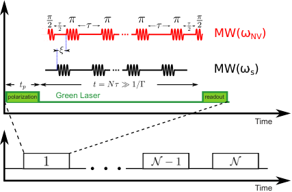
Using two independent microwave sources we apply a train of -pulses first to the qubit and subsequently a Carr-Purcell-Meiboom-Gill (CPMG) pulse sequence [22, 23] to the NV-center, see Fig. 2. As the qubit is pulsed it will drive the FM at the frequency of the pulse sequence , being the time between the application of two subsequent -pulses. When is close to the ferromagnetic resonance (FMR) frequency, , the response of the FM becomes large and one obtains a large amplification of the magnetic field felt by the NV-center. The pulses are applied to the qubit only until the FM reaches steady state precession. We also allow for a possible time offset, , between the pulse sequences applied to the qubit and the NV-center, see Fig. 2. Here, may be chosen to compensate for the phase difference between the driving of the qubit and the response of the FM, thus maximizing the amplification. Since the microwave field applied to the qubit is a sequence of -pulses, the polarization is simply , where may take the values according to the pulse sequence. It is worth noting that even though we excite the FMR with the inhomogeneous dipolar field of the qubit, only the lowest Kittel mode is excited since for small FM higher modes are separated by an energy gap that exceeds the perturbation amplitude. Therefore the macrospin approximation used in Eq. (1) is justified.

III Amplification
We now consider our particular scenario wherein a FM is introduced at a distance from the qubit and from the NV-center (Fig. 1). In this case, both the accumulated phase and the dephasing of the NV-center are modified by the presence of the FM. Because our amplification crucially depends on the series of pulses applied to the NV-center and qubit, here we detail the pulse sequence, see Fig. 2. First we apply, on the qubit only, -pulses separated by a time interval , for a total time of —during this time the FM reaches steady state precession. Next we initialize the NV-center in state , which takes time . Then, a pulse is applied to the NV-center allowing it to accumulate the phase from the FM tilt stray field. Consequently, a series of -pulses are applied to both the NV-center and qubit for a total interrogation time . Finally we apply to the NV-center a -pulse which is, in general, along an axis in the plane orthogonal to the NV-center axis and different from the first -pulse by an angle . The probability that the NV-center occupies the state or after the pulse sequence is now a function of the accumulated phase
| (2) |
Here, are the two possible outcomes when the state of the NV-center is measured, is the dephasing of the NV-center, and is the expectation value in the Gibbs state. Because the accumulated phase itself depends on the value of the qubit magnetic moment , a measurement of the NV-center is a measurement of . The variance in the measured value of the NV-center can be reduced by repeating the measurement times (Fig. 2). Because typically and therefore , the total measurement time is marginally prolonged by the initial pulse sequence that initialized the tilt of the FM.
Given Eq. (2), one may show quite generally that, in the relevant experimental limit when , the AC sensitivity of the NV-magnetometer is given by
| (3) |
which defines the minimum detectable magnetic field for a given total measurement time. Here, , the measurement contrast, is the relative difference in detected signal depending on spin-projection of the NV-center spin, and is the detection efficiency which takes into account that many measurements have to be performed in order to detect a photon. [24] A detailed derivation of Eq. (3) can be found in Appendix B. The sensitivity is small (i.e., ‘good’) when the NV-center dephasing is small while the accumulated phase is large. When the qubit is directly coupled to the NV-center (unamplified) the dephasing time of the NV-center is given by s [25, 26] so that .
As we show in Appendix D, given the pulse sequence described above, when and , where is the linewidth of the ferromagnet, there is a resonant response of the FM while the NV-center picks up non-resonant noise. As such, the ratio of the dephasing to the accumulated phase of the qubit is minimized thereby optimizing the sensitivity. We henceforth take in the remainder of the text.
The accumulated phase is formally
| (4) |
where is the gyromagnetic ratio of the NV. where [] is a complex combination of the magnetic stray-field for the FM polarization along the and axes at the position of the NV-center (qubit), (), and is the NV-center polarization axis. Within the linear response regime and using the pulse sequence described above and optimally choosing , the expression for the phase accumulated by the NV-center when , 33 3 The Fourier transform of the CPMG pulse sequence has peaks at frequencies for , is
| (5) |
where is the gyromagnetic ratio of the FM. is defined such that the resonantly driven FM undergoes half-periods between consecutive -pulses applied to the NV-center. In the optimal case we have so that is half the period of precession of the ferromagnet. The details of the derivation of Eq. 5 can by found in Appendix D. It is readily observed from the above equation that which is proportional to the AC magnetic susceptibility of the FM on resonance; thus we indeed obtain a resonant response as anticipated. Even though the phase accumulated due to the FM tilt is large, the angle of the FM tilt is small ( if the qubit is a nuclear spin) because . Therefore, we can neglect the effects of the backaction of the FM tilt on the qubit, because the stray field modulation induced by the tilt is small compared to the qubit Rabi amplitude and far detuned from the qubit Larmor precession frequency (i.e. ). Thus, the qubit is polarized along the FM stray field ; the scalar product is nonzero only if the stray field of the FM tilt has a component along at the position of the qubit. We address the optimal geometry and position of the qubit relative to the FM in Sec. III.2.
The relevant dephasing is the maximum of the inherent dephasing of the NV-center, , and the dephasing due to the coupling to the FM, [22]
| (6) |
Here is the autocorrelation function of the FM noise. Again taking , we show in Appendix D.2 that
| (7) |
Because , the NV-center indeed accumulates non-resonant noise.
After substituting and from Eq. (5) and Eq. (7) into Eq. (3) and performing the optimization over the interrogation time in Eq. (3), we find the ratio of the unamplified to the amplified sensitivity
| (8) | ||||
where is the dipolar field of the qubit at the position of the NV-center in the unamplified case and is the NV-center decoherence time when the FM is not present; these quantities define the unamplified sensitivity. The biggest amplification is obtained when one half-period of the FM oscillation occurs over the timescale , i.e., . In practice, experimental limitations, such as limitations to the qubit Rabi frequency, bound and therefore from below. Thus, in order to achieve the resonance, one has to use (at the expense of sensitivity) or to tune the FMR frequency as described in the following subsection.
III.1 Tuning the FMR frequency
It has been demonstrated experimentally [28] that the electron spin of NV-centers can be coherently driven at GHz frequency. For a proton spin, however, the same drive would yield Rabi oscillations in the MHz range. Because typical FMR frequencies are in GHz range, needs to be reduced in order for the proton Rabi frequency to be on resonance with the FMR.
One way to decrease is to apply an external magnetic field antiparallel to , [29] whereby there is a metastable state when , with the FM (crystalline and shape) anisotropy field. In Fig. 3, we plot the energy of the FM as a function of angle of the magnetization with respect to the easy axis, according to Eq. (1). It is straightforward to show that the FMR frequency in the metastable state is . On the other hand, the ferromagnet will relax to the thermal state on a timescale given by the Arrhenius law , where is the attempt time. We can insure that the FM is initialized in the metastable state by first measuring the direction of the magnetization, applying an external magnetic field antiparallel to and checking subsequently that the FM magnetization direction is unchanged, which can be done under a nanosecond. [30, 31] In order for the ferromagnet to remain in the metastable state while the measurement is being performed, we require . Indeed, the total measurement time should be larger than the FMR initialization time , and smaller than Arrhenius’ timescale , see Fig. 2. Thus, if we want to tune to a certain value and work at room temperature, the Arrhenius law suggests that the FM volume must satisfy
| (9) |
in order for the metastable state lifetime to be bigger than the measurement time. Here is the Gilbert damping of the FM. Substituting Eq. (9) for the minimal volume into Eq. (8) we obtain
| (10) |
Compared to the amplification formula in Eq. (8), the above equation is independent of the FMR frequency and the FM volume . Thus, irrespective of the choice of the frequency we work at, the same value for the amplification is obtained. Furthermore, the only dependence on the volume is incorporated in the stray fields but, as shown in Sec. III.2, this dependence is weak in the limit . The volume in Eq. (9) is implicitly bounded from above in order to remain in the regime where the macrospin approximation is valid. As detailed in Sec. III.3, FMs with volumes corresponding to MHz resonance at room temperature are well-described by a single classical spin.
III.2 FM geometry and demagnetizing fields
In the absence of an external magnetic field, the qubit aligns along the stray field direction of the FM, while the FM spins are aligned along the easy axis, according to Eq. (1). Because , the FM tilt induced by the qubit is negligible. Therefore, the qubit will align along the direction of the stray field produced by the FM. However, for most geometries of the FM and positions of the qubit, , and therefore the amplification . In the following discussion, we consider our ferromagnet to be a cube of side , but our conclusions can be straightforwardly generalized to other geometries. To gain insight into the direction and strength of the stray field, we use the well-known analogy between the stray field of a homogeneously magnetized body and an electric field produced by surface charges, [32] see Fig. 4. Specifically, we may consider the surfaces of the cube to have charge density , where is the vector normal to the surface of the cube. Therefore, when the position of the qubit is very close to the center of the FM surface which is perpendicular to the polarization direction (here assumed along -axis), points along the -axis, see Fig. 4. Similarly, and are almost aligned with the and axes close to the surface, respectively. Therefore, in these positions, . However, this is not true near the edges of the ferromagnet. Therefore, in order to obtain a strong amplification, one needs, first, a ferromagnet with edges and, second, to position the qubit close to the edges. One may show analytically and numerically (see Fig. 5) that close to the edges is about an order of magnitude bigger than close to the face center and that it has local maxima close to the cube’s corners.

In evaluating , we assume that the FM is homogeneously magnetized as, in cubic geometry, one can find an analytical formula for the stray field in this case, see Appendix E. However, it is important to note that due to demagnetizing fields (arising from dipole-dipole interactions in the FM), the FM ground-state is not homogeneous but rather “flowerlike”. [33] Specifically, the canting of the spins close to the edges is more pronounced, [32] which modifies the FM stray field close to the edges. To account for the effects of the demagnetizing fields, we perform micromagnetic simulations in OOMMF. 44 4 The code is available at http://math.nist.gov/oommf In Fig. 5 we plot in the -plane that is nm above the upper face of the cube. We find that the inclusion of demagnetizing fields changes our value of by only as compared to the uniformly magnetized cube. Therefore, we expect the analytical expression for the stray field to be valid for our choice of parameters.

Because the amplification depends on and only through the stray fields, here we detail this dependence and show that our scheme is robust against small variations of and . The stray fields above the face-center of the cube are equivalent to the electric field of an infinitely charged plane. Therefore, when and the NV-center is near the center of the cube face, the amplification is independent of . On the other hand, the stray field close to the cube edge in comparison to is equivalent to the electric field of a set of infinite line charges. Therefore, there is a logarithmic dependence of the stray field on the distance to the edge, , of the cube in units of so that the amplification is weakly dependent on .
Typical values of the stray fields at the position of the qubit and NV-center in the limit for YIG are on the order of a few hundreds of Gauss. While the presence of a magnetic field perpendicular to the NV-center axis can significantly limit the read-out fidelity of the NV-center, it was found that the fields up to mT can be tolerated. [35] Therefore, we conclude that one can either place the NV-center at distances where the stray field does not exceed mT or care must be taken that the stray field is mostly aligned along the NV-center axis.
III.3 Estimates
In this section we give estimates for the amplification for two cases: detecting a nuclear spin and an electron spin. For all the estimates provided herein, we assume room temperature and that the FM material is YIG, so that , T, and mT. [36] For simplicity but without loss of generality, we assume that the FM has the shape of a cube for the estimates given below. For a cube and in the macrospin approximation there is no contribution from shape anisotropy. Because in typical experiments [10] nm and nm, we take these values for our estimates below.
For detecting a single nuclear spin, we need to tune the FMR to the MHz range and thus, according to Eq. (9), the optimal FM volume corresponds to a cube side nm. In this regime , and thus the amplified sensitivity only weakly depends on the particular choice of and . Taking s, which is the best case scenario for the unamplified sensitivity and subsequently worst case for amplification, we obtain . Since state-of-the-art NV-magnetometers can resolve clusters of about 300 nuclear spins at a distance of nm, [37, 38, 9, 11] the amplification by three orders of magnitude obtained herein suffices for resolving a single nuclear spin at a distance of nm from the surface.
We note that the volume considered in our estimate corresponds to ns [see Eq. (7)], which is also the value of the optimal interrogation time, and therefore even when the “bare” 10 ns (i.e., the time in the absence of the FM), the decoherence time of the NV-center is limited by the FM noise. Thus, because the signal amplification in our scheme far exceeds the effect of the additional decoherence it induces, even shallow NV-centers [26, 25] with relatively short decoherence time can be used and significantly outperform unamplified long-lived NV-centers.
To amplify the signal from a single electron spin, there is no need to tune down the FMR frequency since the electron spin can be driven at GHz frequencies. Thus, one can use the stable state of the FM and therefore there is no restriction on the minimum FM volume. With the same distances and as in the nuclear spin case and for nm, corresponding to the volume of maximum amplification, we obtain . In order to obtain this estimate, we used the fact that the relaxation time of the electron spin is typically shorter than the NV-center time and that the NV-center interrogation time cannot be longer than the relaxation time of the electron spin. [10] Thus, in Eq. (10) we use a typical electron spin relaxation time ns in place of . [10] If we choose nm and nm, we obtain an amplification as big as for nm.
IV Conclusions
We have proposed and analyzed, both analytically and numerically, a modification of a standard NV-magnetometry setup that yields a significant improvement of NV-magnetometer sensitivity by up to four orders of magnitude. Our scheme is based on a ferromagnetic particle, placed in close proximity to a sensing NV-center spin. The qubit spin to be detected is then used to resonantly drive the large macrospin of the FM giving rise to a strong, amplified stray field acting on the NV-magnetometer. Compared to the existing schemes that use the quantum nature of an intermediate spin for improving sensitivity, [18] we stress that our scheme is fully classical and thus should be easily realizable at room temperature—all the ingredients of our scheme are already demonstrated in separate experiments. [28, 10, 39, 40]
An alternative setup to achieve resonance between the qubit and FM is to place the NV-center and the FM on a cantilever [41] with resonance frequency in the GHz range. By driving the cantilever, we alleviate the necessity of driving the qubit at FMR frequency as the qubit field is modulated by the oscillations of the cantilever. Since the dipolar field of the qubit decays rapidly with distance, the modulation of the qubit field achieved in this scheme is almost as big as when the qubit is driven via a microwave field (the previously described scheme for which the amplification estimates are given). Therefore, we conclude that the estimates for the sensitivity amplification given in Sec. III.3 still hold in that case.
The magnetometric scheme including a ferromagnetic particle proposed here is a step forward to a more accurate magnetic field measurement. In particular, it enables the detection of a single nuclear spin at distances that are noninvasive to the system under study. Therefore, the proposed room temperature amplification method opens up new venues for future analyses of previously inaccessible biological and chemical systems.
V Acknowledgments
We would like to thank H. Fanghor for sharing his expertise about micromagnetic simulations. This work was supported by the SNF, NCCR QSIT, IARPA, DARPA QuASAR programs and the MURI QuISM. F. L. P. is grateful for support from the Alexander von Humboldt foundation.
Appendix A Cramer-Rao Bound
For the sake of completeness, we review here the proof of the Cramer-Rao bound,
| (11) |
that we use to derive the sensitivity expression (3) in the main text.
The Fisher information of the parameter estimator is given by
| (12) |
The Cramer-Rao bound follows from the trivial identity
| (13) |
where . Taking the derivative of this identity with respect to and using the fact that the estimator does not depend explicitly on , we obtain
Appendix B Sensitivity of an NV-center
The variance of any estimator of the unknown parameter satisfies the Cramer-Rao inequality Eq. (11). Using the probability distribution from Eq. (2) we obtain
| (15) |
Thus, a bigger Fisher information leads to a more accurate value of the estimator .
For DC magnetometry we typically have and , where GHz is the zero-field splitting of the NV-center and is typically on the order of a few microseconds. The field we want to measure is , with the distance between the qubit and the NV-center. Consider the scenario which is valid for DC magnetometry. In such a situation, one may choose an interrogation time maximizing and minimizing in Eq. (15). This is independent of the angle which we set to zero without loss of generality. Thus instead of maximizing the Fisher information from Eq. (15), we need only to maximize its envelope function,
| (16) |
Repeating the measurement times ( is the initialization time) reduces the variance by a factor . The Cramer-Rao bound (11) then leads to . The minimal value of the magnetic moment (that can be resolved within measurement time and interrogation time ) is determined by the one for which the mean value is equal to its standard deviation,
| (17) |
Assuming , we finally obtain the sensitivity
| (18) |
As mentioned in the main text, is the measurement contrast and is the detection efficiency; [24] these quantities take into account that the measurement has to be performed many times in order to detect a photon.
The situation for AC magnetometry is different; here while we still have . (Note that the constant of proportionality depends on the specific pulse sequence applied.) In typical situations, the AC magnetic field is small and . In such scenario, and for vanishing angle , the accumulated phase will never reach a value of and one needs to maximize the Fisher information (15), not only its envelope. In this limit, we obtain a very different expression for the sensitivity, and, in particular, the expression is in units of “magnetic moment” (see Appendix C). Fortunately, such result can be improved: one may take a nonzero value of the angle such that the expression within the interrogation time. In this case, the amplified sensitivity takes the form (18), improving the sensitivity.
Appendix C AC sensitivity for
The goal of this appendix is to derive the expression for the AC sensitivity when the angle between the two -pulses, applied at the beginning and at the end of the sequence, is zero. This calculation is presented for the sake of completeness, however, this is not the expression we use to derive our amplified sensitivity. As mentioned in the main text, for AC magnetometry we have
| (19) | ||||
| (20) |
where the constant of proportionality depends on the specific pulse sequence applied. It is important to note that here only the AC field component that matches the frequency of the pulse sequence contributes (i.e., there is no contribution from ). When the magnitude of the AC driving field is small, we are in the limit of . As noted above, in this regime the accumulated phase will not reach the value of and thus the full Fisher information needs to be maximized. Namely, we maximize
| (21) |
Therefore,
| (22) |
In contrast to the result obtained in Ref. 18 [which is similar to the one obtained in Eq. (16)], the Fisher information in Eq. (22) depends on the estimation parameter . The minimal value of the magnetic moment (that can be resolved within measurement time and interrogation time ) is again determined as the one for which the mean value is equal to its standard deviation, Eq. (17). Therefore, using the fact that depends linearly on and that for typical interrogation time , we find an approximate solution to Eq. (17). Minimizing over the interrogation time, we obtain
| (23) | ||||
Now, if we remove the dependence on the total measurement time from the above expression, we obtain the quantity that describes the magnetic moment sensitivity in units of “magnetic moment”, i.e.,
| (24) |
Appendix D Calculation of and
The goal of this appendix is to give a detailed derivation of Eqs. (5) and (7) that are central to our work. The former describes the phase accumulated by the NV-magnetometer, while the latter the variance of this accumulated phase.
Within linear response, the accumulated phase is
| (25) |
where () is the time offset between the CPMG pulse sequence applied to the qubit and the NV-center. We have introduced the following notation,
| (26) | ||||
| (27) |
with and . After performing the integral in Eq. (26) and using , , we obtain
| (28) | ||||
| (30) |
Since we want the qubit to perturb the ferromagnet within a narrow frequency window around the FMR (i.e., narrower than the FMR linewidth ), we require that . In this limit, the expression for is significantly simplified
| (31) | ||||
| (32) | ||||
The expression for dephasing can be obtained from [22]
| (33) |
Furthermore,
| (34) |
In the limit ( is the anisotropy field) one obtains the following expression for the fluctuations of the ferromagnet,
| (35) |
Combining equations (33-35) we finally obtain
| (36) |
D.1 On-resonance case
The Fourier transform of the CPMG sequence depicted in Fig. 2 has peaks at frequencies . Thus we have a resonant behavior whenever this frequency matches . Assuming and leads to the following expression for , namely
| (37) |
where . Assuming , we can neglect the second term in the bracket in Eq. (37) and obtain the expression for the phase accumulated by the NV-center during the interrogation time ,
| (38) |
Next, we choose the time offset (i.e., ) such that in the above equation is maximized
| (39) |
we obtain
| (40) |
Assuming that the optimal interrogation time satisfies , we arrive at the following expression for , namely
| (41) |
The above expression yields the following variance of the phase accumulated by the NV-center
| (42) |
D.2 Pulse sequence applied: a matter of timescales
Here we elucidate the importance of the different duration of the pulse sequences applied to the qubit and the NV-center. We analyze what happens to the amplification when both pulse sequences have the same duration, see Fig. 6. Performing the Fourier transform of Eq. (33), one obtains
| (43) |
Here the subscript refers to the Fourier transform evaluated at frequency . We assume that the filter function is centered around the frequency (on-resonance case) and that it is much narrower than the FMR linewidth, i.e., —this is exactly the opposite limit from the one assumed to arrive at Eq. (7). The accumulated phase is given in Eq. (5), and thus the magnetic moment sensitivity in this case reads
| (44) |
where . The above expression yields almost no amplification, since we do not only excite the FM resonantly but also the NV-center picks up the resonant noise. If we rewrite Eq. (7) in the form , we can understand that the decoherence times in the two considered limits differ from each other by many orders of magnitude, namely
| (45) |

Appendix E Stray field from a uniformly magnetized cuboid
In this section we review the analytical formulas giving the stray field of a uniformly magnetized cuboid of side lengths , , and , see Fig. 4. As mentioned in the main text, the magnetic field at a point outside of the cuboid can be calculated from the expression for the electric field originating from charges uniformly distributed on the surfaces of the cuboid perpendicular to the magnetization, [42, 43] see Fig. 4. For the sake of simplicity, we assume that the magnetization direction points either along , , or . The expression for the stray field is then
| (46) |
for . Here, and are the directions perpendicular to , i.e., , , and , and .
The integrals in Eq. (46) can be evaluated analytically. [42, 43] When the cuboid is magnetized along , one obtains
| (47) | |||
| (48) | |||
| (49) |
Here
| (51) |
The analytical expressions for are found similarly.
For the sake of illustration, we plot in Fig. 7 the three components of as function of and for a cube of size at a distance of above the upper face.
References
- [1] R. Ernst, G. Bodenhausen, and A. Wokaun, Nuclear Magnetic Resonance in One and Two Dimensions (Oxford Univ. Press, Oxford, 1987).
- [2] P. Hemmer, Science 339, 529 (2013).
- [3] J. A. Sidles, Applied Physics Letters 58, 2854 (1991).
- [4] E. Ramsden, Hall-Effect Sensors, Second Edition: Theory and Application, 2nd ed. (Newnes, Amsterdam ; Boston, 2006).
- [5] M. E. Huber, N. C. Koshnick, H. Bluhm, L. J. Archuleta, T. Azua, P. G. Björnsson, B. W. Gardner, S. T. Halloran, E. A. Lucero, and K. A. Moler, Rev. Sci. Instrum. 79 (2008).
- [6] C. L. Degen, M. Poggio, H. J. Mamin, C. T. Rettner, and D. Rugar, Proc. Natl Acad. Sci. USA 106, 1313 (2009).
- [7] M. Poggio and C. L. Degen, Nanotechnology 21, 342001 (2010).
- [8] P. Peddibhotla, F. Xue, H. I. T. Hauge, S. Assali, E. P. A. M. Bakkers, and M. Poggio, Nat Phys 9, 631 (2013).
- [9] H. J. Mamin, M. Kim, M. H. Sherwood, C. T. Rettner, K. Ohno, D. D. Awschalom, and D. Rugar, Science 339, 557 (2013).
- [10] M. S. Grinolds, M. Warner, K. D. Greve, Y. Dovzhenko, L. Thiel, R. L. Walsworth, S. Hong, P. Maletinsky, and A. Yacoby, Nat. Nano. 9, 279 (2014).
- [11] T. Staudacher, F. Shi, S. Pezzagna, J. Meijer, J. Du, C. A. Meriles, F. Reinhard, and J. Wrachtrup, Science 339, 561 (2013).
- [12] L. Rondin, J. P. Tetienne, T. Hingant, J. F. Roch, P. Maletinsky, and V. Jacques, Rep. Prog. Phys. 77, 056503 (2014).
- [13] G. Waldherr, J. Beck, P. Neumann, R. S. Said, M. Nitsche, M. L. Markham, D. J. Twitchen, J. Twamley, F. Jelezko, and J. Wrachtrup, Nat Nano 7, 105 (2012).
- [14] L. C. Bassett, F. J. Heremans, D. J. Christle, C. G. Yale, G. Burkard, B. B. Buckley, and D. D. Awschalom, Science (2014).
- [15] P. Maletinsky, S. Hong, M. S. Grinolds, B. Hausmann, M. D. Lukin, R. L. Walsworth, M. Loncar, and A. Yacoby, Nat. Nano 7, 320 (2012).
- [16] We emphasize that we denote the target magnetic moment by ’qubit’ solely for the purpose of convenience in nomenclature and that our scheme does not rely on the quantum nature of the magnetic moment we aim to measure.
- [17] M. Loretz, S. Pezzagna, J. Meijer, and C. L. Degen, App. Phys. Lett. 104 (2014).
- [18] M. Schaffry, E. M. Gauger, J. J. L. Morton, and S. C. Benjamin, Phys. Rev. Lett. 107, 207210 (2011).
- [19] Instead of performing the qubit control resonantly, one can make use of ‘adiabatic passage’ [44] wherein triangular pulses are applied in lieu of square pulses. In such a setup, knowledge of the exact value of the qubit Zeeman splitting, and therefore the FM stray field, is not needed.
- [20] E. C. Stoner and E. P. Wohlfarth, Phil. Trans. R. Soc. A 240, 599 (1948).
- [21] L. Trifunovic, F. L. Pedrocchi, and D. Loss, Phys. Rev. X 3, 041023 (2013).
- [22] L. Cywinski, R. M. Lutchyn, C. P. Nave, and S. Das Sarma, Phys. Rev. B 77, 174509 (2008).
- [23] G. de Lange, Z. H. Wang, D. Riste, V. V. Dobrovitski, and R. Hanson, Science 330, 60 (2010).
- [24] V. M. Acosta, E. Bauch, M. P. Ledbetter, C. Santori, K.-M. C. Fu, P. E. Barclay, R. G. Beausoleil, H. Linget, J. F. Roch, F. Treussart, S. Chemerisov, W. Gawlik, and D. Budker, Phys. Rev. B 80, 115202 (2009).
- [25] K. Ohno, F. Joseph Heremans, L. C. Bassett, B. A. Myers, D. M. Toyli, A. C. Bleszynski Jayich, C. J. Palmstrom, and D. D. Awschalom, App. Phys. Lett. 101, 082413 (2012).
- [26] B. A. Myers, A. Das, M. C. Dartiailh, K. Ohno, D. Awschalom, D., and C. Bleszynski-Jayich, A., Phys. Rev. Lett. 113, 027602 (2014).
- [27] The Fourier transform of the CPMG pulse sequence has peaks at frequencies .
- [28] G. D. Fuchs, V. V. Dobrovitski, D. M. Toyli, F. J. Heremans, and D. D. Awschalom, Science 326, 1520 (2009).
- [29] D. O. Smith, J. App. Phys. 29, 264 (1958).
- [30] M. Julliere, Phys. Lett. A 54, 225 (1975).
- [31] K.-J. Lee, A. Deac, O. Redon, J.-P. Nozieres, and B. Dieny, Nat. Mater 3, 877 (2004).
- [32] V. N. Samofalov, D. P. Belozorov, and A. G. Ravlik, Physics-Uspekhi 56, 269 (2013).
- [33] A. Aharoni, Introduction to the Theory of Ferromagnetism, 2nd ed. (Oxford University Press, Oxford ; New York, 2001).
- [34] The code is available at http://math.nist.gov/oommf.
- [35] J.-P. Tetienne, L. Rondin, P. Spinicelli, M. Chipaux, T. Debuisschert, J.-F. Roch, and V. Jacques, New J. of Phys. 14, 103033 (2012).
- [36] N. L. Schryer and L. R. Walker, J. App. Phys. 45, 5406 (1974).
- [37] G. Balasubramanian, I. Y. Chan, R. Kolesov, M. Al-Hmoud, J. Tisler, C. Shin, C. Kim, A. Wojcik, P. R. Hemmer, A. Krueger, T. Hanke, A. Leitenstorfer, R. Bratschitsch, F. Jelezko, and J. Wrachtrup, Nature 455, 648 (2008).
- [38] J. R. Maze, P. L. Stanwix, J. S. Hodges, S. Hong, J. M. Taylor, P. Cappellaro, L. Jiang, M. V. G. Dutt, E. Togan, A. S. Zibrov, A. Yacoby, R. L. Walsworth, and M. D. Lukin, Nature 455, 644 (2008).
- [39] E. Schäfer-Nolte, L. Schlipf, M. Ternes, F. Reinhard, K. Kern, and J. Wrachtrup, ArXiv e-prints (2014), arXiv:1406.0362 .
- [40] C. S. Wolfe, V. P. Bhallamudi, H. L. Wang, C. H. Du, S. Manuilov, R. M. Teeling-Smith, A. J. Berger, R. Adur, F. Y. Yang, and P. C. Hammel, Phys. Rev. B 89, 180406 (2014).
- [41] J. Teissier, A. Barfuss, P. Appel, E. Neu, and P. Maletinsky, Phys. Rev. Lett. 113, 020503 (2014).
- [42] J. Norpoth, S. Dreyer, and C. Jooss, J. Phys. D: Appl. Phys. 41, 025001 (2008).
- [43] R. Engel-Herbert and T. Hesjedal, J. Appl. Phys. 97, 074504 (2005).
- [44] G. D. Fuchs, G. Burkard, P. V. Klimov, and D. D. Awschalom, Nat. Phys 7, 789 (2011).