Dirac open quantum system dynamics: formulations and simulations
Abstract
We present an open system interaction formalism for the Dirac equation. Overcoming a complexity bottleneck of alternative formulations, our framework enables efficient numerical simulations (utilizing a typical desktop) of relativistic dynamics within the von Neumann density matrix and Wigner phase space descriptions. Employing these instruments, we gain important insights into the effect of quantum dephasing for relativistic systems in many branches of physics. In particular, the conditions for robustness of Majorana spinors against dephasing are established. Using the Klein paradox and tunneling as examples, we show that quantum dephasing does not suppress negative energy particle generation. Hence, the Klein dynamics is also robust to dephasing.
pacs
03.65.Pm, 05.60.Gg, 05.20.Dd, 52.65.Ff, 03.50.KkI Introduction.
The Dirac equation is a cornerstone of relativistic quantum mechanics [1]. It was originally developed to describe spin charged particles playing an essential role in the field of high energy physics [2, 3, 4]. Recently, there is resurging interest in the Dirac equation because it was found to be an effective dynamical model of unexpectedly diverse phenomena occurring in high-intensity lasers [5], solid state [6, 7, 8, 9], optics [10, 11], cold atoms [12, 13], trapped ions [14, 15], circuit QED [16], and the chemistry of heavy elements [17, 18]. However, there is a need to go beyond coherent dynamics offered by the Dirac equation alone in order to model the effects of imperfections, noise, and interaction with a thermal bath [19]. To construct such models, we will first review how these effects are described without relativistic considerations [20].
In the non-relativistic regime, the Schrödinger equation describes a quantum systems isolated from the rest of the universe. This is a good approximation for certain conditions. For example, an atom in a dilute gas can be considered to be a closed system if the time scale of the dynamics is much faster than the mean collision time. If we would like to include collisions in the picture, we need to keep track of the quantum phases of each atom in the gas. This is unfeasible. This type of dynamics motivated development of the theory of open quantum systems [21], where a single particle picture is retained albeit with more general dynamical equations. There are two methods to introduce interactions with an environment: (i) the Schrödinger equation with an additional stochastic force, or (ii) the conceptually different density matrix formalism [20]. In the latter, a state of an open quantum system is represented by a self-adjoint density operator with non-negative eigenvalues summing up to one. The master equation, governing evolution of , reads
| (1) |
where is the quantum Hamiltonian and the dissipator encodes the interaction with an environment. The von Neumann equation [20] describing unitary evolution is recovered by ignoring the dissipator. When , Eq. (1) generally does not preserve the von Neumann entropy , which measures the amount of information stored in a quantum system. We note that effective elimination of is a fundamental challenge in order to develop many quantum technologies [22, 23].
The non-relativistic theory of open quantum systems provided profound insights into some fundamental questions of physics such as the emergence of the classical world from the quantum one [24, 25, 26, 27, 28, 29, 30], measurement theory [24, 31, 32, 33], quantum chaos [34, 27, 30] and synchrotron radiation [35, 36, 37].
To study the quantum-to-classical transition, it is instrumental to put both mechanics on the same mathematical footing [38, 39, 40, 25, 28, 24, 31, 41, 42, 43, 44, 45]. This is achieved by the Wigner quasi-probability distribution [46], which is a phase-space representation of the density operator . Note that the Wigner function serves as a basis for a self-consistent phase space representation of quantum mechanics [42, 47], which is equivalent to the density matrix formalism.
Previous attempts to construct the relativistic theory of open quantum system relied on the relativistic extension of the Wigner function without introducing the corresponding density matrix formalism. In Sec. II, we will first present the manifestly covariant density matrix formalism for a Dirac particle and then construct the Wigner representation. The development of the relativistic Wigner function was motivated by applications in quantum plasma dynamics and relativistic statistical mechanics [3]. The manifestly covariant relativistic Wigner formalism for the Dirac equation was put forth in Refs. [48, 49, 2, 50] (see Ref. [3] for a comprehensive review). In addition, exact solutions for physically relevant systems were reported in Refs. [51, 52]. The following conceptual difference between the non-relativistic and relativistic Wigner functions was elucidated in Ref. [53]: In non-relativistic dynamics, Hudson’s theorem states that the Wigner function for a pure state is positive if and only if the underlying wave function is a Gaussian [54]. In other cases, the Wigner function contains negative values. However, this statement does not carry over to the relativistic regime. In particular, there are many physically meaningful spinors whose Wigner function is positive [53]. Note that the Wigner function’s negativity is an important resource in quantum information theory [55, 56].
The limit of the non-relativistic Wigner function is non-singular and recovers classical mechanics. The same limiting property is expected from the relativistic extension. However, the manifest covariance of the relativistic Wigner function needed to be broken in order to perform the limit [57, 50, 58]. From a different perspective, the covariant classical limit was obtained in Refs. [59, 41]. In Appendix B of the current work, we provide a simpler manifestly-covariant derivation of the classical limit. Contrary to the previous work, our derivation recovers two decoupled classical equations of motion: one governing the dynamics of positive energy particles and the other describing negative energy particles (i.e., antiparticles). This classical limit of the Dirac equation is an example of classical Nambu dynamics [60].
An alternative quantum field theoretic formulation of the Wigner function for Dirac fermions has also been put forth [57, 61, 62, 63, 64, 65, 66].
As mentioned before, the current interest in the Dirac equation goes far beyond relativistic physics. These new opportunities come along with new challenges. It is the aim of the current Article to overcome some of those problems by furnishing a new formulation of traditional (i.e., closed system) relativistic dynamics enabling efficient numerical simulations as well as physically consistent inclusion of open system interactions. We believe that the developed formalism and numerical methods will influence the following fields:
- 1.
Understanding the role of the environment for the classical world emergence. In particular, we elucidate the influence of decoherence (i.e., loss of quantum phase coherence) on relativistic dynamics in Secs. VI and VII, where Klein tunneling [7] and the associated paradox are analyzed along with the Majorana fermion dynamics.
- 2.
Development of the quantum relativistic theory of energy dissipation. Based on existing models of non-relativistic quantum friction [67, 68], we expect a relativistic model of energy damping to obey: (i) the mass-shell constraint, (ii) translational invariance (in particular, the dynamics should not depend on the choice of the origin), (iii) equilibration (the model should reach a steady state at long time propagation. In particular, the final energy at should be bounded thereby preventing runaway population of the negative energy continuum), (iv) thermalization (i.e., the achieved steady state should represent thermal equilibrium), (v) relativistic extension of Ehrenfest theorems (i.e., see the dynamical constraints for expectation values encompassing energy drain in Ref. [68]). Some preliminary steps towards the desired relativistic model are reported in Ref. [69].
- 3.
Modeling environmental effects in Dirac materials such as topological insulators [8, 70, 71], Weyl semimetals [72, 73], and graphene [6]. In these cases, open system dynamics models sample impurities and imperfections as well as external noise. Recently, the Dirac equation with an additional stochastic force was utilized for this purpose [19]. To the best of our knowledge, a more general master equation formalism is yet to be explored.
- 4.
Understanding robustness of a Majorana particle, which is defined as being its own antiparticle. Experimental implementation of solid-state analogues of Majorana fermions [74, 75, 76] opens up possibilities to study the physics of these unusual states. In particular, Majorana bound states are well suited components of topological quantum computers [77]. Due to its topological nature, Majorana states are expected to be robust against perturbations and imperfections [78]. Dissipative dynamics modeled within a Lindblad master equation confirmed a significant degree of robustness in a specific optical lattice [79]. However, the robustness is not universal [80] and there is a need for enhancement (e.g., employing error correction techniques [81]). Note that Majorana states studied in condensed matter physics [74, 75, 76], do not strictly coincide with the authentic Majorana spinors [82], albeit sharing common features. In the present paper, we consider original Dirac Majorana spinors [82]. In Sec. VI, we demonstrate that a single-particle Majorana spinor exhibits robustness even for strong couplings to the dephasing environment, which otherwise quickly washes out interferences for particle-particle superpositions (aka, Schrödinger cat states). Moreover, this phenomenon has an intuitive explanation in the phase-space representation, where quantum dephasing turned out to be equivalent to Gaussian filtering over the momentum axis (detailed explanation in Secs. IV and V). The applicability of this insight to condensed matter systems should be a subject of further studies.
- 5.
Development of manifestly covariant quantum open system interaction. Coupling a Dirac particle to the environment generally introduces a preferred frame of reference, thereby breaking the Lorentz invariance. However, coupling to the vacuum, causing spontaneous emission, Lamb shift etc. [83], and radiation reaction [84, 85], needs to be manifestly covariant because the vacuum has no preferred frame of reference. Solid state physics holds a promise to implement many exotic quantum effects experimentally not yet verified [86], e.g., the Unruh effect and Hawking radiation. Solid state dynamics naturally includes the interaction with the environment, thus the need to include open system interaction into the dynamics of interest. A relativistic quantum theory of measurements also requires development of manifestly covariant master equations. Currently, approaches based on axiomatics [87], stochastic Dirac and Lindblad master equations [88] are explored. Nevertheless, the proposed equations are computationally unfeasible at present. In the current work, we lay the ground for a computationally efficient technique by introducing a manifestly covariant von Neumann equation (see Sec. II) based on Refs. [48, 49, 2, 50, 3].
This paper is organized in seven sections and two appendices. Section II provides the general mathematical formalism including the manifestly relativistic covariant von Neumann equation. Section III is concerned with the relativistic Wigner function and related representations. Section IV introduces open system interactions by considering a model of dephasing, environmental interaction leading to the loss of quantum phase. Numerical algorithms are developed in Sec. V and illustrated for the dynamics of Majorana spinors and the Klein paradox in Secs. VI and VII, respectively. The final section VIII provides the conclusions. Appendix A treats the concept of relativistic covariance, and Appendix B elaborates the classical limit () of the Dirac equation in manifestly covariant fashion.
II General Formalism
Note that throughout the paper, and denote different variables; likewise, and denote different operators. In addition, Greek characters (e.g., , ), used as indices for Minkowski vectors, are assumed to run from to ; while, Latin indices (e.g., , ) run from to . The Minkowski metric is a diagonal matrix . This implies that and .
The manifestly covariant Dirac equation reads
| (2) |
where the Dirac generator and the commutation relations are defined as
| (3) | ||||
| (4) |
Note that the negative sign in the right hand side of Eq. (4) occurs due to the fact
| (5) |
in agreement with non-relativistic dynamics where the momentum is expressed in contravariant components .
From the well established work on relativistic statistical quantum mechanics [48, 49, 2, 50, 3], the manifestly covariant von Neumann equation can be written as
| (6) |
where represents the density state operator acting on the Manifestly Covariant Spinorial Hilbert space (MCS). Equation (6) is the foundation for all the subsequent developments.
Following Ref. [89, 90], we introduce the Manifestly Covariant Hilbert Phase space (MCP) where the algebra of observables consists of [see Eq. (4)] along with the mirror operators obeying
| (7) |
and all the other commutators vanish. In MCP the role of density operator is taken over by the ket state according to
| (8) | ||||
| (9) |
where the arrows indicate the direction of application of the operators and . Thus, the relativistic von Neumann equation (6) reads in MCP as
| (10) |
A summary of the two introduced formulations is given in Table 1.
|
| |||||||
|---|---|---|---|---|---|---|---|---|
| State | ||||||||
| Operators | , | |||||||
| Equation | ||||||||
| of motion | ||||||||
The manifest covariance of Eq. (10) can be relaxed to implicit covariance by separating the time according to the splitting [91]. This means that the underlying relativistic covariance is maintained but it is no longer evident. In the spirit of the scheme we define the Dirac Hamiltonian as
| (11) |
The von-Neumann equation (10) in the Implicit Covariant Hilbert Phase space (ICP) becomes
| (12) | |||
| (13) |
Inspired by the Bopp transformations in the non-relativistic quantum mechanical phase space [92, 93], a representation of the algebra (7) can be constructed in terms of ICP Bopp operators in Table 2,
| ICP operators | Mirror ICP operators | |||||||||||||||||||||||||||
|---|---|---|---|---|---|---|---|---|---|---|---|---|---|---|---|---|---|---|---|---|---|---|---|---|---|---|---|---|
|
|
|
obeying
| (14) | ||||
| (15) |
where all the other commutators vanish, in particular . A graphical illustration of the relation between the time variables and is shown in Fig. 1.
Adding and substracting Eqs. (12) and (13), and utilizing the Bopp operators, we obtain the von-Neumann equation in the ICP space
| (16) | ||||
| (17) | ||||
and can be realized in terms of differential operators as
| (18) | ||||
| (19) |
turning Eqs. (16) and (17) into a system of two differential equations that can be solved by either propagating along while keeping fixed, or moving along with constant. In particular, setting in Eq. (16), we obtain the relativistic von-Neumann equation in the Sliced Covariant Hilbert Phase space (SCP)
| (20) | ||||
It is well known that a Lorentz transformation mixes the space and time degrees of freedom, as recapitulated in Appendix A. In particular, the time-evolution of the state in a different reference frame corresponds to a different slicing in the plane. Therefore, the state propagated by Eq. (20) with does not contain enough information to deduce the observations from a different inertial frame of reference. Nevertheless, Eq. (20) represents a consistent relativistic equation of motion describing dynamics from the particular frame of reference (corresponding to the slice) free of any nonphysical artifacts, e.g., superluminal propagation. A schematic illustration of slicing dynamics at is shown in Fig. 2.

Note that equations of motion containing two time variables also appear in non-relativistic dynamics [94].
Using Table 2, we rewrite Eq. (20) in the Hilbert Spinorial space
| (21) |
Note that this equation resembles Eq. (1) with . In other words, we obtain a straightforward relativistic extension of the density matrix formalism for the Dirac equation. Migdal [95] employed Eq. (21) to describe the effect of multiple scattering on Bremsstrahlung and pair production.
III Relativistic Wigner function
This section is devoted to study specific representations of the von-Neumann equation in the SCP space (20) in order to derive the time-evolution of the relativistic Wigner function.

Following Table 2, there are four representations of interest:
- •
The double configuration space is defined by setting
(22) Hence, the equation of motion (20) becomes
(23) where is defined as the relativistic Blokhintsev function
(24) For pure states, is expressed in terms of the four-column Dirac spinor as
(25) Therefore, is a complex matrix-valued function of two degrees of freedom . The non-relativistic version of the Blokhintsev function was introduced in Refs. [96, 97, 98].
- •
The phase space is defined by
(26) The underlying equation of motion (20) reads
(27) where is the sought after relativistic Wigner function
(28) which can be recovered from the Blokhintsev function through a Fourier transform
(29) Note that only contravariant components are used in Eqs. (28) and (29).
- •
The reciprocal phase space is defined as
(30) The corresponding equation of motion is
(31) where is the relativistic ambiguity function
(32) which is recovered from the Blokhintsev function according to
(33) - •
The double momentum space is introduced as
(34) The corresponding equation of motion is
(35) where
(36) which is related with the Wigner function via
(37) Similarly, we also have
(38)
In summary, all these four functions are connected through Fourier transforms as visualized in the following diagram:
where vertical arrows denote the direct Fourier transforms while horizontal arrows indicate the direct Fourier transforms. A similar diagram can be drawn in terms of the inverse Fourier transforms as
Since the relativistic Wigner function is a complex matrix, its visualization is cumbersome. Nevertheless, most of the information is contained in [53]
| (47) |
In fact, this zero-th component is sufficient to obtain the probability density as
| (48) | ||||
| (49) |
where is the Dirac spinor in the momentum representation, i.e. the Fourier transform of .
IV Open system interactions
Inspired by non-relativistic quantum mechanics [see Eq. (1)], we add a dissipator to the relativistic von Neumann equation (21) to account for open system dynamics
| (50) |
We note that Eq. (50) does not need to comply with relativistic covariance. Nevertheless, this is not a deficiency when dealing with environments such as thermal baths that are already furnished with a preferred frame of reference.
Motivated by the treatment of quantum dephasing in non-relativity [20], we propose to include the following dissipator in Eq. (50)
| (51) |
where is the decoherence coefficient controlling the dephasing intensity and no summation on is implied. In non-relativistic systems this interaction is utilized to describe the loss of coherence due to the interaction with an environment associated with a thermal bath [99, 40, 29, 25]. In addition, a system undergoing continuous measurements in position follows the same dynamics [28, 100]. A model similar to Eq. (51) describes the effect of multiple scattering on Bremsstrahlung and pair production in high energy limit of the incident electron [95].
The dynamical effect of an interaction can be characterized by calculating the time derivative of the expectation value of an observable
| (52) |
Assuming that the equation of motion is of the form
| (53) |
the time derivative of is expressed as follows
| (54) |
where is the adjoint operator of with respect to the Hilbert-Schmidt scalar product.
The particular dephasing dissipator (51) is self-adjoint,
| (55) |
as a result,
| (56) |
This means that the dephasing does not change the Heisenberg equations of motion for position and momentum observables. The open system interaction affects the dynamics of the second order momentum
| (57) |
which in turn leads to a momentum wavepacket broadening. Moreover, considering that the free Dirac Hamiltonian (11) is linear in momentum, we obtain from Eqs. (56) and (54)
| (58) |
In other words, the energy is conserved under the action of the dephasing dissipator (51). This is in stark contrast to non-relativistic dephasing, which is characterized by monotonically increasing energy.
The classical limit of dephasing (51) is diffusion. Relativistic extensions of diffusion face fundamental challenges [101]. For instance, large values of may induce dynamics leading to superluminal propagation, which breaks down the causality of the Dirac equation (see, e.g., Theorem 1.2 of Ref. [102]). The length-scale of diffusion is ; hence, the characteristic speed must be smaller than the speed of light. The shortest time interval for which the single particle picture is valid , i.e., the zitterbewegung time scale. Considering all these arguments, we obtain the constrain: , or equivalently, (where is the reduced Compton wavelength) in order to maintain causal dephasing dynamics.
V Numerical algorithm
Stimulated by the resurgent interest in the Dirac equation, a plethora of propagation methods were recently developed [103, 104, 105, 106, 107, 108]. However, to the best our knowledge Ref. [109] is the only work devoted to propagation of the relativistic von Neumann equation (21), albeit without open system interactions. The purpose of this section is to develop an effective numerical algorithm to propagate the master equation (50) describing quantum dephasing (51). The computational effort with the proposed algorithm scales as the square of the Dirac equation propagation complexity. This algorithmic development enables the relativistic Wigner function simulations, which were previously hindered by the complexity of the underlying integro-differential equations [50, 48].
The evolution governed by Eq. (21)
| (60) |
with is equivalent to
| (61) |
where is an infinitesimal time step.
Considering that the Hamiltonian can be decomposed as
| (62) | ||||
| (63) | ||||
| (64) |
where the mass term contributes to both and . The first order splitting with error is then
| (65) |
which implies a two step propagation
| (66) | ||||
| (67) |
Using Eqs. (8) and (9) we move to SCP
| (68) | ||||
| (69) |
Note that is a complex matrix reflecting the spinor degrees of freedom. The arrows can be eliminated by choosing suitable bases
| (70) | ||||
| (71) | ||||
| (72) | ||||
| (73) |
where and stand for Fourier transforms from the momentum representation to the position representation and vice versa. Considering that the state is a matrix, the Fourier transform is independently applied to each matrix component. From the computational perspective, the fast Fourier transform is employed. Further details about the phase space propagation via the fast Fourier transform can be found in Sec. III of Ref. [90].
Having described the propagation algorithm in SCP , one can apply a similar strategy to the Bopp operators (see Table 2). There are multiple advantages of the latter representation. Importantly, some open system interactions (e.g., the dephasing model explained in detail in Sec. IV) take simpler forms in terms of . The momentum and coordinate grids in are interdependent such that if the discretization step size and the grid amplitude of are specified, then the momentum increment and the amplitude of are fixed and vice versa. However, the momentum and position grids in are independent, thus allowing the flexibility to choose , , and amplitudes of and , in order to resolve the quantum dynamics of interest.
The following equation of motion is obtained from Eq. (20):
| (74) |
The first order splitting leads to the two step propagation
| (75) | ||||
| (76) |
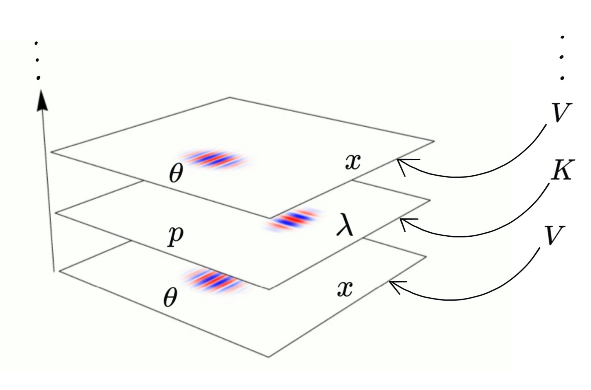
The employment of the appropriate basis at each step removes the need for arrows
| (77) | ||||
| (78) | ||||
| (79) | ||||
| (80) |
where the Fourier transform conform with Eq.(III) and Eq. (III) according to
| (81) | ||||
| (82) |
A schematic view of the sequence of steps (77)-(80) is shown in Fig. 4. Note that to maintain consistency, the propagator must be solely expressed in terms of contravariant components, e.g.,
| (83) |
The matrix exponentials in Eq. (77) can be evaluated analytically. For instance, assuming a two dimensional quantum system (ignoring and ) we obtain
| (84) |
with
| (85) | ||||
| (86) | ||||
| (87) | ||||
| (88) | ||||
| (89) | ||||
| (90) |
Having described the propagation for closed system Dirac evolution, we now proceed to introduce quantum dephasing (51), a particular open system interaction. According to Eq. (59), the dephasing dynamics enters into the exponential of the potential energy, thereby modifying the propagation step (79) as
| (98) |
with
| (99) |
The replacement of Eq. (79) by Eq. (98) is mathematically equivalent to Gaussian filtering along the momentum axis (i.e., convolution with a Gaussian in momentum) of the coherently propagated . This simple interpretation of the dephasing dynamics plays a crucial role in Sec. VI.
The presented algorithm can be implemented with the resources of a typical desktop computer and are well suited for GPU computing [110]. In particular, the illustration in the next section were executed with a Nvidia graphics card Tesla C2070.
VI Majorana Spinors
Hereafter, assuming a one dimensional dynamics, the Wigner function takes the functional form . Furthermore, natural units () are used throughout. In this section we employ a grid for and as well as a time step . Animations of simulations can be found in Ref. [111].
Majorana spinors, characterized for being their own antiparticles, are the subject of interest in a broad range of fields including high energy physics, quantum information theory and solid state physics [112]. In particular, the solid state counterpart of the relativistic Majorana spinors is known to be robust against perturbations and imperfections due to peculiar topological features [78].
In this section we study the dynamics of the original Majorana spinor [82] in the presence of dephasing noise (51). Let
| (100) |
be an arbitrary spinor, then there are two underlying Majorana states (see, e.g., Chapter 12, page 165 of Ref. [113])
| (101) |
In particular, we propagate the Majorana spinor [shown in Fig. 5(a)] obtained from
| (102) |
with and the numerical values , and the dephasing coefficient in natural units. The resulting time propagation of is shown in Fig. 5 (b).

Figure 5 reveals that the particle-antiparticle superposition of the Majorana state generates a strong interference in the phase space, which survives an even very intense dephasing interaction. The reason of such robustness is that both the particle component (with a positive momentum) and the antiparticle component (with a negative momentum) move in parallel along the positive spatial direction. This is in agreement with the interpretation of antiparticles as particles moving backwards in time. The interference fringes, consisting of negative and positive stripes, also remain parallel to the momentum axis. Considering the remark after Eq. (98), the action of dephasing is equivalent to the Gaussian filtering along the axis only. This mixes negative values with negative, positive values with positive, but never positive with negative values of the Wigner function. Hence, this leaves the interference stripes invariant. In other words, free Majorana spinors evolve in a decoherence-free subspace [114].
The described Majorana state dynamics is fundamentally different from the evolution of a cat-state, i.e., a particle-particle superposition. For example, up to a normalization factor, consider the following initial cat-state, composed of mostly particles:
| (103) |
Figure 6 depicts the evolution of this state under the influence of the same dephasing interaction as in Fig. 5. Contrary to the Majorana case, the negative momentum components of the cat state are made of particles; therefore, we observe in Fig. 6 that they move along the negative spatial direction. The interference stripes connecting the positive (moving to the right) and negative (moving to the left) momentum components no longer remain parallel with respect to the axis. Thus, dephasing occurs as the Gaussian filtering averages over positive and negative stripes, thereby washing interferences out.

We note that the distortion from the original Gaussian character of particle and atiparticle states at initial time in Figs. 5 and 6 is due to the momentum dispersion.
The total integrated negativity of the Wigner function
| (104) |
is widely regarded as a measurement of the quantum coherence because interferences are associated with Wigner function’s negative values.
Figure 7 shows that the negativity of the cat state reduces, while the negativity of the Majorana state is constant. Moreover, the negativity of the free Majorana spinor remains constant even for extreme values of the decoherences. Therefore, this robustness is not a perturbative effect with respect to the dephasing coefficient . Note that Majorana spinor’s initial negativity is more pronounced than that of the cat state (Fig. 7). Hence, Majorana states are more coherent than cat-states.
Having studied free evolution, we now proceed to a Majorana state evolving under the influence of the spatially modulated mass . This type of system also maintains a high coherence despite significant dephasing . The initial Majorana state is shown in Fig. 8 (a) while the propagated state at time is shown in Fig. 8 (b). The latter figure shows that interference is preserved. A comparison of the negativities for Majorana and cat-states as functions of time are shown in Fig. 9, where the Majorana state negativity oscillates albeit with some decay, which is much slower than the cat-state decay. Figure 10, showing the full Wigner dynamics, sheds light on the revival of the Majorana’s negativity: When the particle and antiparticle components merge and separate, the negativity disappears and appears, respectively. Furthermore, Majorana’s dynamics seems to be approximately constrained to a surface in the phase space and time, in contrast to the cat-state dynamics shown in Fig. 11.


VII Klein Tunneling
As the second numerical example, we examine the Klein paradox [115], an unexpected consequence of the Dirac equation, predicting that a positive energy particle colliding with a sharp potential barrier of the height is transmitted as a negative energy state. For example, the initial state (102) with , is shown in Fig. 12 (a) along with the potential .

We observe in Fig. 12 (b) that most of the wavepacket has been transmitted as antiparticles.
An important extension of the Klein paradox is the Klein tunneling, where the step potential is replaced by a finite width barrier. In this case, the theoretical prediction specifies a high transmission even for a wide barrier. Condensed matter analogies of this phenomenon are a subject of active research [7, 116]. Three snapshots of the Klein tunneling dynamics are shown in Fig. 13, where (a) corresponds to the positive energy initial state, (b) the state penetrating the potential barrier as antiparticle, and (c) the final state emerging from the barrier as particle.
The Dirac particle has a spinorial as well as a configurational degree of freedom. The Klein tunneling can be viewed as an interband transition between positive and negative energy states [117]. Analogous effects exist in non-relativistic dynamics. In particular, compared to the structureless case, non-relativitic systems with many degrees of freedom manifest many unique peculiarities such as, e.g., transmission rate enhancement [118, 119] and directional symmetry breaking [120]. Thus, the energy exchange between different degrees of freedom underlies the counterintuitive dynamics of both the Klein and the non-relativistic tunneling of particles with internal structure.
Furthermore, the Klein tunneling can be interpreted as the Landau-Zener transition between positive and negative energy states. This conclusion is obtained, e.g., by comparing Eqs. (B) and (138) (setting ) with Eqs. (19)-(21) in Ref. [121]. This observation underscores an analogy between solid state and relativistic physics.

Simulations with different values of the dephasing coefficient have been performed in order to investigate the effect of decoherence on the final transmission. Figure 14 depicts the integrated negativity (104) as a function of time for three different values of . The evolution without decoherence generates high negativity that indicates interference between the larger transmitted and smaller reflected wavepackets. In the same figure we observe that the decoherence eliminates negativity at later stages of the propagation.
Nevertheless, the effect of decoherence on the final transmission rate is small in Fig. 15, where the transmission as a function of time nearly coincides for different values of .
We also note a weak dependence of the antiparticle generation on the dephasing coefficient as shown in Fig. 16. Contrary to non-relativistic quantum dynamics [25, 28, 24, 40, 29, 30, 31, 90], decoherence in the relativistic regime does not recover a single particle classical description. Furthermore, we show in Appendix B that the limit of the Dirac equation leads to two classical Hamiltonians: One describing particles with a forward advancing clock (i.e., particles), while the other – a particle with backward flowing proper time (i.e., antiparticles). (This limit of the Dirac equation represents an example of classical Nambu dynamics [60].) This explains the persistence of positive energy states even for strong dephasing. We believe that the latter observation should also hold in condensed matter physics.
VIII Conclusions
We introduced the density matrix formalism for relativistic quantum mechanics as a generalization of the spinorial description of the Dirac equation. This formalism is employed to describe interactions with an environment. Moreover, we presented concise and effective numerical algorithms for the density matrix as well as the relativistic Wigner function propagation.
As a particularly important case, a Lindbland model of quantum dephasing was studied. While decoherence eliminated interferences, the particular structure of a free Majorana spinor remained robust. Partial robustness was also observed for a coordinate dependent mass term in the Dirac equation. This robustness represents yet another remarkable attribute of Majorana spinors [122] not presently acknowledged, which may be important experimentally. Moreover, the dynamics of the Klein paradox as well as Klein tunneling turned out to be weakly affected by quantum dephasing.
The presented numerical approach opens new horizons in a number of fields such as relativistic quantum chaos [123], the quantum-to-classical transition, and experimentally inspired relativistic atomic and molecular physics [124, 125, 126]. Additionally, our method can be used to simulate effective systems modeled by relativistic mechanics, e.g., graphene [127, 128], trapped ions [14], optical lattices [129], and semiconductors [130, 131]. Finally, the developed techniques can be generalized to treat Abelian [50, 132, 133] as well as non-Abelian [2, 134] (e.g., quark gluon) plasmas.
Acknowledgments. The authors thank Wojciech Zurek for insightful comments. R.C. is supported by DOE DE-FG02-02ER15344, D.I.B., and H.A.R. are partially supported by ARO-MURI W911NF-11-1-0268. A.C. acknowledges the support of the Fulbright Program. D.I.B. was also supported by 2016 AFOSR Young Investigator Research Program.
Appendix A Lorentz covariance of the Dirac equation
A vector in Feynman’s slash notation reads
| (105) |
where the gamma matrices obey the following Clifford algebra
| (106) |
with . The restricted Lorentz transform does not carry out reflections and preserves the direction of time and belongs to the group referred as . In the present case the transformation for the vector is carried out in terms of Lorentz spinors belonging to the double cover group of , according to
| (107) |
The concept of a spinor as an operator can be found for example in chapter 10 of Ref. [113]. The double cover of is known as the group and is precisely defined as
| (108) |
For this type of Lorentz transform the inverse can be obtained as [113]
| (109) |
The restricted Lorentz transform can also be carried out by the action of the complex special linear group [135, 136, 113], which is made of complex matrices with determinant one. The proper orthochronous Lorentz transformations can be parametrized by 6 variables denoting rotations and boots
| (110) |
where represent three rotation angles, three boosts (rapidity variables) and . The proper velocity can be obtained as the active boost of the proper velocity of a particle initially at rest with proper velocity . This means that in general it is possible to find a Lorentz spinor such that
| (111) |
This expression indicates that the information stored in the 4-vector can be carried out by the associated Lorentz rotor and the fixed reference 4-vector .
The Lorentz transformation in Eq. (107) implies that
| (112) |
Considering that transforms as the components of a covariant tensor, we obtain
| (113) |
which implies that
| (114) |
The Lorentz transformation of a vector field that depends on the spacetime position is carried out in a similar manner as (107)
| (115) |
Moreover, assuming that the origins of the reference frames coincide,
| (116) |
The Lorentz transformation of a spinorial field is consistent accordingly
| (117) |
The manifestly covariant Dirac equation is
| (118) |
such that applying the Lorentz rotor on the left we obtain
| (119) |
Employing Eq. (114), the first term of this equation can be written as
| (120) | ||||
| (121) |
Therefore, maintaining the form for the Dirac equation and demonstrating its relativistic covariance
| (122) |
Furthermore, it follows that the relativistic density matrix transforms as
| (123) | ||||
| (124) | ||||
| (125) | ||||
| (126) |
Appendix B The classical limit of the Dirac equation
The Dirac equation reads
| (127) |
In the classical limit, we understand the situation when the operators of the momenta and coordinates commute [137, 138, 44]. Following the Hilbert phase space formalism [44, 89], we separate the commutative and non-commutative parts of the Dirac generator by introducing the algebra of classical observables
| (128) | |||
| (129) |
which is connected with the quantum observables as
| (130) |
Substituting Eq. (130) into Eq. (127) and keeping the terms up to the zero-th order in , we get a function of and . Considering that and commute, we drop the hat hereafter such that
| (131) |
Utilizing the following unitary operator
| (132) |
| (133) |
we finally obtain
with
| (138) |
According to Eq. (138), the Dirac generator in the classical limit corresponds to a decoupled pair of classical time-extended Hamiltonians. The Hamiltonian describes the dynamics of a classical relativistic particle; while, governs the dynamics of a particle traveling backwards in time, which resembles an antiparticle. These conclusions confirm the results of numerical simulations in the main text, where a Dirac particle was coupled to a bath causing decoherence that physically realizes the limit.
References
- [1] W. Greiner, Relativistic quantum mechanics, vol. 3 (Springer, 1990).
- [2] H. Elze, M. Gyulassy, and D. Vasak, Phys. Lett. B 177, 402 (1986).
- [3] R. Hakim, Introduction to relativistic statistical mechanics (World Scientific, 2011).
- [4] A. Zee, Quantum field theory in a nutshell (Princeton university press, 2010).
- [5] A. Di Piazza, C. Müller, K. Z. Hatsagortsyan, and C. H. Keitel, Rev. Mod. Phys. 84, 1177 (2012).
- [6] K. Novoselov, A. K. Geim, S. Morozov, D. Jiang, M. Katsnelson, I. Grigorieva, S. Dubonos, and A. Firsov, Nature 438, 197 (2005).
- [7] M. Katsnelson, K. Novoselov, and A. Geim, Nat. Phys. 2, 620 (2006).
- [8] M. Z. Hasan and C. L. Kane, Rev. Mod. Phys. 82, 3045 (2010).
- [9] Q. Zhang and J. Gong, arXiv preprint arXiv:1510.06098 (2015).
- [10] J. Otterbach, R.G. Unanyan, and M. Fleischhauer, Phys. Rev. Lett. 102, 063602 (2009).
- [11] S. Ahrens, S.-Y. Zhu, J. Jiang, and Y. Sun, New J. Phys. 17, 113021 (2015).
- [12] J.Y. Vaishnav and C.W. Clark, Phys. Rev. Lett. 100, 153002 (2008).
- [13] O. Boada, A. Celi, J. Latorre, and M. Lewenstein, New J. Phys. 13, 035002 (2011).
- [14] R. Gerritsma, G. Kirchmair, F. Zähringer, E. Solano, R. Blatt, and C. Roos, Nature 463, 68 (2010).
- [15] R. Blatt and C. Roos, Nat. Phys. 8, 277 (2012).
- [16] J. Pedernales, R. Di Candia, D. Ballester, and E. Solano, New J. Phys. 15, 055008 (2013).
- [17] W. Liu, Phys. Chem. Chem. Phys. 14, 35 (2012).
- [18] J. Autschbach, J. Chem. Phys. 136, 150902 (2012).
- [19] R. Nandkishore, D. A. Huse, and S.L. Sondhi, Phys. Rev. B 89, 245110 (2014).
- [20] C. Gardiner and P. Zoller, Quantum noise, vol. 56 (Springer, 2004).
- [21] F. Petruccione and H.-P. Breuer, The theory of open quantum systems (Oxford Univ. Press, 2002).
- [22] M.S. Sarandy and D.A. Lidar, Phys. Rev. Lett. 95, 250503 (2005).
- [23] L. Viola, E. Knill, and S. Lloyd, Phys. Rev. Lett. 82, 2417 (1999).
- [24] W. H. Zurek, Rev. Mod. Phys. 75, 715 (2003).
- [25] W. H. Zurek, Phys. Today 44, 36 (1991).
- [26] S. L. Adler and A. Bassi, J. Phys. A 40, 15083 (2007).
- [27] Z. P. Karkuszewski, C. Jarzynski, and W. H. Zurek, Phys. Rev. Lett. 89, 170405 (2002).
- [28] W. H. Zurek, Phys. Scripta 1998, 186 (1998).
- [29] S. Habib, K. Jacobs, H. Mabuchi, R. Ryne, K. Shizume, and B. Sundaram, Phys. Rev. Lett. 88, 040402 (2002).
- [30] S. Habib, K. Jacobs, and K. Shizume, Phys. Rev. Lett. 96, 010403 (2006).
- [31] T. Bhattacharya, S. Habib, and K. Jacobs, Phys. Rev. A 67, 042103 (2003).
- [32] K. Jacobs and D. A. Steck, Contemp. Phys. 47, 279 (2006).
- [33] W. H. Zurek, Nat. Phys. 5, 181 (2009).
- [34] W. Zurek, Nature 412, 712 (2001).
- [35] I. V. Bazarov, Phys. Rev. ST Accel. Beams 15, 050703 (2012).
- [36] A. Gasbarro and I. Bazarov, Journal of synchrotron radiation 21, 289 (2014).
- [37] T. Tanaka, Phys. Rev. ST Accel. Beams 17, 060702 (2014).
- [38] D. Blokhintsev, The Philosophy of Quantum Mechanics (Springer, 2010).
- [39] E. J. Heller, J. Chem. Phys. 65, 1289 (1976).
- [40] S. Habib, K. Shizume, and W. H. Zurek, Phys. Rev. Lett. 80, 4361 (1998).
- [41] A. Bolivar, Quantum-classical correspondence (Springer Verlag, 2004).
- [42] C. Zachos, D. Fairlie, and T. Curtright, Quantum mechanics in phase space: an overview with selected papers (World Scientific, 2005).
- [43] R. Kapral, Ann. Rev. Phys. Chem. 57, 129 (2006).
- [44] D. I. Bondar, R. Cabrera, R. R. Lompay, M. Y. Ivanov, and H. A. Rabitz, Phys. Rev. Lett. 109, 190403 (2012).
- [45] A. Polkovnikov, Ann. Phys. 325, 1790 (2010).
- [46] E. Wigner, Phys. Rev. 40, 749 (1932).
- [47] T. Curtright, D. B. Fairlie, and C. K. Zachos, A Concise Treatise on Quantum Mechanics in Phase Space (World Scientific, 2013).
- [48] R. Hakim and J. Heyvaerts, Phys. Rev. A 18, 1250 (1978).
- [49] R. Hakim and H. Sivak, Ann. Phys. 139, 230 (1982).
- [50] D. Vasak, M. Gyulassy, and H. Elze, Ann. Phys. 173, 462 (1987).
- [51] Y. Yuan, K. Li, J. Wang, and K. Ma, Int. J. Theor. Phys. 49, 1993 (2010).
- [52] M. Kai, W. Jian-Hua, and Y. Yi, Chin. Phys. C 35, 11 (2011).
- [53] A. G. Campos, R. Cabrera, D. I. Bondar, and H. A. Rabitz, Phys. Rev. A 90, 034102 (2014).
- [54] R. Hudson, Rep. Math. Phys. 6, 249 (1974), ISSN 0034-4877.
- [55] V. V., N. Wiebe, F. C., and J. Emerson, New J. Phys. 15, 113037 (2013).
- [56] A. Mari and J. Eisert, Phys. Rev. Lett. 109, 230503 (2012).
- [57] I. Bialynicki-Birula, Acta Phys. Austriaca 151 (1977).
- [58] G.R. Shin and J. Rafelski, Phys. Rev. A 48, 1869 (1993).
- [59] A. Bolivar, J. Math. Phys. 42, 4020 (2001).
- [60] Y. Nambu, Physical Review D 7, 2405 (1973).
- [61] I. Bialynicki-Birula, P. Górnicki, and J. Rafelski, Phys. Rev. D 44, 1825 (1991).
- [62] G.R. Shin, I. Bialynicki-Birula, and J. Rafelski, Phys. Rev. A 46, 645 (1992).
- [63] I. Bialynicki-Birula, EPJ Web of Conferences 78, 01001 (2014).
- [64] F. Hebenstreit, A. Ilderton, M. Marklund, and J. Zamanian, Phys. Rev. D 83, 065007 (2011).
- [65] D. Berényi, S. Varró, P. Lévai, and V. V. Skokov, EPJ Web of Conferences 78, 03001 (2014).
- [66] A. Blinne and E. Strobel, Phys. Rev. D 93, 025014 (2016).
- [67] D. Kohen, C. Marston, and D. Tannor, J. Chem. Phys. 107, 5236 (1997).
- [68] D. I. Bondar, R. Cabrera, A. Campos, S. Mukamel, and H. A. Rabitz, J. Phys. Chem. Lett. 7, 1632 (2016), pMID: 27078510.
- [69] A. G. Campos, R. Cabrera, D. I. Bondar, and H. A. Rabitz, arXiv:1502.03025 (2016).
- [70] B. A. Bernevig and T. L. Hughes, Topological insulators and topological superconductors (Princeton University Press, 2013).
- [71] Z. Wang, A. Alexandradinata, R. J. Cava, and B. A. Bernevig, Nature 532, 189 (2016).
- [72] B. Lv, H. Weng, B. Fu, X. Wang, H. Miao, J. Ma, P. Richard, X. Huang, L. Zhao, G. Chen, et al., Phys. Rev. X 5, 031013 (2015).
- [73] H. Inoue, A. Gyenis, Z. Wang, J. Li, S. W. Oh, S. Jiang, N. Ni, B. A. Bernevig, and A. Yazdani, Science 351, 1184 (2016).
- [74] J. Alicea, Rep. Prog. Phys. 75, 076501 (2012).
- [75] A. Bühler, N. Lang, C. V. Kraus, G. Möller, S. D. Huber, and H. P. Büchler, Nat. Commun. 5 (2014).
- [76] S. Nadj-Perge, I. K. Drozdov, J. Li, H. Chen, S. Jeon, J. Seo, A. H. MacDonald, B. A. Bernevig, and A. Yazdani, Science 346, 602 (2014).
- [77] C. Nayak, S. H. Simon, A. Stern, M. Freedman, and S. Das Sarma, Rev. Mod. Phys. 80, 1083 (2008).
- [78] S. Albrecht, A. Higginbotham, M. Madsen, F. Kuemmeth, T. Jespersen, J. Nygård, P. Krogstrup, and C. Marcus, Nature 531, 206 (2016).
- [79] S. Diehl, E. Rico, M. A. Baranov, and P. Zoller, Nat. Phys. 7, 971 (2011).
- [80] J. C. Budich, S. Walter, and B. Trauzettel, Phys. Rev. B 85, 121405 (2012).
- [81] J. R. Wootton, J. Burri, S. Iblisdir, and D. Loss, Phys. Rev. X 4, 011051 (2014).
- [82] E. Majorana, Nuovo Cimento 14, 171 (1937).
- [83] T. A. Welton, Phys. Rev. 74, 1157 (1948).
- [84] W.E. Baylis and J. Huschilt”, Phys. Lett. A 301, 7 (2002).
- [85] A. Ilderton and G. Torgrimsson, Phys. Rev. D 88, 025021 (2013).
- [86] J. Eisert, M. Friesdorf, and C. Gogolin, Nat. Phys. 11, 124 (2015).
- [87] R. D. Sorkin, arXiv preprint gr-qc/9507057 (1995).
- [88] H.-P. Breuer and F. Petruccione, Relativistic Quantum Measurement and Decoherence: Lectures of a Workshop Held at the Istituto Italiano per gli Studi Filosofici Naples, April 9-10, 1999, vol. 559 (Springer Science & Business Media, 2000).
- [89] D. I. Bondar, R. Cabrera, D. V. Zhdanov, and H. A. Rabitz, Phys. Rev. A 88, 052108 (2013).
- [90] R. Cabrera, D. I. Bondar, K. Jacobs, and H. A. Rabitz, Phys. Rev. A 92, 042122 (2015).
- [91] M. Alcubierre, Introduction to 3+ 1 numerical relativity, vol. 2 (Oxford University Press Oxford, 2008).
- [92] F. Bopp, Ann. Inst. H. Poincaré 15 (1956).
- [93] M. Hillery, M. Scully, E. Wigner, et al., Phys, Rep. 106, 121 (1984).
- [94] M. A. Man’ko and V. I. Man’ko, Phys. Scripta 2012, 014020 (2012).
- [95] A. B. Migdal, Phys. Rev. 103, 1811 (1956).
- [96] D. Blokhintsev, J. Phys. U.S.S.R. 2, 71 (1940).
- [97] D. Blokhintsev and P. Nemirovsky, J. Phys. U.S.S.R. 3, 191 (1940).
- [98] D. Blokhintsev and Y. B. Dadyshevsky, Zh. Eksp. Teor. Fiz. 11, 222 (1941).
- [99] A. Caldeira and A. Leggett, Physica A 121, 587 (1983).
- [100] A. C. Doherty and K. Jacobs, Phys. Rev. A 60, 2700 (1999).
- [101] J. Dunkela and P. Hänggi, Phys. Rep. 471, 1 (2009).
- [102] B. Thaller, The Dirac equation, Texts and monographs in physics (Springer-Verlag, 1992).
- [103] G. R. Mocken and C. H. Keitel, Comp. Phys. Commun. 178, 868 (2008).
- [104] H. Bauke, M. Klaiber, E. Yakaboylu, K. Z. Hatsagortsyan, S. Ahrens, C. Müller, and C. H. Keitel, in SPIE Optics+ Optoelectronics (International Society for Optics and Photonics, 2013), pp. 87801Q–87801Q.
- [105] F. Fillion-Gourdeau, E. Lorin, and A. D. Bandrauk, Comput. Phys. Commun. 183, 1403 (2012).
- [106] R. Hammer and W. Pötz, Comp. Phys. Comm. 185, 40 (2014), ISSN 0010-4655.
- [107] R. Hammer, W. Pötz, and A. Arnold, J. Comp. Phys. 265, 50 (2014).
- [108] R. Beerwerth and H. Bauke, Comput. Phys. Commun. 188, 189 (2015).
- [109] M. Schreilechner and W. Pötz, arXiv preprint arXiv:1503.02685 (2015).
- [110] A. Klockner, N. Pinto, Y. Lee, B. Catanzaro, P. Ivanov, and A. Fasih, Parallel Computing 38, 157 (2012).
- [111]
Illustrative movies:
https://www.youtube.com/watch?v=gY0xpo-C02M
https://www.youtube.com/watch?v=uAsvmtfFhiU
https://www.youtube.com/watch?v=Dvso7GCUm6Y
https://www.youtube.com/watch?v=dX089esnAls . - [112] F. Wilczek, Nat. Phys. 5, 614 (2009).
- [113] P. Lounesto, Clifford algebras and spinors, vol. 286 (Cambridge university press, 2001).
- [114] D.A. Lidar, I. L. Chuang, and K. B. Whaley, Physical Review Letters 81, 2594 (1998).
- [115] W. Greiner, Relativistic quantum mechanics: wave equations (Springer Verlag, 2000).
- [116] A. F. Young and P. Kim, Nat. Phys. 5, 222 (2009).
- [117] P. E. Allain and J. Fuchs, Eur. Phys. J. 83, 301 (2011).
- [118] B. Zakhariev and S. Sokolov, Ann. Phys. 469, 229 (1964).
- [119] D. I. Bondar, W.-K. Liu, and M. Y. Ivanov, Phys. Rev. A 82, 052112 (2010).
- [120] I. Amirkhanov and B. N. Zakhariev, Sov. Phys. JETP 22 (1966).
- [121] E. Kane, J. Phys. Chem. Solids 12, 181 (1960).
- [122] S. R. Elliott and M. Franz, Rev. Mod. Phys. 87, 137 (2015).
- [123] R. Tomaschitz, J. Math. Phys. 32, 2571 (1991).
- [124] G. A. Mourou, T. Tajima, and S. V. Bulanov, Rev. Mod. Phys. 78, 309 (2006).
- [125] F. Krausz and M. Ivanov, Rev. Mod. Phys. 81, 163 (2009).
- [126] G. Sarri, W. Schumaker, A. Di Piazza, M. Vargas, B. Dromey, M. E. Dieckmann, V. Chvykov, A. Maksimchuk, V. Yanovsky, Z. H. He, et al., Phys. Rev. Lett. 110, 255002 (2013).
- [127] M. Müller, J. Schmalian, and L. Fritz, Phys. Rev. Lett. 103, 025301 (2009).
- [128] O. Morandi and F. Schürrer, J. Phys. A 44, 5301 (2011).
- [129] F. Dreisow, M. Heinrich, R. Keil, A. Tünnermann, S. Nolte, S. Longhi, and A. Szameit, Phys. Rev. Lett. 105, 143902 (2010).
- [130] J. Schliemann, D. Loss, and R. M. Westervelt, Phys. Rev. Lett. 94, 206801 (2005).
- [131] W. Zawadzki and T. M. Rusin, J. Phys. Condens. Matter 23, 143201 (2011).
- [132] J. Mendonça, Phys. Plasmas 18, 062101 (2011).
- [133] F. Haas, B. Eliasson, and P. K. Shukla, Phys. Rev. E 85, 056411 (2012).
- [134] H. Elze and U. Heinz, Phys. Rep. 183, 81 (1989).
- [135] W.E. Baylis, Phys. Rev. A 45, 4293 (1992).
- [136] W.E. Baylis, ed., ”Clifford (geometric) algebras with applications to physics, mathematics, and engineering” (Birkhauser, 1996).
- [137] P. Dirac, The principles of quantum mechanics (Clarendon, Oxford, 1958).
- [138] Y. M. Shirokov, Sov. J. Part. Nucl. 10, 1 (1979).