Calculation of dislocation positions and curved transition
pathways in BCC crystals from atomic displacements
Abstract
The thermodynamic description of dislocation glide in crystals depends crucially on the shape of the Peierls barrier that the dislocation has to overcome when moving in the lattice. While the height of this barrier can be obtained unequivocally using saddle-point search algorithms such as the Nudged Elastic Band (NEB) method, its exact shape depends on the chosen approximation of the transition pathway of the system. The purpose of this paper is to formulate a procedure that allows to identify the position of the dislocation directly from the displacements of atoms in its core. We investigate the performance of this model by calculating curved paths of a screw dislocation in tungsten from a series of images obtained recently using the NEB method at zero applied stress and for positive/negative shear stresses perpendicular to the slip direction. The Peierls barriers plotted along these curved paths are shown to be quite different from those obtained previously by assuming the straight dislocation path.
Keywords:
screw dislocation, BCC metal, dislocation pathway, Peierls barrier, Nudged Elastic Band.pacs
61.72.Hh, 02.60.-x, 45.10.DbI Introduction
Computational studies of dislocations in body-centered cubic (BCC) metals have been made using a wide variety of interatomic potentials and ab initio methods [1, 2, 3, 4, 5, 6, 7, 8, 9, 10, 11]. They view the evolution of the state of the system as its motion along an a priori unknown path in the configurational space spanned by the atomic degrees of freedom (DOF), where is the number of atoms in the simulated block. While this picture arises directly from molecular simulations, it presents severe difficulties when developing theoretical models of thermally activated glide of dislocations [12, 13], which serve to coarse-grain the atomistic results to the continuum. Not surprisingly, there has been a long-standing interest in developing approximate schemes to extract the effective position of the dislocation from the positions of atoms obtained by molecular statics simulations of single dislocations. While this approach is certainly attractive, it cannot be used without developing a systematic procedure that maps the atomic DOF to the position of the dislocation.
The most obvious choice that leads to the reduction of complexity of the system is to assume that the dislocation moves between two neighboring lattice sites along the straight line. This is implicitly assumed in most papers employing the Nudged Elastic Band (NEB) method [14, 15], where the position of the dislocation along the minimum energy path scales linearly with the image number [7, 11]. While the obtained barrier can be used to assess the stability of each intermediate state along the path, it does not constitute the Peierls barrier that could be used to develop thermodynamic models of dislocation glide such as that due to Dorn and Rajnak [12]. Moreover, a straight application of the NEB method to all DOF in the system leads to nonuniform distributions of dislocation positions among the images, which affects the shape of the obtained Peierls barrier [16]. A significant improvement of these results is obtained using our modification of the NEB method [16], where atomic relaxations are taken into account. This NEB+r method guarantees that the positions of the dislocation when following the minimum energy path are distributed uniformly among the images and thus the assumed proportionality between the dislocation position and the image number is justified. These developments have led to an accurate estimate of the Peierls barrier of screw dislocations in BCC W and its changes under the applied stress [16, 17]. However, these calculations are still based on the assumption that the path of the dislocation between two neighboring images is a straight line, which is not true in general.
In principle, it should be possible to deduce the dislocation position (and thus also its path between two positions in the lattice) directly from the displacements of atoms as obtained from molecular statics calculations or from the NEB (NEB+r) methods. This idea dates back to Peierls and Nabarro [18, 19], who associated the dislocation position with the point in the slip plane at which the displacement parallel to the slip direction, interpolated from the displacements of atoms, is equal to , where is the magnitude of the Burgers vector of the dislocation. Since then, this argument was used many times. In particular, it was adopted by Pizzagalli et al. [8], Rodney and Proville [10] and Proville et al. [20], where the position of the dislocation is defined by a single coordinate corresponding to the distance that the dislocation makes in a well-defined slip plane. The same level of approximation was also used by Ventelon et al. [21] in one of their methods (disregistry function method) that uses a combination of isotropic elasticity and geometry of the BCC lattice to define the position of the dislocation.
In general, the movement of the dislocation should be viewed as a three-dimensional event during which the center of the dislocation transits along a curved path in the vicinity of the slip plane. In attempt to resolve this path, Ventelon et al. [21] also proposed another model, whereby the dislocation position is identified using a cost function that is based on both the actual positions of atoms (as obtained from atomistic simulations) and the positions of atoms obtained from anisotropic elasticity for some trial dislocation position in the plane. The actual position of the dislocation is then obtained by minimizing this cost function that is defined as the distance between the two sets of coordinates in the five-dimensional subspace spanned by the coordinates of the five most displaced atoms around the dislocation. Since the position of the dislocation is determined by relative displacements of the three atoms closest to the dislocation in the direction parallel to the Burgers vector, a similar approach can be devised that is based on inversion of the Eshelby-Stroh sextic formalism (see, for example Hirth and Lothe [22]), which provides elastic displacements of atoms corresponding to a given position of the dislocation. We have investigated this possibility earlier (unpublished work). While this approximation can be used when the dislocation is in the middle of the lattice site formed by the nearest three atomic columns, it quickly worsens as the dislocation gets closer to any of these columns or the boundary between the neighboring lattice sites.
A different scheme whereby the position of the dislocation is determined by extrapolating differential displacements between the three atoms surrounding the dislocation into the interior of this triangle was developed by Itakura et al. [23]. This approach is closely related to a purely geometrical concept of barycentric (or trilinear) coordinates known from ternary diagrams that was originally applied to estimate the position of the dislocation by Heinrich and Schellenberger [24]. While this method makes use of the actual positions of atoms, the expression of the dislocation position as a linear combination of the displacements of the three nearest atoms in the direction parallel to the Burgers vector represents a convenient choice that is, however, not justified physically. This approximation was avoided in the recent work of Dezerald et al. [25] who aimed to reconstruct the two-dimensional Peierls barrier by interpolating the line energy of the dislocation, calculated by first principles, from two straight dislocation paths. One connects the neighboring potential minima in the plane and the other passes from an atom (“split-core” configuration) to the so-called “hard-core” position in the direction perpendicular to the first path. The Peierls potential is then expressed in the form of a Fourier series with the Fourier coefficients adjusted so as to minimize the least squares error between the calculated data and the Fourier series. The path of the dislocation between two neighboring minimum-energy lattice sites in the plane are obtained using the disregistry and cost function methods of Ventelon et al. [21]. While these paths are smooth, the corresponding Peierls barriers display sharp maxima for BCC Mo, W, Nb, while this is somewhat less pronounced for BCC Ta, V and ferromagnetic BCC Fe. This does not agree with the work of Suzuki et al. [26] and our more recent work (Ref. 27, 13), which show that in order to reproduce the experimentally measured temperature dependence of the flow stress, the Peierls potential has to possess a flat maximum.
In this paper, we develop a procedure that provides the position of a screw dislocation in BCC crystals (and thus the curved dislocation pathway) solely using the actual displacements of atoms in the dislocation core, without invoking isotropic or anisotropic elasticity. It generalizes the concept pioneered by Peierls and Nabarro [18, 19] in that it considers all three planes on which the dislocation can move. These calculations provide three lines whose intersection defines the position of the dislocation in the perpendicular plane. We demonstrate the performance of this method by calculating the paths of a straight screw dislocation in BCC W in the three possible planes from the discrete snapshots (images) of the system obtained recently using NEB+r calculations [17]. These calculations are made under zero applied stress and for positive and negative shear stresses perpendicular to the slip direction. We demonstrate that the shape of the Peierls barrier changes when considering the curved transition pathway of the dislocation as compared to that obtained previously by assuming the straight path of the dislocation between two equivalent minimum-energy configurations in the lattice [17].
II Complexity reduction
Let us consider that is the position of atom in the perfect lattice. Upon inserting a screw dislocation, applying additional displacements due to the externally applied load and relaxing the atoms, each atom moves into its new position, , where are atomic numbers. This configuration corresponds to the stable equilibrium (a minimum) with energy . In this configuration the dislocation is at the bottom of the Peierls valley for the applied stress . We will now consider that the dislocation has moved away from this minimum at constant applied stress , which is to say that all atoms were displaced from to . The energy of this new (nonequilibrium) configuration will be denoted . The enthalpy of the final state of the system relative to its initial state per unit length of the dislocation (or, simply, the line enthalpy of the dislocation) is then
| (1) |
where is the length of the dislocation segment contained in the simulated block.
The left-hand side of (1) seems to imply that the state of the system is described by the DOF associated with the positions of all particles. However, this is rather impractical from the computational point of view because, in this case, the energy of the system would have to be calculated from all atoms in the system.
To reduce this complexity, it is more convenient to separate the atomic degrees of freedom into two classes: (i) the minimum number of DOF that determine the position of the dislocation, and (ii) all remaining DOF that do not affect the position of the dislocation and thus they represent merely the large-scale response of the system to incorporating the dislocation. For this purpose, we can use the concept of the Burgers circuit to identify the region of the atomic block that contains the dislocation in its interior. When viewing a BCC crystal along the [111] direction, the shortest of these circuits passes through three atoms that are closest to the center of the dislocation. This implies that only 9 DOF are necessary to describe the dislocation position, while the remaining DOF represent the displacements of other atoms around the dislocation. However, the position of the dislocation is determined by relative displacements of the three atoms above in the direction of the Burgers vector. This reduces the 9 DOF to three, which are not all independent because their differences must sum up to the magnitude of the Burgers vector. Therefore, the information about the position of the dislocation is encoded in only two DOF.
The former suggests to find a procedure that maps the positions of atoms, , to the position of the intersection of the dislocation line with the perpendicular plane in the perfect lattice (called hereafter as the dislocation position), i.e.
| (2) |
It is important to emphasize that the former is defined in the deformed lattice with the dislocation, while the latter in the perfect lattice. If this mapping exists, the state of the system can be described using only two variables, the coordinates of the dislocation in the plane of the perfect lattice. 11 1 We implicitly assume that all other DOF are relaxed upon specifying the dislocation position. Hence, one can write the line enthalpy of the dislocation as
| (3) |
where the right-hand side is obtained from (1). Eq. (3) opens the possibility for developing a model of thermally activated dislocation glide, in which the transformation of the dislocation core is viewed as a motion of the center of the dislocation in the underlying Peierls potential.
For further developments, it will be convenient to introduce a transition pathway of the dislocation, , that is defined by a series of discrete points obtained from individual snapshots of the system as it moves along the minimum energy path. Hence, the left-hand side of (3) is equivalent to ,
| (4) |
where represents a particular point along a curved transition path of the dislocation. If the dislocation remains a straight line during this transition (which is the case at 0 K), we may express the line enthalpy of the dislocation as
| (5) |
where is the Peierls barrier 22 2 The minimum of the Peierls barrier for a given applied stress tensor is shifted to zero. and the second term is the work done by the applied stress on displacing the dislocation by the distance measured along the transition path. In the equation above, we have split the applied stress as , where contains only the shear stress acting in the slip plane parallel to the slip direction (i.e. the Schmid stress), whereas contains all other stresses. The latter are all stress components that do not exert a Peach-Koehler force on the dislocation. Clearly, the glide (Schmid) stress does work on displacing the dislocation, while non-glide stresses affect the shape of the Peierls barrier. The Peierls barrier can then be obtained from
| (6) |
Here, the first term on the right-hand side is obtained directly from the NEB (NEB+r) calculations, as it is evident by combining (1), (3) and (4). The expression (6) is completely general and can be used to obtain the shape of the Peierls barrier for an arbitrary applied load. For the sake of simplicity, we will consider in the following that . Hence, the NEB (NEB+r) calculations directly yield the line energies of the dislocation, , subject to a given non-glide stress .
III Position of the dislocation
Upon inserting the dislocation parallel to the axis, applying external load and relaxing the atomic positions, the atoms move from their perfect lattice positions, , into their new positions, . These two sets of atomic positions can be used to obtain a differential displacement map that uniquely identifies the lattice site with the dislocation. One such site corresponds to the gray triangle in Fig. 1 with the dislocation at some unknown position in this interior. The three planes on which the dislocation can move are marked in Fig. 1 as and distinguished by colors.

For each slip plane , we consider the two planes immediately above and below the lattice site with the dislocation, which are drawn in Fig. 1 by solid lines. 33 3 The planes above and below the lattice site with the dislocation refer to the two planes adjacent to this site. It is not important which of the two planes is considered as being “above” and which “below” this lattice site. Each of these planes is represented by a finite number of atoms , where , which are ordered such as to form chains. The displacement of each atom projected parallel to the Burgers vector of the dislocation is then defined as
| (7) |
where is the Burgers vector of the dislocation, and its magnitude. For the atoms far away from the dislocation core, the displacements approach constant values that represent the maximum and minimum of along the chain. Similarly as in Refs. 18, 19, the position of the dislocation in each chain , denoted hereafter , is assumed to coincide with the point along the chain, where the displacement in the direction parallel to the Burgers vector is half-way between its minima and maxima:
| (8) |
For each slip plane , this equation thus provides two estimates of the dislocation position, one for the chain of atoms above () and the other below () the lattice site with the dislocation. These points then define the line segments that are plotted in Fig. 1 by dashed lines. The actual position of the dislocation is associated with the intersection of these line segments. This is marked in Fig. 1 as the point . The implicit definition of using Eq. (8) is an approximation that, nevertheless, provides a good estimate of the position of the dislocation when it is at the body center of the shaded dislocation triangle in Fig. 1, i.e. when the system is in equilibrium at zero applied stress. This way of obtaining is adopted here for all states of the system along the minimum energy path irrespective of whether they represent equilibrium or nonequilibrium states.
(a)

(b)
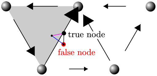
It should be pointed out that there is no a priori guarantee that the three line segments for will intersect at a single point. In general, one obtains three points that correspond to the intersections of three pairs of lines for the slip planes . This is illustrated in Fig. 2(a), where the shaded spheres correspond to the positions of atoms in the perfect lattice. The arrows are relative displacements of atoms between the image along the path for which the dislocation is closest to the boundary between the two lattice sites in Fig. 2(a) and the perfect lattice. The three edges of the small triangles are obtained from the method described above. In particular, the black edge in Fig. 2(a) lies along , purple along and blue along lines defined in Fig. 1. Each vertex of this small triangle, as well as any point in its interior, that are within the large gray triangle can be taken as representatives of the dislocation position. This is, however, not the case for the vertex marked “false node”, because it is outside of the gray lattice site determined by the differential displacement map. Fig. 2(b) shows the transition pathway predicted by the “true nodes” (black dots) and “false nodes” (red dots) from a series of images obtained by the NEB+r under zero applied stress [17]. The two sets of nodes coincide when the system is close to the beginning, end and the middle of the minimum energy path. For these images, the three line segments in Fig. 1 intersect at a single point and thus the dislocation positions are determined uniquely.
We define the transition pathway as a curve connecting the “true nodes” in Fig. 2(b). This is quite different from that obtained by the cost function method employed in Ref. 25 that is plotted by the green line (+ symbols). This deviation is the largest for the point in the middle of the path, which is determined uniquely by our method. Dezerald et al. [25] also show that the paths of the dislocation at zero applied stress obtained for various BCC metals are quite similar. This opens the possibility for a qualitative comparison of the dislocation pathway shown in Fig. 2(b) with Fig. 11 (data marked “DFT”) and Fig. 14 of Itakura et al. [23] for BCC Fe. The latter show that the energy of the dislocation is the lowest when positioned between the points marked (“hard-core” position) and in Fig. 2(b), which agrees well with the path predicted by our method.
The origin of the “false node” in Fig. 2(a) can be understood by looking at the displacements of the chain of atoms that are parallel to the boundary between these neighboring lattice sites (i.e. the blue lines in Fig. 1). These displacements are shown in Fig. 3 for two principally different atomic configurations. The first, marked “equilibrium state”, corresponds to the initial image along the path, where the dislocation is exactly at the body center of the gray triangle in Fig. 2(a). The second, marked “nonequilibrium state”, corresponds to the image in which the dislocation is closest to the boundary with the neighboring lattice site [case shown in Fig. 2(a)]. In the former, the displacements vary monotonously from their minimum at one end of the chain to their maximum at the other. In this case, the average displacement of atoms parallel to the Burgers vector is close to the inflection point of . Provided the system is close to equilibrium, the position of the dislocation along the chain can thus be safely determined using (8). For the nonequilibrium state, as the dislocation gets closer to the boundary between the two neighboring lattice sites, one atomic bond in the chain that coincides with this boundary becomes stretched to around . This is shown in Fig. 3 and this relative displacement of atoms is the bigger the closer the dislocation is to the boundary. In this case, the displacements of atoms do not vary monotonously along the chain. Instead, the sudden increase of displacements in the vicinity of the dislocation is followed by a gradual decay of the displacements, eventually reaching a constant value.

Because the position of the inflection point of cannot be determined with sufficient accuracy for nonequilibrium states, the linear approximation (8) may be a poor representation of the position . Due to the nonmonotonous character of it is also not advisable to look for higher order schemes. Instead, these observations suggest to make the prediction of the dislocation position only from two planes, excluding the one that is parallel to the boundary between the adjacent lattice sites (in Fig. 2, this is the case for corresponding to the blue edge of the small triangle). We have also checked that the jump in vs. does not appear if the dislocation position is obtained from the chain of atoms farther away from the lattice site with the dislocation. However, this leads to less accurate estimates of the dislocation position (larger triangle obtained by the intersection of with for ) and also to the drift of the dislocation position from the prediction made using the nearest chains of atoms in the three planes.
In all calculations made in this paper, the interactions between atoms were described using the Bond Order Potential (BOP) for BCC tungsten [28]. However, we have confirmed that the nonmonotonous character of the vs. curve in Fig. 3 is not specific to the potential used. This was found by calculating the dislocation pathway at zero applied stress with atomic interactions described by the Ackland-Thetford potential [29] for BCC Ta. This jump is also not caused by the mismatch betweeen the positions of the far-field atoms that are held fixed during the NEB (NEB+r) calculations and the actual position of the dislocation [8]. This was verified by doubling the radius of the cylindrical block used for the NEB simulation, which did not produce any noticeable change in the dependence of on . The jump is present in the data obtained from both NEB and NEB+r methods and in all atomic configurations, where the dislocation is close to the boundary between two adjacent lattice sites. It is also important to emphasize that the NEB methods do not impose any constraint to keep the Burgers vector of the dislocation constant during the search for the minimum energy path of the system. Owing to the above-mentioned misfit of atomic positions around the dislocation and in the far-field and rounding errors, it is theoretically possible that the relative displacements between the three atoms closest to the dislocation as obtained from the intermediate images obtained by NEB (NEB+r) calculations do not sum exactly to . We have checked this possibility for a few configurations, where the dislocation is very close to the edge of its lattice site. However, no significant deviation from the Burgers vector being exactly was detected.
Finally, an important insight is gained by calculating the dislocation positions when applying the stress directly in molecular statics calculations. In this case, pure shear stress parallel to the slip direction acting in the plane was applied in steps up to the value just before the dislocation moved (for details, see Ref. 9). For each relaxed atomic configuration at different applied stresses, we examined the dependence of vs. . Interestingly, all curves were smooth without any jump as observed from the NEB (NEB+r) calculations. Obviously, all atomic configurations obtained from direct molecular statics calculations are equilibrium states of the system at the given applied stress, while some intermediate images obtained using the NEB methods correspond to the unstable branch of the Peierls potential on which the dislocation moves spontaneously to its nearest minimum-energy configuration. As far as we can judge from our NEB+r calculations using 32 movable images, the origin of the jump in the vs. curve is associated with the inflection point of the Peierls barrier at which the dislocation can no longer be stabilized by the applied stress.
IV Numerical simulations
In our previous publication (Ref. 17), we used the NEB+r method [16] to investigate how the Peierls barrier of a screw dislocation in BCC W depends on the applied stress. In these calculations, the dislocation was assumed to move between two neighboring lattice sites along the straight line, which is a simplification that can now be removed. Our objective in the following is to use the calculated images that correspond to the minimum energy path of the system to: (i) identify the position of the dislocation in each image using the procedure formulated in the previous section, (ii) use these positions to determine the curved path of the dislocation on the three planes, and (iii) plot the energies of these snapshots along these curved paths to obtain the Peierls barriers.
We will first investigate how the shape of the dislocation pathway is affected by the shear stress perpendicular to the slip direction, . We carry out these calculations for three representative values of this stress, namely that is applied by imposing a uniform stress tensor in the coordinate system shown in Fig. 1 (for details, see Ref. 17). The calculated paths of the dislocation moving on the three planes in the zone and the three values of the shear stresses perpendicular to the slip direction are shown in Fig. 4. The large triangles represent the boundaries of four lattice sites – one from which the dislocation makes the jump (shaded) and the three others representing the target sites into which the dislocation moves by the glide on the three planes. The dislocation paths in bold are obtained as piecewise linear interpolations of the dislocation positions obtained for each image by the method developed above.

(a) (b) (c)

The Peierls barriers for the three planes and the three values of the shear stress perpendicular to the slip direction () are shown in the upper panels of Fig. 5. Here, dashed curves correspond to the barriers obtained in Ref. 17, where we considered that the dislocation moves between the two minima along the straight path. In this case, the transition coordinate is defined as , where are image numbers and the distance between neighboring minimum energy lattice sites in planes (Å). The solid curves are obtained by plotting , obtained from (6), along the paths identified using the procedure developed in Section III and shown in Fig. 4. Firstly, the three barriers for are identical, as dictated by symmetry, which is an important test of our procedure to calculate the dislocation pathway. The shape of the Peierls barrier changes significantly when drawn along the curved path. In particular, the panels for zero and positive show that the barriers in black that correspond to the glide of the dislocation on the plane are wider, with steeper gradient close to . The Peierls barrier thus deviates from the form to a parabolic or flat-top potentials that are often used to construct models of thermally activated dislocation glide [26, 13] (for a review, see the book of Caillard and Martin[30]). The right panel in Fig. 5 shows that the and barriers develop lower minima than the initial and final configurations along the path. These are probably consequences of the fact that the initial and final atomic positions are relaxed down to the maximum force on atom of only eV/Å.
For completeness, the lower panels of Fig. 5 show comparisons of the derivatives of these Peierls barriers. Here, we consider only those barriers that satisfy the fundamental equation , i.e. the dislocation moves on the plane (black curves, zero or positive ), or if it moves on the plane (purple curves, negative ). The curvature of the path shifts the peak of towards the beginning of the path. Qualitatively speaking, this shift together with the steep increase of the Peierls barrier close to will affect the activation enthalpy for the dislocation glide [12]. This can be demonstrated easily in the limit of zero applied stress for which the activated segment of the dislocation contains two isolated kinks between and (the length of the curved transition path of the dislocation). The energy of this activated state relative to that of the straight dislocation at the bottom of the Peierls valley is obtained from the Dorn-Rajnak model [Eq. (6) in Ref. 13 with and ] and reads
| (9) |
where eV/Å is the line tension of a straight dislocation[13]. We now use the two Peierls barriers shown in the middle panel of Fig. 5 together with (9) to obtain the predictions of the activation energy of a pair of noninteracting kinks at zero applied stress 44 4 Since , the energy in (9) can be closely approximated as .. These are eV if the dislocation is considered to move along a straight path and eV for the curved path of the dislocation [black path in Fig. 4(b)]. The latter is in excellent agreement with the value eV obtained in Ref. 13 from the experimental data, where the thermal component of the flow stress vanishes. The curvature of the dislocation pathway and the associated flat maximum of the Peierls barrier will also give rise to larger curvature of the stress dependence of the activation enthalpy [12, 13] and thus to a steep increase of the flow stress with decreasing temperature, as observed universally in all BCC metals.
V Conclusions
We have developed a numerical scheme that provides the position of the center of the dislocation only from the knowledge of the displacements of atoms between the relaxed configuration and the perfect lattice. This represents a generalization of the model devised originally by Peierls and Nabarro [18, 19]. Our model goes beyond these developments in that it provides two components of the dislocation position, one of which lies in the glide plane, whereas the other is perpendicular to this plane.
The position of the dislocation in each of the three possible slip planes is identified as the point, where the displacement of atoms parallel to the slip direction is half-way between its minima and maxima. This calculation is made separately for the chain of atoms above and below the lattice site with the dislocation. For each slip plane, one thus obtains two points that define a line with possible positions of the dislocation. The pairwise intersections of the three lines thus obtained define the corners of a triangle that approximates the position of the dislocation. We have shown that one edge of this triangle is ill-defined when the dislocation is very close to the boundary between the adjacent lattice site. However, the dislocation path obtained from the intersections of the two remaining edges is smooth and the dislocation positions agree with differential displacement maps as well as with DFT calculations made by Itakura et al. [23].
We have demonstrated this procedure by calculating the path of the dislocation between two minimum energy lattice sites, using the snapshots of atomic positions obtained from our recent NEB+r calculations made in Ref. 17. These calculations have been made for all three planes on which the dislocation can move and for zero, positive and negative shear stresses perpendicular to the slip direction. The curvature of the dislocation path is shown to affect the shape of the Peierls barrier, which becomes steeper close to the beginning and end of the transition path and, at the same time, more flat close to its maximum. This shape will affect macroscopic predictions, such as the temperature dependence of the yield stress. In particular, we expect that the activation enthalpy will be a stronger function of the applied stress, which will give rise to a steeper increase of the flow stresses with decreasing temperature.
Acknowledgements.
The author thanks Vaclav Vitek for fruitful discussions on the topic. This research was supported by the Marie-Curie International Reintegration Grant No. 247705 “MesoPhysDef” and by the Academy of Sciences of the Czech Republic, Project no. RVO:68081723. This work has been carried out at the Central European Institute of Technology (CEITEC) with research infrastructure supported by the project CZ.1.05/1.1.00/02.0068 financed from the EU Structural Funds.References
- [1] V. Vitek, R. C. Perrin, and D. K. Bowen, Philos. Mag. 21, 1049 (1970).
- [2] W. Xu and J. A. Moriarty, Comp. Mater. Sci. 9, 348 (1998).
- [3] C. Woodward and S. I. Rao, Philos. Mag. A 81, 1305 (2001).
- [4] S. L. Frederiksen and K. W. Jacobsen, Philos. Mag. 83, 365 (2003).
- [5] J. Li, C.-Z. Wang, J.-P. Chang, W. Cai, V. V. Bulatov, K.-M. Ho, and S. Yip, Phys. Rev. B 70, 1 (2004).
- [6] M. Cawkwell, D. Nguyen-Manh, C. Woodward, D. G. Pettifor, and V. Vitek, Science 309, 1059 (2005).
- [7] L. Ventelon and F. Willaime, J. Comp.-Aid. Mat. Design 14, 85 (2007).
- [8] L. Pizzagalli, P. Beauchamp, and H. Jónsson, Philos. Mag. 88, 91 (2008).
- [9] R. Gröger, A. G. Bailey, and V. Vitek, Acta Mater. 56, 5401 (2008).
- [10] D. Rodney and L. Proville, Phys. Rev. B 79, 094108 (2009).
- [11] M. Mrovec, D. Nguyen-Manh, C. Elsässer, and P. Gumbsch, Phys. Rev. Lett. 106, 246402 (2011).
- [12] J. E. Dorn and S. Rajnak, Trans. AIME 230, 1052 (1964).
- [13] R. Gröger and V. Vitek, Acta Mater. 56, 5426 (2008).
- [14] H. Jónsson, G. Mills, and K. W. Jacobsen, Classical and Quantum Dynamics in Condensed Phase Simulations (World Scientific, 1998), chap. 16. Nudged elastic band method for finding minimum energy paths of transitions, pp. 385–404.
- [15] G. Henkelman and H. Jónsson, J. Chem. Phys. 113, 9978 (2000).
- [16] R. Gröger and V. Vitek, Model. Simul. Mater. Sci. Eng. 20, 035019 (2012).
- [17] R. Gröger and V. Vitek, Acta Mater. 61, 6362 (2013).
- [18] R. Peierls, Proc. Phys. Soc. 52, 34 (1940).
- [19] F. R. N. Nabarro, Proc. Phys. Soc. 59, 256 (1947).
- [20] L. Proville, L. Ventelon, and D. Rodney, Phys. Rev. B 87, 144106 (2013).
- [21] L. Ventelon, F. Willaime, E. Clouet, and D. Rodney, Acta Mater. 61, 3973 (2013).
- [22] J. P. Hirth and J. Lothe, Theory of dislocations (J.Wiley & Sons, New York, 1982), 2nd ed.
- [23] M. Itakura, M. Kaburaki, and M. Yamaguchi, Acta Mater. 60, 3698 (2012).
- [24] R. Heinrich and W. Schellenberger, Phys. Stat. Sol. B 47, 81 (1971).
- [25] L. Dezerald, L. Ventelon, E. Clouet, C. Denoual, D. Rodney, and F. Willaime, Phys. Rev. B 89, 024104 (2014).
- [26] T. Suzuki, H. Koizumi, and H. O. K. Kirchner, Acta Metall. Mater. 43, 2177 (1995).
- [27] R. Gröger, Ph.D. thesis, University of Pennsylvania (2007), URL http://arxiv.org/abs/0707.3577.
- [28] M. Mrovec, R. Gröger, A. G. Bailey, D. Nguyen-Manh, C. Elsässer, and V. Vitek, Phys. Rev. B 75, 104119 (2007).
- [29] G. J. Ackland and R. Thetford, Philos. Mag. A 56, 15 (1987).
- [30] D. Caillard and J. L. Martin, Thermally activated mechanisms in crystal plasticity (Pergamon Press, 2003).