跳到论文正文
W Papers独立论文阅读器 arXiv:1409.0830 论文正文 计算阅读时间 · 0%
引用这篇论文根据当前论文元数据生成,正式投稿前建议核对。


License: arXiv.org perpetual non-exclusive license
arXiv:1409.0830v2 [math.GT] 19 Oct 2015

The distribution of gaps for saddle connections on the octagonThanks: August 24, 2026Thanks: Both authors acknowledge support from U.S. National Science Foundation grants DMS 1107452, 1107263, 1107367 “RNMS: GEometric structures And Representation varieties” (the GEAR Network). The first author was partially supported by the NSF grants of Ilya Kapovich (DMS-1405146) and Christopher J. Leininger (DMS-1207183). The second author was partially supported by the NSF grant of Jayadev Athreya (DMS-1351853).

Caglar Uyanik and Grace Work Address: Department of Mathematics, University of Illinois at Urbana-Champaign, 1409 West Green Street, Urbana, IL 61801, USA
https://sites.google.com/site/caglaruyanik/
http://www.math.uiuc.edu/˜work2
Email address: cuyanik2@illinois.edu Email address: work2@illinois.edu
Abstract.

We explicitly compute the limiting gap distribution for slopes of saddle connections on the flat surface associated to the regular octagon with opposite sides identified. This is the first such computation where the Veech group of the translation surface has multiple cusps. We also show how to parametrize a Poincaré section for the horocycle flow on S​L​(2,ℝ)/S​L​(X,ω)SL(2,\mathbb{R})/SL(X,\omega) associated to an arbitrary Veech surface (X,ω)(X,\omega). As a corollary, we show that the associated gap distribution is piecewise real analytic.

1. Introduction

1.1. Gap distribution for the Octagon

Consider the surface 𝒪\mathcal{O} obtained by identifying parallel sides of the regular octagon by Euclidean translations, as shown in Figure 1. This results in a genus 2 translation surface with a single cone point of cone angle 6​π6\pi. A saddle connection on this surface is a straight line connecting the cone point to itself. To each saddle connection, γ\gamma, we associate a holonomy vector, vγ∈ℂv_{\gamma}\in\mathbb{C}, that records how far it travels in each direction. For example, the saddle connection drawn in Figure 1 would have holonomy vector 2​(1+2)+i2(1+\sqrt{2})+i.

11γ\gamma
Figure 1. The regular octagon with parallel sides identified to obtain the translation surface 𝒪\mathcal{O}. A saddle connection γ\gamma has been drawn connecting the cone point to itself.

We are interested in the slopes of holonomy vectors coming from the saddle connections on the octagon. Following the convention introduced by [1, 2], we refer to them as “slopes of saddle connections”. Since the set of vectors is symmetric with respect to coordinate axes, we restrict our attention to slopes in the first quadrant.

Let

𝕊𝒪={slope(vγ)=Im⁡(vγ)Re⁡(vγ)∣γ is a saddle connection on 𝒪 and 0<Re(vγ),0≤Im(vγ)}\mathbb{S}_{\mathcal{O}}=\left\{\slope(v_{\gamma})=\frac{\im(v_{\gamma})}{\re(v_{\gamma})}\mid\text{$\gamma$ is a saddle connection on $\mathcal{O}$ and}\ 0<\re(v_{\gamma}),0\leq\im(v_{\gamma})\right\}

We write 𝕊𝒪\mathbb{S}_{\mathcal{O}} as an increasing union of 𝕊𝒪R\mathbb{S}_{\mathcal{O}}^{R} for R→∞R\to\infty, where

𝕊𝒪R:={slope(vγ)∣γ is a saddle connection on 𝒪 and 0<Re(vγ)≤R,0≤Im(vγ)≤R}.\mathbb{S}^{R}_{\mathcal{O}}:=\left\{\slope(v_{\gamma})\mid\text{$\gamma$ is a saddle connection on $\mathcal{O}$ and}\ 0<\re(v_{\gamma})\leq R,0\leq\im(v_{\gamma})\leq R\right\}.

In other words, 𝕊𝒪R\mathbb{S}_{\mathcal{O}}^{R} is the set of (finite) non-negative slopes of saddle connections on 𝒪\mathcal{O} that lie in the first quadrant and in the ℓ∞\ell_{\infty} ball of radius RR around the origin. Let N⁡(R)=|𝕊𝒪R|N(R)=|\mathbb{S}^{R}_{\mathcal{O}}| be the cardinality of the set 𝕊𝒪R\mathbb{S}^{R}_{\mathcal{O}}. Veech showed that N⁡(R)N(R) grows quadratically with RR, moreover the saddle connection directions on any Veech surface (X,ω)(X,\omega), in particular 𝒪\mathcal{O}, equidistribute on S1S^{1} with respect to Lebesgue measure on the circle, see [12].

Write 𝕊𝒪R\mathbb{S}_{\mathcal{O}}^{R} as a set of increasing slopes:

𝕊𝒪R={0≤s0R<s1R<s2R<⋯<sN⁡(R)−1R}.\mathbb{S}_{\mathcal{O}}^{R}=\left\{0\leq s_{0}^{R}<s_{1}^{R}<s_{2}^{R}<\cdots<s_{N(R)-1}^{R}\right\}.

Since N⁡(R)N(R) grows quadratically, it is natural to define the set of renormalized slope gaps for 𝒪\mathcal{O} as

𝔾𝒪R:={R2(siR−si−1R):1≤i≤N(R)−1,si∈𝕊𝒪R}.\mathbb{G}_{\mathcal{O}}^{R}:=\left\{R^{2}(s_{i}^{R}-s_{i-1}^{R}):1\leq i\leq N(R)-1,s_{i}\in\mathbb{S}_{\mathcal{O}}^{R}\right\}.

Our main theorem describes the asymptotic behavior for the distribution of the set of renormalized slope gaps:

Theorem 1.1.

There is a limiting probability distribution function f:[0,∞)→[0,1]f:[0,\infty)\to[0,1] such that

limR→∞|𝔾𝒪R∩(a,b)|N⁡(R)=∫abf⁡(x)​𝑑x.\lim_{R\to\infty}\frac{|\mathbb{G}_{\mathcal{O}}^{R}\cap(a,b)|}{N(R)}=\int_{a}^{b}f(x)dx.

The function ff is continuous, piecewise differentiable with seven points of non-differentiability. Each piece is expressed in terms of elementary functions. The graph of the function ff is shown below and an explicit description is given in Section 3.2.

Figure 2. Limiting gap distribution for the octagon

Theorem 1.1 gives information on finer statistics for the set of slopes of saddle connections. In particular, it reveals an underlying structure because we see that the gap distribution is not exponential and has quadratic tail. Were the slopes of saddle connections “truly random”, one would expect the gap distribution to be exponential, as is the case with independent identically distributed uniform random variables on [0,1][0,1].

1.2. Translation Surfaces

In this section we review the necessary background related to translation surfaces, which we use in Theorem 1.2. We refer reader to [6, 7, 8, 14] for a detailed treatment of the subject. A translation surface is a pair (X,ω)(X,\omega) where XX is a closed Riemann surface of genus gg, and ω\omega is a holomorphic 11-form on XX. Equivalently, a translation surface is a finite union of polygons {P1,…​Pk}\{P_{1},\dotsc P_{k}\} in the Euclidean plane such that for each edge there exists a parallel edge of the same length and these pairs are glued together by a Euclidean translation. It follows that the total angle around each vertex is equal to 2​π​ci2\pi c_{i} for some integer ci≥1c_{i}\geq 1. We note here that we are considering a fixed embedding of the above polygons into ℝ2≅ℂ\mathbb{R}^{2}\cong\mathbb{C} up to translations, that is we are considering polygons in the Euclidean plane with a preferred vertical direction. Since translations are holomorphic functions that preserve the standard one form d​zdz on the Euclidean plane, we get a Riemann surface structure on the glued surface together with a holomorphic 11-form. The set of vertices where the total angle θ>2​π\theta>2\pi is called the set of cone points, and each cone point corresponds to a zero of the holomorphic 11-form. At a zero of order nn the total angle is 2​π​(n+1)2\pi(n+1).

A saddle connection is a geodesic connecting two of the cone points without any cone points in the interior. An oriented saddle connection γ\gamma in XX determines a holonomy vector

vγ=∫γωv_{\gamma}=\int_{\gamma}\omega

which records the direction and the length of the saddle connection γ\gamma. We will denote the set of holonomy vectors corresponding to saddle connections in (X,ω)(X,\omega) by Λs​c​(X,ω)\Lambda_{sc}(X,\omega). Given a translation surface (X,ω)(X,\omega) the set Λs​c​(X,ω)\Lambda_{sc}(X,\omega) is a discrete subset of ℝ2\mathbb{R}^{2}, with the property that g​Λs​c​(X,ω)=Λs​c​g​(X,ω)g\Lambda_{sc}(X,\omega)=\Lambda_{sc}g(X,\omega), see [6, 7, 13].

A translation surface XX comes with a set of topological data, the genus, the set of zeros, and the multiplicities of zeros. By the Gauss-Bonnet theorem the sum of the order of the zeros is equal to 2​g−22g-2 where gg is the genus of the surface XX. Therefore, the topological data can be represented by a vector α→=(α1,…,αm)\vec{\alpha}=(\alpha_{1},\dotsc,\alpha_{m}) where αi\alpha_{i} is the order of the it​hi^{th} zero. We say that two translation surfaces are equivalent if there is an orientation preserving isometry between them which preserves the preferred vertical direction. Given a topological data α→\vec{\alpha} the moduli space ℋ⁡(α→)\mathcal{H}(\vec{\alpha}) of translation surfaces up to above equivalence relation is called a stratum.

There is a natural S​L​(2,ℝ)SL(2,\mathbb{R}) action on the space of translation surfaces: Given a translation surface (X,ω)(X,\omega), which is a finite union of polygons {P1,…,Pk}\{P_{1},\dotsc,P_{k}\}, and a matrix A∈S​L​(2,ℝ)A\in SL(2,\mathbb{R}), A⋅(X,ω)A\cdot(X,\omega) is the translation surface defined by the union of polygons {A​P1,…,A​Pk}\{AP_{1},\dotsc,AP_{k}\}. It is easy to see that the S​L​(2,ℝ)SL(2,\mathbb{R}) action preserves the topological data, so it induces an action on each strata ℋ⁡(α→)\mathcal{H}(\vec{\alpha}).

The stabilizer of (X,ω)(X,\omega) under the S​L​(2,ℝ)SL(2,\mathbb{R}) action on the space of translation surfaces is denoted by S​L​(X,ω)SL(X,\omega). Equivelantly, S​L​(X,ω)SL(X,\omega) is the the group of derivatives of the orientation preserving affine diffeomorphisms (X,ω)(X,\omega). We will call the stabilizer S​L​(X,ω)SL(X,\omega) the Veech group of (X,ω)(X,\omega). We note here that some authors call the image of S​L​(X,ω)SL(X,\omega) in ℙ​S​L​(2,ℝ)\mathbb{P}SL(2,\mathbb{R}), denoted by ℙ​S​L​(X,ω)\mathbb{P}SL(X,\omega), the Veech group, but we will stick to the notation of Smillie-Ulcigrai in [10]. A translation surface (X,ω)(X,\omega) is called a Veech surface if S​L​(X,ω)SL(X,\omega) has finite covolume, i.e. S​L​(2,ℝ)/S​L​(X,ω)SL(2,\mathbb{R})/SL(X,\omega) has finite volume.

The image of the Veech group Γ𝒪\Gamma_{\mathcal{O}} of the octagon in ℙ​S​L​(2,ℝ)\mathbb{P}SL(2,\mathbb{R}) is isomorphic to the triangle group Δ⁡(4,∞,∞)\Delta(4,\infty,\infty). The presence of multiple cusps gives rise to new computational challenges but also gives a conjectural idea of how to handle the general case where the Veech group has arbitrarily many cusps. Hence the computation of the gap distribution on 𝒪\mathcal{O} gives yet another step towards formulating and proving a general statement about gap distributions of saddle connections on any Veech surface. Indeed, in Theorem 1.2 we give an effective way of parametrizing a Poincaré section to the horocycle flow on S​L​(2,ℝ)/S​L​(X,ω)SL(2,\mathbb{R})/SL(X,\omega) where the Veech group S​L​(X,ω)SL(X,\omega) has arbitrarily many cusps.

1.3. Poincaré section for a general Veech surface

Let (X,ω)(X,\omega) be a Veech surface, such that S​L​(X,ω)SL(X,\omega) has n<∞n<\infty cusps. We further assume here that the Veech group contains −I​d-Id; in Section 4 we remove this assumption and prove a theorem for the general case. It is well known that the set of saddle connections Λs​c​(X,ω)\Lambda_{sc}(X,\omega) on (X,ω)(X,\omega) can be decomposed into finitely many S​L​(X,ω)SL(X,\omega) orbits of saddle connections, see [6]. Let Λs​cs​h​o​r​t(X,ω):=⊔i=1nSL(X,ω)⋅wi⊂Λs​c(X,ω)\Lambda_{sc}^{short}(X,\omega):=\sqcup_{i=1}^{n}SL(X,\omega)\cdot w_{i}\subset\Lambda_{sc}(X,\omega) be a set of shortest saddle connections in any given direction, so that any saddle connection on (X,ω)(X,\omega) is parallel to exactly one element of Λs​cs​h​o​r​t​(X,ω)\Lambda_{sc}^{short}(X,\omega). Let us denote Λs​cwi​(X,ω)=S​L​(X,ω)⋅wi\Lambda_{sc}^{w_{i}}(X,\omega)=SL(X,\omega)\cdot w_{i}. Consider the set

ΩM={g​S​L​(X,ω)∣g⁡(X,ω)​ has a horizontal saddle connection of length ≤1}.\Omega^{M}=\{gSL(X,\omega)\mid g(X,\omega)\text{ has a horizontal saddle connection of length $\leq 1$}\}.

According to [1], ΩM\Omega^{M} is a Poincaré section for the action of horocycle flow on the moduli space S​L​(2,ℝ)/S​L​(X,ω)SL(2,\mathbb{R})/SL(X,\omega). By definition of ⊔i=1nΛs​cwi(X,ω)\sqcup_{i=1}^{n}\Lambda_{sc}^{w_{i}}(X,\omega) we can write

ΩM=Ω1M∪⋯∪ΩnM,\Omega^{M}=\Omega_{1}^{M}\cup\cdots\cup\Omega_{n}^{M},

where

ΩiM={g​S​L​(X,ω)∣g​Λs​cwi​(X)∩(0,1]≠∅},\Omega_{i}^{M}=\{gSL(X,\omega)\mid g\Lambda_{sc}^{w_{i}}(X)\cap(0,1]\neq\emptyset\},

is the set of elements g​S​L​(X,ω)gSL(X,\omega) in the S​L​(2,ℝ)SL(2,\mathbb{R}) orbit of the Veech group, such that g​Λs​cwi​(X)g\Lambda_{sc}^{w_{i}}(X) contains a horizontal saddle connection of length ≤1\leq 1.

Let Γ1,…,Γn\Gamma_{1},\dotsc,\Gamma_{n} be maximal parabolic sugroups of S​L​(X,ω)SL(X,\omega) representing the conjugacy classes of all maximal parabolic subgroups in S​L​(X,ω)SL(X,\omega). Each Γi\Gamma_{i} is isomorphic to ℤ⊕ℤ/2​ℤ\mathbb{Z}\oplus\mathbb{Z}/2\mathbb{Z}. Pick a generator PiP_{i} for the infinite cyclic factor of Γi\Gamma_{i} with eigenvalue 11. It follows from [11] that, each wiw_{i} in the above decomposition can be chosen so that wiw_{i} is an eigenvector for PiP_{i}.

Conjugate the parabolic elements Pi∈ΓiP_{i}\in\Gamma_{i} with an element CiC_{i} in S​L​(2,ℝ)SL(2,\mathbb{R}) such that

Si=Ci​Pi​Ci−1=[1αi01].S_{i}=C_{i}P_{i}C_{i}^{-1}=\left[\begin{array}[]{cc}1&\alpha_{i}\\ 0&1\end{array}\right].

Moreover, CiC_{i} can be chosen so that Ci⋅wi=[10]C_{i}\cdot w_{i}=\left[\begin{array}[]{c}1\\ 0\end{array}\right]. Define Ma,bM_{a,b} and sets Ωi\Omega_{i} as follows

Ma,b=[ab0a−1],M_{a,b}=\left[\begin{array}[]{cc}a&b\\ 0&a^{-1}\end{array}\right],

where a≠0,ba\neq 0,b are real numbers, and

Ωi:={(a,b)∈ℝ2∣0<a≤1​and​ 1−(αi)​a<b≤1}.\Omega_{i}:=\{(a,b)\in\mathbb{R}^{2}\mid 0<a\leq 1\ \text{and}\ 1-(\alpha_{i})a<b\leq 1\}.
Theorem 1.2.

Let (X,ω)(X,\omega) be a Veech surface such that the Veech group S​L​(X,ω)SL(X,\omega) has n<∞n<\infty cusps. There are coordinates from the section ΩM\Omega^{M} to the set ⨆i=1nΩi\bigsqcup_{i=1}^{n}\Omega_{i}. More precisely, the bijection between S​L​(2,ℝ)/S​L​(X,ω)SL(2,\mathbb{R})/SL(X,\omega) and S​L​(2,ℝ)⋅(X,ω)SL(2,\mathbb{R})\cdot(X,\omega) sends ΩiM\Omega_{i}^{M} to {Ma,b​Ci​(X,ω)∣(a,b)∈Ωi}\{M_{a,b}C_{i}(X,\omega)\mid(a,b)\in\Omega_{i}\}, and the latter set is bijectively parametrized by Ωi\Omega_{i}. The return time function is piecewise rational with pieces defined by linear equations in these coordinates. The limiting gap distribution for any Veech surface is piecewise real analytic.

Acknowledgements.

The authors are grateful to their respective advisors Chris Leininger and Ilya Kapovich, and Jayadev Athreya for their constant support, advice and encouragement. We would like to thank Samuel Lelièvre for his willingness to answer our questions and very useful discussions. We would like to thank J.D. Quigley for his aid in creating and debugging our sage code. We would also like to thank Zeev Rudnick for helpful comments on an earlier version of this paper. In addition, we thank the anonymous referee for his/her suggestions.

2. Veech Groups and Gaps

2.1. The Octagon and the normalized LL

Recall that the image of the Veech group Γ𝒪\Gamma_{\mathcal{O}} of the octagon in ℙ​S​L​(2,ℝ)\mathbb{P}SL(2,\mathbb{R}) is isomorphic to the triangle group Δ⁡(4,∞,∞)\Delta(4,\infty,\infty). The group Γ𝒪\Gamma_{\mathcal{O}}, as calculated by Smillie-Ulcigrai in [10], is generated by the following two matrices:

ρ=[12−121212]σ=[12​(1+2)01]\rho=\left[\begin{array}[]{c c}\frac{1}{\sqrt{2}}&\frac{-1}{\sqrt{2}}\\ \frac{1}{\sqrt{2}}&\frac{1}{\sqrt{2}}\end{array}\right]\hskip 72.26999pt\sigma=\left[\begin{array}[]{c c}1&2(1+\sqrt{2})\\ 0&1\end{array}\right]

The matrix

T=[1002]​[1(1+2)01]=[1(1+2)02]∈G​L​(2,ℝ)T=\left[\begin{array}[]{c c}1&0\\ 0&\sqrt{2}\end{array}\right]\left[\begin{array}[]{c c}1&(1+\sqrt{2})\\ 0&1\end{array}\right]=\left[\begin{array}[]{c c}1&(1+\sqrt{2})\\ 0&\sqrt{2}\end{array}\right]\in GL(2,\mathbb{R})

transforms 𝒪\mathcal{O} into ℒ\mathcal{L}, see Figure 3.

112\sqrt{2}1+21+\sqrt{2}11
Figure 3. The Veech surface ℒ\mathcal{L}

We carry out the computations for the Veech surface ℒ\mathcal{L}.

Note that if the limiting gap distribution of a translation surface XX is given by

limR→01N⁡(R)​|𝔾XR∩(a,b)|=∫abf⁡(x)​𝑑x\lim_{R\rightarrow 0}\frac{1}{N(R)}|\mathbb{G}_{X}^{R}\cap(a,b)|=\int_{a}^{b}f(x)dx

then the limiting gap distribution for c​XcX, with c∈ℝc\in\mathbb{R} will be given by

limR→∞1N⁡(c​R)​|𝔾c​Xc​R∩(a,b)|=1c4​∫abf⁡(xc2)​𝑑x.\lim_{R\rightarrow\infty}\frac{1}{N(cR)}|\mathbb{G}_{cX}^{cR}\cap(a,b)|=\frac{1}{c^{4}}\int_{a}^{b}f\left(\frac{x}{c^{2}}\right)dx.

In order to see this, we observe that scaling does not change the slopes, hence we have

𝕊XR=𝕊c​Xc​R={0≤s0R<s1R<⋯<sN⁡(R)−1R}\mathbb{S}_{X}^{R}=\mathbb{S}_{cX}^{cR}=\left\{0\leq s_{0}^{R}<s_{1}^{R}<\cdots<s_{N(R)-1}^{R}\right\}

where we now have to consider slopes in a ball of radius c​RcR about the origin. Thus the set of slope gaps is renormalized by (c​R)2(cR)^{2} so,

𝔾c​Xc​R={(cR)2(siR−si−1R:1≤N(R)−1,si∈𝕊XR}.\mathbb{G}_{cX}^{cR}=\left\{(cR)^{2}(s_{i}^{R}-s_{i-1}^{R}:1\leq N(R)-1,s_{i}\in\mathbb{S}_{X}^{R}\right\}.

Therefore we are interested in computing

limR→∞1N⁡(c​R)​|𝔾c​Xc​R∩(a,b)|\displaystyle\lim_{R\rightarrow\infty}\frac{1}{N(cR)}\left|\mathbb{G}_{cX}^{cR}\cap(a,b)\right| =limR→∞1N⁡(c​R)⋅N⁡(R)N⁡(R)​|{c2​R2​(siR−si−1R)}∩(a,b)|\displaystyle=\lim_{R\rightarrow\infty}\frac{1}{N(cR)}\cdot\frac{N(R)}{N(R)}\left|\{c^{2}R^{2}(s_{i}^{R}-s_{i-1}^{R})\}\cap(a,b)\right|
=limR→∞1N⁡(c​R)⋅N⁡(R)N⁡(R)​|{R2​(siR−si−1R)}∩(a/c2,b/c2)|\displaystyle=\lim_{R\rightarrow\infty}\frac{1}{N(cR)}\cdot\frac{N(R)}{N(R)}\left|\{R^{2}(s_{i}^{R}-s_{i-1}^{R})\}\cap(a/c^{2},b/c^{2})\right|
=1c2​∫a/c2b/c2f⁡(x)​𝑑x\displaystyle=\frac{1}{c^{2}}\int_{a/c^{2}}^{b/c^{2}}f(x)dx

Applying a change of variables then yields the desired result.

We can write the matrix TT, which transforms 𝒪\mathcal{O} to ℒ\mathcal{L}, as c​gcg, where g∈S​L​(2,ℝ)g\in SL(2,\mathbb{R}), since

21/4​[121/400221/4]=[1002].2^{1/4}\left[\begin{array}[]{cc}\frac{1}{2^{1/4}}&0\\ 0&\frac{\sqrt{2}}{2^{1/4}}\end{array}\right]=\left[\begin{array}[]{cc}1&0\\ 0&\sqrt{2}\end{array}\right].

As we show in Section 3.1, the distribution of gaps is preserved under the S​L​(2,ℝ)SL(2,\mathbb{R}) action, hence the limiting gap distribution for 𝒪\mathcal{O} and ℒ\mathcal{L} is related by the aforementioned formula with c=121/4c=\frac{1}{2^{1/4}}.

Conjugating the Veech group Γ𝒪\Gamma_{\mathcal{O}} of the octagon by the transformation TT, gives the following generators for the Veech group Γ\Gamma of ℒ\mathcal{L}:

R=[1+2−(2+2) 1−1]S=[12+201]R=\left[\begin{array}[]{c c}1+\sqrt{2}&-(2+\sqrt{2})\\ \ 1&-1\end{array}\right]\hskip 72.26999ptS=\left[\begin{array}[]{c c}1&2+\sqrt{2}\\ 0&1\end{array}\right]

where RR is a finite order elliptic element and SS is an infinite order parabolic element. By building a fundamental domain, we also see that SS generates the stabilizier of the infinity in ℙ​S​L​(ℒ)\mathbb{P}SL(\mathcal{L}).

2.2. Gap Distributions

Let 𝕊ℒR:={0=s0R<s1R<s2R<⋯<sN⁡(R)−1R}\mathbb{S}_{\mathcal{L}}^{R}:=\left\{0=s_{0}^{R}<s_{1}^{R}<s_{2}^{R}<\cdots<s_{N(R)-1}^{R}\right\} be the set of slopes of saddle connections on the translation surface ℒ\mathcal{L} that lie in the first quadrant and in the ball of radius RR around the origin with respect to ℓ∞\ell_{\infty} metric. Let

𝔾ℒR:={R2(siR−si−1R):1≤i≤N(R)−1,si∈𝕊ℒR}\mathbb{G}_{\mathcal{L}}^{R}:=\left\{R^{2}(s_{i}^{R}-s_{i-1}^{R}):1\leq i\leq N(R)-1,s_{i}\in\mathbb{S}_{\mathcal{L}}^{R}\right\}

be the set of renormalized slope gaps. Recall that the main goal of this paper to compute the following limit:

limR→∞|𝔾ℒR∩(a,b)|N⁡(R).\lim_{R\rightarrow\infty}\frac{|\mathbb{G}_{\mathcal{L}}^{R}\cap(a,b)|}{N(R)}.

To evaluate this limit we translate the gap distribution question into one about the return time of the horocycle flow to a Poincaré section. For the purpose of this paper, horocycle flow will be defined by the action of the subgroup

{hs=[10−s1]:s∈ℝ}.\left\{h_{s}=\left[\begin{array}[]{cc}1&0\\ -s&1\end{array}\right]:s\in\mathbb{R}\right\}.

This definition was chosen so that it acts on slopes by translations. That is, if we consider a vector vv with slope σ\sigma, then the slope of hs⋅vh_{s}\cdot v will be σ−s\sigma-s. The key step in the strategy is the construction of an appropriate Poincaré section for the horocycle flow. That is, a set Ω\Omega such that under the horocycle flow the orbit of almost every point in moduli space intersects Ω\Omega in a countable discrete set of times. The cross section we choose is the set of translation surfaces in the S​L​(2,ℝ)SL(2,\mathbb{R}) orbit of the ℒ\mathcal{L} with a short horizontal saddle connection. If we apply horocycle flow to one of these surfaces, we see that the next saddle connection to become horizontal, is the saddle connection with short horizontal component and smallest slope, and the return time to the Poincaré section is exactly its slope.

3. Moduli Space, Poincaré Section, Computations

We now prove Theorem 1.1 generalizing a strategy used by Athreya, Cheung in [3] and Athreya, Chaika, Lelièvre in [2].

3.1. Poincaré Section

It is well-known [6] that for a Veech surface (X,ω)(X,\omega) the set Λs​c​(X,w)\Lambda_{sc}(X,w) of saddle connections can be written as a union of finitely many disjoint S​L​(X,ω)SL(X,\omega) orbits of saddle connections. In other words, there are finitely many vectors v1,…,vn∈ℝ2v_{1},\dotsc,v_{n}\in\mathbb{R}^{2} such that

Λs​c​(X,ω)=⋃i=1nS​L​(X,ω)​vi.\Lambda_{sc}(X,\omega)=\bigcup_{i=1}^{n}SL(X,\omega)v_{i}.

In our case, where the Veech surface (X,ω)(X,\omega) is ℒ\mathcal{L}, we have 4 disjoint orbits:

Λs​c​(ℒ)=Γ​[10]∪Γ​[2+10]∪Γ​[01]∪Γ​[02]\Lambda_{sc}(\mathcal{L})=\Gamma\left[\begin{array}[]{cc}1\\ 0\end{array}\right]\cup\Gamma\left[\begin{array}[]{cc}\sqrt{2}+1\\ 0\end{array}\right]\cup\Gamma\left[\begin{array}[]{cc}0\\ 1\end{array}\right]\cup\Gamma\left[\begin{array}[]{cc}0\\ \sqrt{2}\end{array}\right]

where the first two orbits and the last two orbits are pairwise parallel. Therefore, it suffices to consider only shorter orbits:

Λs​ch​(ℒ):=Γ​[10],Λs​cv​(ℒ):=Γ​[01].\Lambda_{sc}^{h}(\mathcal{L}):=\Gamma\left[\begin{array}[]{cc}1\\ 0\end{array}\right],\ \Lambda_{sc}^{v}(\mathcal{L}):=\Gamma\left[\begin{array}[]{cc}0\\ 1\end{array}\right].

It follows from the work of Athreya [1], that the set ΩM={g​Γ∣g​Λs​c​(ℒ)∩(0,1]≠∅}\Omega^{M}=\{g\Gamma\mid g\Lambda_{sc}(\mathcal{L})\cap(0,1]\neq\emptyset\} is a Poincaré section for the action of the horocycle flow hsh_{s} on the space M=S​L​(2,ℝ)/ΓM=SL(2,\mathbb{R})\big/\Gamma. The observation above allows us to write ΩM=ΩhM∪ΩvM\Omega^{M}=\Omega_{h}^{M}\cup\Omega_{v}^{M} where

ΩhM={g​Γ∣g​Λs​ch​(ℒ)∩(0,1]≠∅}\displaystyle\Omega_{h}^{M}=\{g\Gamma\mid g\Lambda_{sc}^{h}(\mathcal{L})\cap(0,1]\neq\emptyset\}
ΩvM={g​Γ∣g​Λs​cv​(ℒ)∩(0,1]≠∅}.\displaystyle\Omega_{v}^{M}=\{g\Gamma\mid g\Lambda_{sc}^{v}(\mathcal{L})\cap(0,1]\neq\emptyset\}.

For a Veech surface (X,ω)(X,\omega) the S​L​(2,ℝ)SL(2,\mathbb{R}) orbit of (X,ω)(X,\omega) can be identified with the moduli space S​L​(2,ℝ)/S​L​(X,ω)SL(2,\mathbb{R})/SL(X,\omega). In what follows, and in Section 4, we will implicitly use this identification. Hence, in this setting, ΩM=ΩhM∪ΩvM\Omega^{M}=\Omega_{h}^{M}\cup\Omega_{v}^{M} is the set of translation surfaces in the S​L​(2,ℝ)SL(2,\mathbb{R}) orbit of ℒ\mathcal{L} with a horizontal saddle connection of length ≤1\leq 1.

Now, we will give a parametrization of the section ΩM\Omega^{M} in ℝ2\mathbb{R}^{2}. We first need the following matrix: Let

Ma,b=[ab0a−1],M_{a,b}=\left[\begin{array}[]{cc}a&b\\ 0&a^{-1}\end{array}\right],

where a≠0,ba\neq 0,b are real numbers.

Next define the following subsets of ℝ2\mathbb{R}^{2}:

Ω1={(a,b)∈ℝ2∣0<a≤1​and​ 1−(2+2)​a<b≤1}\displaystyle\Omega_{1}=\{(a,b)\in\mathbb{R}^{2}\mid 0<a\leq 1\ \text{and}\ 1-(\sqrt{2}+2)a<b\leq 1\}
Ω2={(a,b)∈ℝ2∣0<a≤1​and​ 1−a<b≤1}\displaystyle\Omega_{2}=\{(a,b)\in\mathbb{R}^{2}\mid 0<a\leq 1\ \text{and}\ 1-a<b\leq 1\}

Let ℒR=Rπ/2​ℒ=[01−10]​ℒ\mathcal{L}^{R}=R_{\pi/2}\mathcal{L}=\left[\begin{smallmatrix}0&1\\ {-1}&0\end{smallmatrix}\right]\mathcal{L} be the translation surface obtained from ℒ\mathcal{L} by a rotation by π/2\pi/2 in the clockwise direction. The Veech group ΓR\Gamma_{R} of ℒR\mathcal{L}^{R} can be obtained by conjugating the Veech group of ℒ\mathcal{L}. Hence ΓR\Gamma_{R} is generated by

Rπ/2​(R)​Rπ/2−1=[1+2−1 2+2−1]Rπ/2​(−R​S−1)​Rπ/2−1=[1101].R_{\pi/2}(R)R^{-1}_{\pi/2}=\left[\begin{array}[]{c c}1+\sqrt{2}&-1\\ \ 2+\sqrt{2}&-1\end{array}\right]\hskip 72.26999ptR_{\pi/2}(-RS^{-1})R^{-1}_{\pi/2}=\left[\begin{array}[]{c c}1&1\\ 0&1\end{array}\right].
Theorem 3.1.

There are coordinates from the section ΩhM∪ΩvM\Omega_{h}^{M}\cup\Omega_{v}^{M} to the set Ω1∪Ω2\Omega_{1}\cup\Omega_{2}. More precisely, the canonical bijection Θ:S​L​(2,ℝ)/Γ→S​L​(2,ℝ)⋅ℒ\Theta:SL(2,\mathbb{R})/\Gamma\to SL(2,\mathbb{R})\cdot\mathcal{L} sends ΩhM\Omega_{h}^{M} to {Ma,b​ℒ∣(a,b)∈Ω1}\{M_{a,b}\mathcal{L}\mid(a,b)\in\Omega_{1}\} and ΩvM\Omega_{v}^{M} to {Ma,b​ℒR∣(a,b)∈Ω2}\{M_{a,b}\mathcal{L}^{R}\mid(a,b)\in\Omega_{2}\}, and the latter sets are bijectively parametrized by Ω1\Omega_{1} and Ω2\Omega_{2}. In these coordinates, the return time function R:Ω1∪Ω2→ℝ>0R:\Omega_{1}\cup\Omega_{2}\to\mathbb{R}_{>0}, defined by

R⁡(a,b)={min⁡{s∣hs​Ma,b​ℒ∈ΩhM∪ΩvM}for (a,b)∈Ω1min⁡{s∣hs​Ma,b​ℒR∈ΩhM∪ΩvM}for (a,b)∈Ω2R(a,b)=\left\{\begin{array}[]{ll}\min\{s\mid h_{s}M_{a,b}\mathcal{L}\in\Omega_{h}^{M}\cup\Omega_{v}^{M}\}&\text{for $(a,b)\in\Omega_{1}$}\\ \min\{s\mid h_{s}M_{a,b}\mathcal{L}^{R}\in\Omega_{h}^{M}\cup\Omega_{v}^{M}\}&\text{for $(a,b)\in\Omega_{2}$}\end{array}\right.

is a piecewise rational function with five pieces, which is uniformly bounded below by 11. The return map T:Ω1∪Ω2→Ω1∪Ω2T:\Omega_{1}\cup\Omega_{2}\to\Omega_{1}\cup\Omega_{2} is a measure preserving bijection and it is piecewise linear with countably many pieces.

Refer to caption
Refer to caption
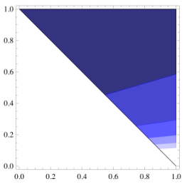
Figure 4. Source regions for the return map. Colors represent finer subdivisions corresponding to different values of the constant in each equation. White areas indicate infinitely many subdivisions following the same pattern as the others in the region.
Refer to caption
Refer to caption
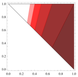
Figure 5. Target regions for the return map. Each colored region from the source maps to the same colored region in the target.
Proof.

Suppose that g​Γ∈ΩhMg\Gamma\in\Omega_{h}^{M}. We need to show that g​ℒ=Ma,b​ℒg\mathcal{L}=M_{a,b}\mathcal{L} for some (a,b)∈Ω1(a,b)\in\Omega_{1}. By definition g​ℒg\mathcal{L} has a horizontal saddle connection [a0]\left[\begin{array}[]{cc}a\\ 0\end{array}\right] such that

[a0]=g​γ​[10]\left[\begin{array}[]{cc}a\\ 0\end{array}\right]=g\gamma\left[\begin{array}[]{cc}1\\ 0\end{array}\right]

for some γ∈Γ,\gamma\in\Gamma, and 0<a≤10<a\leq 1. Since Γ\Gamma acts on Λs​ch​(ℒ)\Lambda_{sc}^{h}(\mathcal{L}) transitively and for any element γ∈Γ\gamma\in\Gamma we have g​γ​ℒg\gamma\mathcal{L}=g​ℒg\mathcal{L}, we can assume that

[a0]=g⁡[10].\left[\begin{array}[]{cc}a\\ 0\end{array}\right]=g\left[\begin{array}[]{cc}1\\ 0\end{array}\right].

The elements in S​L​(2,ℝ)SL(2,\mathbb{R}) which take [10]\left[\begin{array}[]{cc}1\\ 0\end{array}\right] to [a0]\left[\begin{array}[]{cc}a\\ 0\end{array}\right] are precisely of the form

Ma,b=[ab0a−1].M_{a,b}=\left[\begin{array}[]{c c}a&b\\ 0&a^{-1}\end{array}\right].

Thus, every element in ΩhM\Omega_{h}^{M} can be written as Ma,b​ℒM_{a,b}\mathcal{L} for some (a,b)(a,b) where 0<a≤10<a\leq 1. Since the element S=[12+201]S=\left[\begin{array}[]{c c}1&2+\sqrt{2}\\ 0&1\end{array}\right] is in the Veech group Γ\Gamma, and

Ma,b​S−n=[ab−(2+2)​a​n0a−1],M_{a,b}S^{-n}=\left[\begin{array}[]{c c}a&b-(2+\sqrt{2})an\\ 0&a^{-1}\end{array}\right],

we can write every element g​ℒg\mathcal{L} in ΩhM\Omega_{h}^{M} as Ma,b​ℒM_{a,b}\mathcal{L} where (a,b)∈Ω1(a,b)\in\Omega_{1}.

For any point (a,b)∈Ω1(a,b)\in\Omega_{1}, it is clear that Ma,b​ℒM_{a,b}\mathcal{L} has a short horizontal, the image of the saddle connection [10]\left[\begin{array}[]{cc}1\\ 0\end{array}\right].

Finally, we prove that Ω1\Omega_{1} bijectively parametrizes {Ma,b​ℒ∣(a,b)∈Ω1}\{M_{a,b}\mathcal{L}\mid(a,b)\in\Omega_{1}\}. We suppose that (a,b),(c,d)∈Ω1(a,b),(c,d)\in\Omega_{1} and that Ma,b​ℒ=Mc,d​ℒM_{a,b}\mathcal{L}=M_{c,d}\mathcal{L}, and must prove that (a,b)=(c,d)(a,b)=(c,d). We have

Ma,b​Mc,d−1=[acb​c−a​d0ca]∈Γ,M_{a,b}M_{c,d}^{-1}=\left[\begin{array}[]{cc}\frac{a}{c}&bc-ad\\ 0&\frac{c}{a}\end{array}\right]\in\Gamma,

which fixes infinity in the upper half-plane. As we noted in Section 2.1, the stabilizer of infinity in P​S​L​(ℒ)PSL(\mathcal{L}) is the infinite cylic group generated by the matrix

S=[12+201].S=\left[\begin{array}[]{c c}1&2+\sqrt{2}\\ 0&1\end{array}\right].

Since a/c>0a/c>0 it follows that a=ca=c. From this we see that 1−(2+2)​a<b,d≤11-(2+\sqrt{2})a<b,d\leq 1, and (b−d)​a=k⁡(2+2)(b-d)a=k(2+\sqrt{2}), which implies b=db=d, and hence (a,b)=(c,d)(a,b)=(c,d), as required.

Now suppose that g​Γ∈ΩvMg\Gamma\in\Omega_{v}^{M}. We need to show that g​ℒ=Ma,b​ℒRg\mathcal{L}=M_{a,b}\mathcal{L}^{R} for some (a,b)∈Ω2(a,b)\in\Omega_{2}. By definition, there is a horizontal saddle connection [a0]\left[\begin{array}[]{cc}a\\ 0\end{array}\right] on g​ℒg\mathcal{L} such that

[a0]=g​γ​[01].\left[\begin{array}[]{cc}a\\ 0\end{array}\right]=g\gamma\left[\begin{array}[]{cc}0\\ 1\end{array}\right].

As in the previous case, we can assume that

[a0]=g⁡[01].\left[\begin{array}[]{cc}a\\ 0\end{array}\right]=g\left[\begin{array}[]{cc}0\\ 1\end{array}\right].

This implies that

Rπ/2−1​g​[01]=[0a].R_{\pi/2}^{-1}g\left[\begin{array}[]{cc}0\\ 1\end{array}\right]=\left[\begin{array}[]{cc}0\\ a\end{array}\right].

The elements in S​L​(2,ℝ)SL(2,\mathbb{R}) that take [01]\left[\begin{array}[]{cc}0\\ 1\end{array}\right] to [0a]\left[\begin{array}[]{cc}0\\ a\end{array}\right] are precisely of the form [a−10ba]\left[\begin{array}[]{c c}a^{-1}&0\\ b&a\end{array}\right]. This means that

g​ℒ=Rπ/2​[a−10ba]​ℒ=Rπ/2​[a−10ba]​Rπ/2−1​Rπ/2​ℒ=[a−b0a−1]​ℒR,g\mathcal{L}=R_{\pi/2}\left[\begin{array}[]{c c}a^{-1}&0\\ b&a\end{array}\right]\mathcal{L}=R_{\pi/2}\left[\begin{array}[]{c c}a^{-1}&0\\ b&a\end{array}\right]R_{\pi/2}^{-1}R_{\pi/2}\mathcal{L}=\left[\begin{array}[]{c c}a&-b\\ 0&a^{-1}\end{array}\right]\mathcal{L}^{R},

which implies that every element g​ℒ∈Ω2Mg\mathcal{L}\in\Omega_{2}^{M} can be written as Ma,b​ℒRM_{a,b}\mathcal{L}^{R} for 0<a≤10<a\leq 1. Observe that the matrix

Rπ/2​(−R​S−1)​Rπ/2−1=[1101]∈ΓR=Rπ/2​Γ​Rπ/2−1,R_{\pi/2}(-RS^{-1})R^{-1}_{\pi/2}=\left[\begin{array}[]{c c}1&1\\ 0&1\end{array}\right]\in\Gamma_{R}=R_{\pi/2}\Gamma R^{-1}_{\pi/2},

the Veech group of ℒR\mathcal{L}^{R}. Thus, arguing as in the first case, we can write every element g​ℒ∈Ω2Mg\mathcal{L}\in\Omega_{2}^{M} as Ma,b​ℒRM_{a,b}\mathcal{L}^{R} for (a,b)∈Ω2(a,b)\in\Omega_{2}. The bijection between Ω2\Omega_{2} and {Ma′,b′​ℒR∣(a′,b′)∈Ω2}\{M_{a^{\prime},b^{\prime}}\mathcal{L}^{R}\mid(a^{\prime},b^{\prime})\in\Omega_{2}\} now follows from a similar argument as in the case of Ω1\Omega_{1}.

We now compute the return time function R:Ω1∪Ω2→ℝ>0R:\Omega_{1}\cup\Omega_{2}\to\mathbb{R}_{>0} explicitly. Recall that for a given point Ma,b​ℒM_{a,b}\mathcal{L} the return time to the section under the horocycle flow is given by the smallest positive slope of the saddle connection on Ma,b​ℒM_{a,b}\mathcal{L} with horizontal component ≤1\leq 1. Therefore we must determine the associated slope for each point (a,b)∈Ω(a,b)\in\Omega. This requires finding the original saddle connection whose image has the smallest positive slope.

On the original ℒ\mathcal{L} there are 4 different saddle connections of interest, shown in Figure 6. We determined the set of points (a,b)(a,b) such that under the matrix Ma,bM_{a,b} each of the four saddle connections of interest has horizontal component less than 11 and greater than 00, in other words, that it is a candidate to have the smallest slope. This divides Ω1\Omega_{1} into four subregions, these are shown in Figure 7.

GGCCBBDDHHFFEEAA
Figure 6. The saddle connections of interest
Refer to caption
Figure 7. Subregions

On the overlap of the red and green regions, the saddle connections coming from A​HAH and B​DBD are possible candidates. To check which one dominates, we consider their slopes. The slope of Ma,b⋅A​HM_{a,b}\cdot AH is 1a​b\frac{1}{ab} and the slope of Ma,b⋅B​DM_{a,b}\cdot BD is 1a⁡(a+b)\frac{1}{a(a+b)}. If a,b>0a,b>0, we have a+b>ba+b>b so a⁡(a+b)>a​ba(a+b)>ab and therefore 1a⁡(a+b)<1a​b\frac{1}{a(a+b)}<\frac{1}{ab} which implies that the image of B​DBD dominates the image of A​HAH, so A​HAH must end where B​DBD appears, at the line b=1−ab=1-a.

On the overlap of the green and yellow regions, we see the saddle connections coming from B​DBD and H​FHF. Again comparing slopes, we have the slope of Ma,b⋅H​FM_{a,b}\cdot HF is 2a⁡(a⁡(2+1)+b​2)\frac{\sqrt{2}}{a(a(\sqrt{2}+1)+b\sqrt{2})}. Since

a>0,a+b+a2>a+b​ and so ​1a⁡(a+b+a2)<1a⁡(a+b),a>0,a+b+\frac{a}{\sqrt{2}}>a+b\text{ and so }\frac{1}{a\left(a+b+\frac{a}{\sqrt{2}}\right)}<\frac{1}{a(a+b)},

therefore H​FHF dominates B​DBD.

On the overlap of the green and purple regions, we see the saddle connections coming from B​DBD and A​EAE. The slope of Ma,b⋅A​EM_{a,b}\cdot AE is 1a⁡((1+2)​a+b)\frac{1}{a((1+\sqrt{2})a+b)}. Since a>0a>0, we have

a+2​a+b>a+b​ so ​1a⁡((1+2)​a+b)<1a⁡(a+b),a+\sqrt{2}a+b>a+b\text{ so }\frac{1}{a((1+\sqrt{2})a+b)}<\frac{1}{a(a+b)},

thus A​EAE dominates B​DBD.

On the overlap of purple and yellow we see the saddle connections coming from A​EAE and H​FHF. Since a>0a>0, we have

a+2​a+b>a+b+a2​ so ​1a+2​a+b<1a+b+a2a+\sqrt{2}a+b>a+b+\frac{a}{\sqrt{2}}\text{ so }\frac{1}{a+\sqrt{2}a+b}<\frac{1}{a+b+\frac{a}{\sqrt{2}}}

and thus A​EAE dominates H​FHF.

One can show, using similar arguments and direct computation, that these four saddle connections are the only ones whose image has the smallest slope.

This analysis results in the 4 subdivisions of Ω1\Omega_{1} shown below in Figure 9. Each subsection is labeled in a way that for each point (a,b) the saddle connection with smallest slope and short horizontal component in Ma,b​ℒM_{a,b}\mathcal{L} comes from the saddle connection with the corresponding label.

A direct computation also shows that for Ω2\Omega_{2} there is no further subdivison, and the image of the short vertical saddle connection on ℒR\mathcal{L}^{R} has the smallest slope in Ma,b​ℒRM_{a,b}\mathcal{L}^{R} for every (a,b)∈Ω2(a,b)\in\Omega_{2}.

\labellist\hair

1pt \pinlabelΩA​H\Omega_{AH} [ ] at 180 680 \pinlabelΩB​D\Omega_{BD} [ ] at 183 590 \pinlabelΩH​F\Omega_{HF} [ ] at 202 515 \pinlabelΩA​E\Omega_{AE} [ ] at 187 477 \endlabellist

Figure 8. Ω1\Omega_{1}
\labellist\hair

1pt \pinlabelΩ2\Omega_{2} [ ] at 230 260 \endlabellist

Figure 9. Ω2\Omega_{2}

Therefore, the return time function in these coordinates is given by:

R⁡(a,b)={1a​bfor (a,b)∈ΩA​H1a⁡(a+b)for (a,b)∈ΩB​D2a⁡(a⁡(1+2)+b​2)for (a,b)∈ΩH​F1a⁡(a⁡(1+2)+b)for (a,b)∈ΩA​E1a​bfor (a,b)∈Ω2R(a,b)=\left\{\begin{array}[]{ll}\frac{1}{ab}&\text{for $(a,b)\in\Omega_{AH}$}\\ \frac{1}{a(a+b)}&\text{for $(a,b)\in\Omega_{BD}$}\\ \frac{\sqrt{2}}{a(a(1+\sqrt{2})+b\sqrt{2})}&\text{for $(a,b)\in\Omega_{HF}$}\\ \frac{1}{a(a(1+\sqrt{2})+b)}&\text{for $(a,b)\in\Omega_{AE}$}\\ \frac{1}{ab}&\text{for $(a,b)\in\Omega_{2}$}\\ \end{array}\right.

The strategy for finding the return map is as follows: Given a point (a,b)∈Ω1(a,b)\in\Omega_{1}, the image is (a′,b′)(a^{\prime},b^{\prime}), where either (a′,b′)∈Ω1(a^{\prime},b^{\prime})\in\Omega_{1} is such that hR⁡(a,b)​Ma,b​ℒ=Ma′,b′​ℒh_{R(a,b)}M_{a,b}\mathcal{L}=M_{a^{\prime},b^{\prime}}\mathcal{L} or (a′,b′)∈Ω2(a^{\prime},b^{\prime})\in\Omega_{2} such that hR⁡(a,b)​Ma,b​ℒ=Ma′,b′​ℒRh_{R(a,b)}M_{a,b}\mathcal{L}=M_{a^{\prime},b^{\prime}}\mathcal{L}^{R}. Similarly, for any point (a,b)∈Ω2(a,b)\in\Omega_{2}, the image is (a′,b′)(a^{\prime},b^{\prime}) where either (a′,b′)∈Ω1(a^{\prime},b^{\prime})\in\Omega_{1} is such that hR⁡(a,b)​Ma,b​ℒR=Ma′,b′​ℒh_{R(a,b)}M_{a,b}\mathcal{L}^{R}=M_{a^{\prime},b^{\prime}}\mathcal{L} or (a′,b′)∈Ω2(a^{\prime},b^{\prime})\in\Omega_{2} such that hR⁡(a,b)​Ma,b​ℒR=Ma′,b′​ℒRh_{R(a,b)}M_{a,b}\mathcal{L}^{R}=M_{a^{\prime},b^{\prime}}\mathcal{L}^{R}, in both cases hR⁡(a,b)h_{R(a,b)} is the horocyle flow at the time s=R⁡(a,b)s=R(a,b).

Note that

hs​Ma,b=[ab−s​a−s​b+a−1].h_{s}M_{a,b}=\left[\begin{array}[]{cc}a&b\\ -sa&-sb+a^{-1}\end{array}\right].

In what follows we apply an element of Γ=S​L​(ℒ)\Gamma=SL(\mathcal{L}) to ℒ\mathcal{L} without changing the equality so that we can write our point in the required form.

  1. ΩA​H\Omega_{AH}:

    In this subregion we have R⁡(a,b)=1a​bR(a,b)=\frac{1}{ab}, and hence hR⁡(a,b)​Ma,b=[ab−1b0]h_{R(a,b)}M_{a,b}=\left[\begin{array}[]{cc}a&b\\ -\frac{1}{b}&0\end{array}\right].

    So we have,

    [ab−1b0]​[0−110]​[01−10]​ℒ=\displaystyle\left[\begin{array}[]{cc}a&b\\ -\frac{1}{b}&0\end{array}\right]\left[\begin{array}[]{cc}0&-1\\ {1}&0\end{array}\right]\left[\begin{array}[]{cc}0&1\\ {-1}&0\end{array}\right]\mathcal{L}=
    [b−a01b]​ℒR=[b−a01b]​[1101]kA​H​ℒR=[b−a+b​kA​H01b]​ℒR\displaystyle\left[\begin{array}[]{cc}b&-a\\ 0&\frac{1}{b}\end{array}\right]\mathcal{L}^{R}=\left[\begin{array}[]{cc}b&-a\\ 0&\frac{1}{b}\end{array}\right]\left[\begin{array}[]{cc}1&1\\ 0&1\end{array}\right]^{k_{AH}}\mathcal{L}^{R}=\left[\begin{array}[]{cc}b&-a+bk_{AH}\\ 0&\frac{1}{b}\end{array}\right]\mathcal{L}^{R}

    where kA​H=⌊1+ab⌋k_{AH}=\left\lfloor\frac{1+a}{b}\right\rfloor, and [1101]∈ΓR.\left[\begin{array}[]{cc}1&1\\ 0&1\end{array}\right]\in\Gamma^{R}.

  2. ΩB​D\Omega_{BD}:

    In this subregion we have R⁡(a,b)=1a⁡(a+b)R(a,b)=\frac{1}{a(a+b)}, therefore hR⁡(a,b)​Ma,b=[ab−1a+b1a+b]h_{R(a,b)}M_{a,b}=\left[\begin{array}[]{cc}a&b\\ -\frac{1}{a+b}&\frac{1}{a+b}\end{array}\right].

    So we have,

    [ab−1a+b1a+b]​ℒ=[ab−1a+b1a+b]​[1011]​ℒ=\displaystyle\left[\begin{array}[]{cc}a&b\\ -\frac{1}{a+b}&\frac{1}{a+b}\end{array}\right]\mathcal{L}=\left[\begin{array}[]{cc}a&b\\ -\frac{1}{a+b}&\frac{1}{a+b}\end{array}\right]\left[\begin{array}[]{cc}1&0\\ 1&1\end{array}\right]\mathcal{L}=
    [a+bb01a+b]​[12+201]kB​D​ℒ=[a+bb+(2+2)​(a+b)​kB​D01a+b]​ℒ\displaystyle\left[\begin{array}[]{cc}a+b&b\\ 0&\frac{1}{a+b}\end{array}\right]\left[\begin{array}[]{cc}1&2+\sqrt{2}\\ 0&1\end{array}\right]^{k_{BD}}\mathcal{L}=\left[\begin{array}[]{cc}a+b&b+(2+\sqrt{2})(a+b)k_{BD}\\ 0&\frac{1}{a+b}\end{array}\right]\mathcal{L}

    where kB​D=⌊1−b(2+2)​(a+b)⌋k_{BD}=\left\lfloor\frac{1-b}{(2+\sqrt{2})(a+b)}\right\rfloor, and [1011],[12+201]∈Γ\left[\begin{array}[]{cc}1&0\\ 1&1\end{array}\right],\left[\begin{array}[]{cc}1&2+\sqrt{2}\\ 0&1\end{array}\right]\in\Gamma.

  3. ΩH​F\Omega_{HF}:

    In this subregion R⁡(a,b)=2a⁡(a⁡(1+2)+b​2)R(a,b)=\frac{\sqrt{2}}{a(a(1+\sqrt{2})+b\sqrt{2})}, and hence hR⁡(a,b)​Ma,b=[ab−2a⁡(1+2)+b​21+2a⁡(1+2)+b​2]h_{R(a,b)}M_{a,b}=\left[\begin{array}[]{cc}a&b\\ -\frac{\sqrt{2}}{a(1+\sqrt{2})+b\sqrt{2}}&\frac{1+\sqrt{2}}{a(1+\sqrt{2})+b\sqrt{2}}\end{array}\right]

    [ab−2a⁡(1+2)+b​21+2a⁡(1+2)+b​2]​[1+22+221+2]​[12+201]kH​F​ℒ=\displaystyle\left[\begin{array}[]{cc}a&b\\ -\frac{\sqrt{2}}{a(1+\sqrt{2})+b\sqrt{2}}&\frac{1+\sqrt{2}}{a(1+\sqrt{2})+b\sqrt{2}}\end{array}\right]\left[\begin{array}[]{cc}1+\sqrt{2}&\sqrt{2}+2\\ \sqrt{2}&1+\sqrt{2}\end{array}\right]\left[\begin{array}[]{cc}1&\sqrt{2}+2\\ 0&1\end{array}\right]^{k_{HF}}\mathcal{L}=
    [(1+2)​a+2​b(2+2)​a+(1+2)​b+((1+2)​a+2​b)​(2+2)​kH​F01(1+2)​a+2​b]​ℒ\displaystyle\left[\begin{array}[]{c c}(1+\sqrt{2})a+\sqrt{2}b&(2+\sqrt{2})a+(1+\sqrt{2})b+((1+\sqrt{2})a+\sqrt{2}b)(2+\sqrt{2})k_{HF}\\ 0&\frac{1}{(1+\sqrt{2})a+\sqrt{2}b}\end{array}\right]\mathcal{L}

    where kH​F=⌊1−((2+2)​a+(1+2)​b)(2+2)​((1+2)​a+2​b)⌋k_{HF}=\left\lfloor\frac{1-((2+\sqrt{2})a+(1+\sqrt{2})b)}{(2+\sqrt{2})((1+\sqrt{2})a+\sqrt{2}b)}\right\rfloor, and [1+22+221+2],[12+201]∈Γ\left[\begin{array}[]{cc}1+\sqrt{2}&\sqrt{2}+2\\ \sqrt{2}&1+\sqrt{2}\end{array}\right],\left[\begin{array}[]{cc}1&\sqrt{2}+2\\ 0&1\end{array}\right]\in\Gamma.

  4. ΩA​E\Omega_{AE}:

    In this subregion R⁡(a,b)=1a⁡(a⁡(1+2)+b)R(a,b)=\frac{1}{a(a(1+\sqrt{2})+b)}, and hence hR⁡(a,b)​Ma,b=[ab−1(1+2)​a+b1+2(1+2)​a+b]h_{R(a,b)}M_{a,b}=\left[\begin{array}[]{cc}a&b\\ -\frac{1}{(1+\sqrt{2})a+b}&\frac{1+\sqrt{2}}{(1+\sqrt{2})a+b}\end{array}\right].

    So we have,

    [ab−1(1+2)​a+b1+2(1+2)​a+b]​[1+22​(1+2)11+2]​[12+201]kA​E​ℒ=\displaystyle\left[\begin{array}[]{cc}a&b\\ -\frac{1}{(1+\sqrt{2})a+b}&\frac{1+\sqrt{2}}{(1+\sqrt{2})a+b}\end{array}\right]\left[\begin{array}[]{cc}1+\sqrt{2}&2(1+\sqrt{2})\\ 1&1+\sqrt{2}\end{array}\right]\left[\begin{array}[]{cc}1&\sqrt{2}+2\\ 0&1\end{array}\right]^{k_{AE}}\mathcal{L}=
    [(1+2)​a+b2​(1+2)​a+(1+2)​b+((1+2)​a+b)​(2+2)​kA​E01(1+2)​a+b]​ℒ\displaystyle\left[\begin{array}[]{cc}(1+\sqrt{2})a+b&2(1+\sqrt{2})a+(1+\sqrt{2})b+((1+\sqrt{2})a+b)(2+\sqrt{2})k_{AE}\\ 0&\frac{1}{(1+\sqrt{2})a+b}\end{array}\right]\mathcal{L}

    where kA​E=⌊1−(2​(1+2)​a+(1+2)​b)(2+2)​((1+2)​a+b)⌋.k_{AE}=\left\lfloor\frac{1-(2(1+\sqrt{2})a+(1+\sqrt{2})b)}{(2+\sqrt{2})((1+\sqrt{2})a+b)}\right\rfloor.

  5. Ω2\Omega_{2}:

    For this region R⁡(a,b)=1a​bR(a,b)=\frac{1}{ab} and hence hR⁡(a,b)​Ma,b=[ab−1b0]h_{R(a,b)}M_{a,b}=\left[\begin{array}[]{cc}a&b\\ -\frac{1}{b}&0\end{array}\right].

    So we have,

    [ab−1b0]​LR=[ab−1b0]​[01−10]​ℒ=\displaystyle\left[\begin{array}[]{cc}a&b\\ -\frac{1}{b}&0\end{array}\right]L^{R}=\left[\begin{array}[]{cc}a&b\\ -\frac{1}{b}&0\end{array}\right]\left[\begin{array}[]{cc}0&1\\ -1&0\end{array}\right]\mathcal{L}=
    [−ba0−1b]​[−100−1]​[12+201]k2​ℒ=\displaystyle\left[\begin{array}[]{cc}-b&a\\ 0&-\frac{1}{b}\end{array}\right]\left[\begin{array}[]{cc}-1&0\\ 0&-1\end{array}\right]\left[\begin{array}[]{cc}1&\sqrt{2}+2\\ 0&1\end{array}\right]^{k_{2}}\mathcal{L}=
    [b−a+(2+2)​b​k20−1b]​ℒ,\displaystyle\left[\begin{array}[]{cc}b&-a+(2+\sqrt{2})bk_{2}\\ 0&-\frac{1}{b}\end{array}\right]\mathcal{L},

    where k2=⌊1+a(2+2)​b⌋k_{2}=\left\lfloor\frac{1+a}{(2+\sqrt{2})b}\right\rfloor and [−100−1],[12+201]∈Γ\left[\begin{array}[]{cc}-1&0\\ 0&-1\end{array}\right],\left[\begin{array}[]{cc}1&\sqrt{2}+2\\ 0&1\end{array}\right]\in\Gamma.

Thus the return map in these coordinates can be defined on each subregion as follows:

TA​H​(a,b)=(b,−a+b​kA​H)∈Ω2,where ​kA​H=⌊1+ab⌋\displaystyle T_{AH}(a,b)=(b,-a+bk_{AH})\in\Omega_{2},\text{where }k_{AH}=\left\lfloor\frac{1+a}{b}\right\rfloor
TB​D​(a,b)=(a+b,b+(2+2)​(a+b)​kB​D)∈Ω1,where ​kB​D=⌊1−b(2+2)​(a+b)⌋\displaystyle T_{BD}(a,b)=(a+b,b+(2+\sqrt{2})(a+b)k_{BD})\in\Omega_{1},\text{where }k_{BD}=\left\lfloor\frac{1-b}{(2+\sqrt{2})(a+b)}\right\rfloor
TH​F​(a,b)=((1+2)​a+2​b,(2+2)​a+(1+2)​b+((1+2)​a+2​b)​(2+2)​kH​F)∈Ω1,\displaystyle T_{HF}(a,b)=((1+\sqrt{2})a+\sqrt{2}b,(2+\sqrt{2})a+(1+\sqrt{2})b+((1+\sqrt{2})a+\sqrt{2}b)(2+\sqrt{2})k_{HF})\in\Omega_{1},
where ​kH​F=⌊1−((2+2)​a+(1+2)​b)(2+2)​((1+2)​a+2​b)⌋\displaystyle\hskip 60.0pt\text{where }k_{HF}=\left\lfloor\frac{1-((2+\sqrt{2})a+(1+\sqrt{2})b)}{(2+\sqrt{2})((1+\sqrt{2})a+\sqrt{2}b)}\right\rfloor
TA​E​(a,b)=((1+2)​a+b,2​(1+2)​a+(1+2)​b+((1+2)​a+b)​(2+2)​kA​E)∈Ω1,\displaystyle T_{AE}(a,b)=((1+\sqrt{2})a+b,2(1+\sqrt{2})a+(1+\sqrt{2})b+((1+\sqrt{2})a+b)(2+\sqrt{2})k_{AE})\in\Omega_{1},
where ​kA​E=⌊1−(2​(1+2)​a+(1+2)​b)(2+2)​((1+2)​a+b)⌋\displaystyle\hskip 60.0pt\text{where }k_{AE}=\left\lfloor\frac{1-(2(1+\sqrt{2})a+(1+\sqrt{2})b)}{(2+\sqrt{2})((1+\sqrt{2})a+b)}\right\rfloor
TΩ2​(a,b)=(b,−a+(2+2)​b​k2)∈Ω1,where ​k2=⌊1+a(2+2)​b⌋.\displaystyle T_{\Omega_{2}}(a,b)=(b,-a+(2+\sqrt{2})bk_{2})\in\Omega_{1},\text{where }k_{2}=\left\lfloor\frac{1+a}{(2+\sqrt{2})b}\right\rfloor.

∎

A picture of the return map can be found in Figures 4, 5. Figure 4 depicts the various subregions corresponding to different values of the constants kA​Hk_{AH}, kB​Dk_{BD}, kH​Fk_{HF}, kA​Ek_{AE}, and k2k_{2}. Based on the return map function these regions map to the region of the same color in Figure 5. As you can see, the blue regions from Ω2\Omega_{2} all map into Ω1\Omega_{1}, the red regions from ΩA​H\Omega_{AH} map into Ω2\Omega_{2}, and the green, yellow, and purple regions all remain in Ω1\Omega_{1}.

3.2. Slope gaps in the vertical strip

Let g​ℒg\mathcal{L} be an element in the S​L​(2,ℝ)SL(2,\mathbb{R}) orbit of ℒ\mathcal{L}. Let

𝕊¯g​ℒ={0<s0<s1<…<sN+1<…}\overline{\mathbb{S}}_{g\mathcal{L}}=\{0<s_{0}<s_{1}<\dotsc<s_{N+1}<\dotsc\}

be the set of positive slopes of saddle connections on g​ℒg\mathcal{L} in the vertical strip V1V_{1} where

V1={(0,1]×[0,∞)}⊂ℝ2.V_{1}=\{(0,1]\times[0,\infty)\}\subset\mathbb{R}^{2}.

Since s0s_{0} is the smallest positive slope in the vertical strip, the first time hs​g​ℒh_{s}g\mathcal{L} hits the section is when s=s0s=s_{0}. Let (a,b)∈Ω(a,b)\in\Omega such that hs0​g​ℒ=Ma,b​ℒh_{s_{0}}g\mathcal{L}=M_{a,b}\mathcal{L} or hs0​g​ℒ=Ma,b​ℒRh_{s_{0}}g\mathcal{L}=M_{a,b}\mathcal{L}^{R}. Note that the return time for the TT orbit of Ma,b​ℒM_{a,b}\mathcal{L} is given by R⁡(Ti​(a,b))=si+1−siR(T^{i}(a,b))=s_{i+1}-s_{i} for i=0,…,N,…i=0,\dotsc,N,\dotsc.

Therefore the corresponding set of first NN gaps in the vertical strip for g​ℒg\mathcal{L} can be written as

𝔾¯g​ℒN={si+1−si∣i=0,…,N−1}={R(Ti(a,b))∣i=0,1,…,N−1}.\overline{\mathbb{G}}_{g\mathcal{L}}^{N}=\{s_{i+1}-s_{i}\mid i=0,\dotsc,N-1\}=\{R(T^{i}(a,b))\mid i=0,1,\dotsc,N-1\}.

Thus, the question of understanding the gaps in the vertical strip has been translated into understanding the return times to the Poincaré section and we can express the proportion of gaps that are bounded below by some positive t>0t>0 as a Birkhoff sum of the indicator function χR−1​([t,∞))\chi_{R^{-1}([t,\infty))}:

1N​|𝔾¯g​ℒN∩[t,∞)|=1N​∑i=0N−1χR−1​([t,∞))​(Ti​(a,b)).\frac{1}{N}\left|\overline{\mathbb{G}}_{g\mathcal{L}}^{N}\cap[t,\infty)\right|=\frac{1}{N}\sum_{i=0}^{N-1}\chi_{R^{-1}([t,\infty))}(T^{i}(a,b)).

Following the work of Athreya, Chaika, and Lelièvre in [2], we can determine the ergodic invariant measures for the return map TT by using its interpretation as the first return map for horocycle flow on the space M=S​L​(2,ℝ)/ΓM=SL(2,\mathbb{R})/\Gamma. Results due to Sarnak [9] and Dani-Smillie [5] on the equidistribution of long periodic orbits of hsh_{s} allow us to state similar equidistribution results for TT. The following two theorems are adaptations of [2, Theorem 4.1, Theorem 4.2 ].

Theorem 3.2.

[2] Other than measures supported on periodic orbits, the Lebesgue probability measure mm given by d​m=23+2​d​a​d​bdm=\frac{2}{3+\sqrt{2}}\,dadb is the unique ergodic invariant probability measure for TT. For every (a,b)(a,b) which is not TT-periodic and any continuous, compactly supported function f∈Cc​(Ω)f\in C_{c}(\Omega), we have that

limN→∞1N​∑i=0N−1f⁡(Ti​(a,b))=∫Ωf​𝑑m\lim_{N\rightarrow\infty}\frac{1}{N}\sum^{N-1}_{i=0}f(T^{i}(a,b))=\int_{\Omega}f\,dm

Moreover, if {(ar,br)}r=1∞\{(a_{r},b_{r})\}^{\infty}_{r=1} is a sequence of periodic points with periods N⁡(r)→∞N(r)\rightarrow\infty as r→∞r\rightarrow\infty, we have, for any bounded function ff on Ω\Omega,

limr→∞1N⁡(r)​∑i=0N⁡(r)−1f⁡(Ti​(ar,br))=∫Ωf​𝑑m.\lim_{r\rightarrow\infty}\frac{1}{N(r)}\sum^{N(r)-1}_{i=0}f(T^{i}(a_{r},b_{r}))=\int_{\Omega}f\,dm.

Define ar:=[er/200e−r/2]a_{r}:=\left[\begin{array}[]{cc}e^{r/2}&0\\ 0&e^{-r/2}\end{array}\right] whose action on the moduli space is known as the geodesic flow. Together with the observation in Section 3.2, Theorem 3.2 implies the following more general statement:

Theorem 3.3.

[2] Consider γ=g​Γ∈M=S​L​(2,ℝ)/Γ\gamma=g\Gamma\in M=SL(2,\mathbb{R})/\Gamma, which is not hsh_{s}-periodic. Then for t≥0t\geq 0,

limN→∞1N​|𝔾¯γN∩[t,∞)|=m⁡({(a,b)∈Ω:R⁡(a,b)≥t}).\lim_{N\rightarrow\infty}\frac{1}{N}\left|\overline{\mathbb{G}}_{\gamma}^{N}\cap[t,\infty)\right|=m(\{(a,b)\in\Omega:R(a,b)\geq t\}).

If γ\gamma is hsh_{s}-periodic, then we define γr=a−r​g​Γ=a−r​γ\gamma_{r}=a_{-r}g\Gamma=a_{-r}\gamma. Then there is an M⁡(r)M(r) such that for N≥M⁡(r)N\geq M(r), we have 𝔾¯γrN=𝔾¯γrM⁡(r)\overline{\mathbb{G}}_{\gamma_{r}}^{N}=\overline{\mathbb{G}}_{\gamma_{r}}^{M(r)} and

limr→∞1M⁡(r)​|𝔾¯γrM⁡(r)∩[t,∞)|=m⁡({(a,b)∈Ω:R⁡(a,b)≥t}).\lim_{r\rightarrow\infty}\frac{1}{M(r)}\left|\overline{\mathbb{G}}_{\gamma_{r}}^{M(r)}\cap[t,\infty)\right|=m(\{(a,b)\in\Omega:R(a,b)\geq t\}).

In particular this implies that for ℒ\mathcal{L} and g​ℒg\mathcal{L} where g∈S​L​(2,ℝ)g\in SL(2,\mathbb{R}), the limiting gap distributions will be the same.

The next lemma establishes a relation between the renormalized slope gaps in ℒ\mathcal{L} in the ℓ∞\ell_{\infty} ball of radius RR around the origin and the slope gaps in the vertical strip for an appropriate element in the S​L​(2,ℝ)SL(2,\mathbb{R}) orbit of ℒ\mathcal{L}.

Lemma 3.4.

Let gR​ℒ=a−2​log⁡R​ℒ=[R−100R]​ℒg_{R}\mathcal{L}=a_{-2\log{R}}\mathcal{L}=\left[\begin{array}[]{cc}R^{-1}&0\\ 0&R\end{array}\right]\mathcal{L}. Then,

1N​|𝔾ℒR∩[t,∞)|=1N​|𝔾¯gR​ℒN⁡(R)∩[t,∞)|.\frac{1}{N}\left|\mathbb{G}_{\mathcal{L}}^{R}\cap[t,\infty)\right|=\frac{1}{N}\left|\overline{\mathbb{G}}_{g_{R}\mathcal{L}}^{N(R)}\cap[t,\infty)\right|.
Proof.

If we look at the set of saddle connections on ℒ\mathcal{L} that lie in the ℓ∞\ell_{\infty} ball of radius RR about the origin, each of them has horizontal component ≤R\leq R. Hence, after applying the matrix gR=[R−100R]g_{R}=\left[\begin{array}[]{cc}R^{-1}&0\\ 0&R\end{array}\right], each of these saddle connections will be mapped to a saddle connection on gR​ℒg_{R}\mathcal{L} in the vertical strip. The corresponding slopes, hence the gaps, will be scaled by R2R^{2}. Therefore, the gap set of first N⁡(R)N(R) saddle connections on gR​ℒg_{R}\mathcal{L} in the vertical strip is precisely the set of renormalized gaps for ℒ\mathcal{L} in the open ball of radius RR. ∎

3.3. Proof of Thm 1.1

We recall the statement

Theorem 1.1.

There is a limiting probability distribution function f:[0,∞)→[0,1]f:[0,\infty)\to[0,1] such that

limR→∞|𝔾ℒR∩(a,b)|N⁡(R)=∫abf⁡(x)​𝑑x.\lim_{R\to\infty}\frac{|\mathbb{G}_{\mathcal{L}}^{R}\cap(a,b)|}{N(R)}=\int_{a}^{b}f(x)dx.

The function ff is continuous, piecewise differentiable with seven points of non-differentiability. Each piece is expressed in terms of elementary functions.

Figure 10. Cumulative distribution function
Figure 11. Limiting gap distribution for ℒ\mathcal{L}
Proof.

The translation surface associated to the normalized LL is hsh_{s} periodic, since the matrix h−2−1=[102+11]h_{-\sqrt{2}-1}=\left[\begin{array}[]{cc}1&0\\ \sqrt{2}+1&1\end{array}\right] is in the Veech group Γ\Gamma. Now, combining Lemma 3.4 and Theorem 3.3, we get

limR→∞1N​|𝔾ℒR∩[t,∞)|=limR→∞1N​|𝔾¯gR​ℒN⁡(R)∩[t,∞)|=m⁡({(a,b)∈Ω:R⁡(a,b)≥t}).\lim_{R\to\infty}\frac{1}{N}\left|\mathbb{G}_{\mathcal{L}}^{R}\cap[t,\infty)\right|=\lim_{R\to\infty}\frac{1}{N}\left|\overline{\mathbb{G}}_{g_{R}\mathcal{L}}^{N(R)}\cap[t,\infty)\right|=m(\{(a,b)\in\Omega:R(a,b)\geq t\}).

To find the cumulative distribution function (cdf) we compute the area under the return time function. This construction of the cdf depends on the intersection of the return time hyperbolas with the subregions of Ω1∪Ω2\Omega_{1}\cup\Omega_{2}. On the ΩA​H\Omega_{AH} region, the integral changes shape at two points, when R⁡(a,b)=1R(a,b)=1, corresponding to when the hyperbola enters the region, and when R⁡(a,b)=4R(a,b)=4, corresponding to when the hyperbola becomes tangent to the line b=1−ab=1-a. On ΩB​D\Omega_{BD}, the hyperbola enters the region when R⁡(a,b)=1R(a,b)=1, becomes tangent to the lines b=1−(1+2​a)2b=\frac{1-(1+\sqrt{2}a)}{\sqrt{2}} and b=1−(1+2​a)b=1-(1+\sqrt{2}a) when R⁡(a,b)=4​2R(a,b)=4\sqrt{2} and when R⁡(a,b)=1(2−1)2R(a,b)=\frac{1}{(\sqrt{2}-1)^{2}} it intersects the point (2−1,0)(\sqrt{2}-1,0), thus the region of integration changes shape 3 times. For ΩH​F\Omega_{HF}, the hyperbola enters the region when R⁡(a,b)=2R(a,b)=\sqrt{2}, becomes tangent to the line b=1−(1+2​a)b=1-(1+\sqrt{2}a) at R⁡(a,b)=2​2R(a,b)=2\sqrt{2} and exits the region when R⁡(a,b)=2+2R(a,b)=2+\sqrt{2}. On the ΩA​E\Omega_{AE} region, the hyperbola enters the region when R⁡(a,b)=1R(a,b)=1 and becomes tangent to the line b=1−(2+1)​ab=1-(\sqrt{2}+1)a when R⁡(a,b)=4R(a,b)=4. On Ω2\Omega_{2}, our function behaves the same as on ΩA​H\Omega_{AH}. Thus our cumulative distribution function, see Figure 11, is a piecewise function defined on 7 subintervals from [1,∞)[1,\infty).

Differentiating the cumulative distribution function yields a graph with 7 points of non differentiability describing the distribution of the gaps between the slopes of saddle connections on the octagon, see Figure 11.

f1​(t)\displaystyle f_{1}(t) =−8​ln⁡1t(3+2)​t2, for ​t∈[1,2)\displaystyle=-\frac{8\ln{\frac{1}{t}}}{(3+\sqrt{2})t^{2}},\text{ for }t\in\left[1,\sqrt{2}\right)
f2​(t)\displaystyle f_{2}(t) =−ln⁡2+10​ln⁡1t(3+2)​t2, for ​t∈[2,2​2)\displaystyle=-\frac{\ln{2}+10\ln{\frac{1}{t}}}{(3+\sqrt{2})t^{2}},\text{ for }t\in\left[\sqrt{2},2\sqrt{2}\right)
f3​(t)\displaystyle f_{3}(t) =−4​tanh−1⁡(t⁡(−2​2+t)t)+ln⁡2+10​ln⁡1t(3+2)​t2, for t∈[22,2+2)\displaystyle=-\frac{4\tanh^{-1}\left(\frac{\sqrt{t(-2\sqrt{2}+t)}}{t}\right)+\ln{2}+10\ln{\frac{1}{t}}}{(3+\sqrt{2})t^{2}},\text{ for }t\in\left[2\sqrt{2},\sqrt{2}+2\right)
f4​(t)\displaystyle f_{4}(t) =−8​ln⁡1t(3+2)​t2, for t∈[2+2,4)\displaystyle=-\frac{8\ln{\frac{1}{t}}}{(3+\sqrt{2})t^{2}},\text{ for }t\in\left[\sqrt{2}+2,4\right)
f5​(t)\displaystyle f_{5}(t) =−12​tanh−1⁡(−4+tt)+8​ln⁡1t(3+2)​t2, for ​t∈[4,4​2)\displaystyle=-\frac{12\tanh^{-1}\left(\sqrt{\frac{-4+t}{t}}\right)+8\ln{\frac{1}{t}}}{(3+\sqrt{2})t^{2}},\text{ for }t\in\left[4,4\sqrt{2}\right)
f6​(t)\displaystyle f_{6}(t) =−4​(3​tanh−1⁡(−4+tt)+2​(tanh−1⁡(t⁡(−4​2+t)t)+ln⁡1t))(3+2)​t2, for ​t∈[4​2,1(2−1)2)\displaystyle=-\frac{4\left(3\tanh^{-1}\left(\sqrt{\frac{-4+t}{t}}\right)+2\left(\tanh^{-1}\left(\frac{\sqrt{t(-4\sqrt{2}+t)}}{t}\right)+\ln{\frac{1}{t}}\right)\right)}{(3+\sqrt{2})t^{2}},\text{ for }t\in\left[4\sqrt{2},\frac{1}{(\sqrt{2}-1)^{2}}\right)
f7​(t)\displaystyle f_{7}(t) =−24​tanh−1⁡(−4+tt)+ln⁡64+16​ln⁡1t+4​ln⁡t+t⁡(−4​2+t)2​t−4​ln⁡(1−t⁡(−4​2+t)t)2​(3+2)​t2,\displaystyle=-\frac{24\tanh^{-1}\left(\sqrt{\frac{-4+t}{t}}\right)+\ln{64}+16\ln{\frac{1}{t}}+4\ln{\frac{t+\sqrt{t(-4\sqrt{2}+t)}}{2t}-4\ln\left(1-\frac{\sqrt{t(-4\sqrt{2}+t)}}{t}\right)}}{2(3+\sqrt{2})t^{2}},
 for ​t∈[1(2−1)2,∞)\displaystyle\hskip 324.0pt\text{ for }t\in\left[\frac{1}{(\sqrt{2}-1)^{2}},\infty\right)

∎

3.4. Volume Computations

Since Ω\Omega is a Poincaré section, the integral of the return time should yield the covolume of the Veech group. Recall the definition of the dilogarithm function

Li2⁡(z)=∑k=1∞zkk2=∫z0ln⁡(1−t)​d​tt\Li_{2}(z)=\sum_{k=1}^{\infty}\frac{z^{k}}{k^{2}}=\int_{z}^{0}\frac{\ln(1-t)\ dt}{t}

Integral over AH region:

∫01∫1−x11x​y​𝑑y​𝑑x=π26\int_{0}^{1}\int_{1-x}^{1}\frac{1}{xy}dydx=\frac{\pi^{2}}{6}

Integral over BD region:

∫2−11∫1−(1+2)​x21−x1x⁡(x+y)​𝑑y​𝑑x=Li2⁡(1)−Li2⁡(2−1)−ln⁡(2)​ln⁡(2−1).\int_{\sqrt{2}-1}^{1}\int_{\frac{1-(1+\sqrt{2})x}{\sqrt{2}}}^{1-x}\frac{1}{x(x+y)}\ dydx=\Li_{2}(1)-\Li_{2}({\sqrt{2}-1})-\ln{(\sqrt{2})}\ln{(\sqrt{2}-1)}.
∫02−1∫(−1−2)​x+11−x1x⁡(x+y)​𝑑y​𝑑x=Li2⁡(2−2).\int_{0}^{\sqrt{2}-1}\int_{(-1-\sqrt{2})x+1}^{1-x}\frac{1}{x(x+y)}\ dydx=\Li_{2}(2-\sqrt{2}).

Integral over HF region:

∫2−11∫1−(1+2)​x1−(1+2)​x22x⁡((1+2)​x+2​y)​𝑑y​𝑑x=Li2⁡(12)−Li2⁡(1−12)+ln⁡(2)​ln⁡(2−1).\int_{\sqrt{2}-1}^{1}\int_{1-(1+\sqrt{2})x}^{\frac{1-(1+\sqrt{2})x}{\sqrt{2}}}\frac{\sqrt{2}}{x((1+\sqrt{2})x+\sqrt{2}y)}\ dydx=\Li_{2}\left(\frac{1}{\sqrt{2}}\right)-\Li_{2}\left(1-\frac{1}{\sqrt{2}}\right)+\ln{(\sqrt{2})}\ln{(\sqrt{2}-1)}.

Integral over AE region:

∫2−11∫−(2+2)​x+11−(1+2)​x1x⁡((1+2)​x+y)​𝑑y​𝑑x=π26.\int_{\sqrt{2}-1}^{1}\int_{-(2+\sqrt{2})x+1}^{1-(1+\sqrt{2})x}\frac{1}{x((1+\sqrt{2})x+y)}\ dydx=\frac{\pi^{2}}{6}.

Integrating over Ω2\Omega_{2} we get

∫01∫1−x11x​y​𝑑y​𝑑x=π26.\int_{0}^{1}\int_{1-x}^{1}\frac{1}{xy}dydx=\frac{\pi^{2}}{6}.

Therefore sum of the integrals:

∫∫ΩR⁡(x,y)​𝑑y​𝑑x=\int\int_{\Omega}R(x,y)\ dydx=
4​π26−Li2⁡(2−1)−ln⁡(2)​ln⁡(2−1)+Li2⁡(2−2)+Li2⁡(12)−Li2⁡(1−12)+ln⁡(2)​ln⁡(2−1).\frac{4\pi^{2}}{6}-\Li_{2}(\sqrt{2}-1)-\ln{(\sqrt{2})}\ln{(\sqrt{2}-1)}+\Li_{2}(2-\sqrt{2})+\Li_{2}\left(\frac{1}{\sqrt{2}}\right)-\Li_{2}\left(1-\frac{1}{\sqrt{2}}\right)+\ln{(\sqrt{2})}\ln{(\sqrt{2}-1)}.

By using the following dilogarithm identities, [4]

(5) Li2⁡(z)=−Li2⁡(1−z)−ln⁡(1−z)​ln⁡(z)+π26\Li_{2}(z)=-\Li_{2}(1-z)-\ln{(1-z)}\ln{(z)}+\frac{\pi^{2}}{6}
(6) Li2⁡(z)+Li2⁡(−z)=12​Li2⁡(z2)\Li_{2}(z)+\Li_{2}(-z)=\frac{1}{2}\Li_{2}(z^{2})
(7) Li2⁡(z)=−Li2⁡(1z)−12​ln2⁡(−z)−π26​ for ​z∉(0,1)\Li_{2}(z)=-\Li_{2}\left(\frac{1}{z}\right)-\frac{1}{2}\ln^{2}{(-z)}-\frac{\pi^{2}}{6}\ \text{ for }z\notin(0,1)
(8) Li2⁡(z)=−Li2⁡(zz−1)−12​ln2⁡(1−z)​ for ​z∉(1,∞)\Li_{2}(z)=-\Li_{2}\left(\frac{z}{z-1}\right)-\frac{1}{2}\ln^{2}{(1-z)}\ \text{ for }z\notin(1,\infty)

we can deduce that

∫∫ΩR⁡(x,y)​𝑑y​𝑑x=π24−14​ln2⁡(2−2)−12​ln2⁡(2−1)+ln⁡(12)​ln⁡(1−12)+π​i​ln⁡22−12​ln2⁡(−2)\int\int_{\Omega}R(x,y)\ dydx=\frac{\pi^{2}}{4}-\frac{1}{4}\ln^{2}{(2-\sqrt{2})}-\frac{1}{2}\ln^{2}{(\sqrt{2}-1)}+\ln{\left(\frac{1}{\sqrt{2}}\right)}\ln{\left(1-\frac{1}{\sqrt{2}}\right)}+\frac{\pi i\ln{2}}{2}-\frac{1}{2}\ln^{2}{(-\sqrt{2})}

which can be further reduced to

∫∫ΩR⁡(x,y)​𝑑y​𝑑x=3​π24\int\int_{\Omega}R(x,y)\ dydx=\frac{3\pi^{2}}{4}

by using logarithm identities, which is precisely the covolume of the Veech group Γ\Gamma. Therefore Ω\Omega is indeed a full section for the horoccyle flow.

4. Generalization to higher number of cusps

Let (X,ω)(X,\omega) be a Veech surface with n<∞n<\infty cusps. In this section, we describe a parametrization of a Poincaré section for the horocycle flow on S​L​(2,ℝ)/S​L​(X,ω)SL(2,\mathbb{R})/SL(X,\omega) generalizing our strategy in Section 3.1. We adhere to the notation introduced in Section 3.1.

Let Γ1,…,Γn\Gamma_{1},\dotsc,\Gamma_{n} be maximal parabolic sugroups of S​L​(X,ω)SL(X,\omega) representing the conjugacy classes of all maximal parabolic subgroups. For any (and hence all) i=1,…,ni=1,\dotsc,n, the subgroup Γi\Gamma_{i} is isomorphic to either ℤ⊕ℤ/2​ℤ\mathbb{Z}\oplus\mathbb{Z}/2\mathbb{Z} or ℤ\mathbb{Z}, depending on whether −I​d=[−100−1]-Id=\left[\begin{array}[]{cc}-1&0\\ 0&-1\end{array}\right] belongs to the Veech group S​L​(X,ω)SL(X,\omega) or not. Let Pi∈ΓiP_{i}\in\Gamma_{i} be a generator for the infinite cyclic factor. Note that, in the first case where Γi≅ℤ⊕ℤ/2​ℤ\Gamma_{i}\cong\mathbb{Z}\oplus\mathbb{Z}/2\mathbb{Z}, the element PiP_{i} can always be chosen to have eigenvalue 11.

We can decompose the set Λs​c​(X,ω)\Lambda_{sc}(X,\omega) into a finite union of disjoint S​L​(X,ω)SL(X,\omega) orbits of saddle connections. That is, there exist v1,…,vm∈ℝ2v_{1},\ldots,v_{m}\in\mathbb{R}^{2} such that

Λs​c​(X,ω)=⋃j=1mS​L​(X,ω)​vj.\Lambda_{sc}(X,\omega)=\bigcup_{j=1}^{m}SL(X,\omega)v_{j}.

In this decomposition, every vjv_{j} is parallel to a direction determined by a parabolic subgroup Γi\Gamma_{i} , i.e. it is in the unique non-trivial eigenspace of the parabolic element PiP_{i}, see [11]. In each direction we can then find the shortest vector, ±wi\pm w_{i}. We denote the Veech group orbits of each of these vectors by Λs​c±wi(X,ω):=SL(X,ω)⋅wi∪SL(X,ω)⋅−wi\Lambda_{sc}^{\pm w_{i}}(X,\omega):=SL(X,\omega)\cdot w_{i}\cup SL(X,\omega)\cdot-w_{i}.

First assume that the Veech group S​L​(X,ω)SL(X,\omega) contains the element −I​d-Id. Note that, in this case Λs​c±wi​(X,ω)=Λs​cwi​(X,ω):=S​L​(X,ω)⋅wi\Lambda_{sc}^{\pm w_{i}}(X,\omega)=\Lambda^{w_{i}}_{sc}(X,\omega):=SL(X,\omega)\cdot w_{i}. As we noted above, in this case the parabolic generator PiP_{i} of the infinite cyclic factor of the maximal parabolic subgroup Γi\Gamma_{i} can be chosen to have eigenvalue 1. Thus for the parabolic element PiP_{i} associated to wiw_{i} there exists Ci∈S​L​(2,ℝ)C_{i}\in SL(2,\mathbb{R}) such that

Si=Ci​Pi​Ci−1=[1αi01].S_{i}=C_{i}P_{i}C_{i}^{-1}=\left[\begin{array}[]{cc}1&\alpha_{i}\\ 0&1\end{array}\right].

After replacing PiP_{i} with its inverse if necessary, we can assume that αi>0\alpha_{i}>0. Since wiw_{i} is an eigenvector for the matrix PiP_{i}, the vector Ci⋅wiC_{i}\cdot w_{i} is an eigenvector for

[1αi01],\left[\begin{array}[]{cc}1&\alpha_{i}\\ 0&1\end{array}\right],

hence it can be written as

Ci⋅wi=[βi0]C_{i}\cdot w_{i}=\left[\begin{array}[]{c}\beta_{i}\\ 0\end{array}\right]

for some βi≠0\beta_{i}\neq 0. Moreover, we can choose CiC_{i} in a way that βi=1\beta_{i}=1 for all ii. So we will assume that

Ci⋅wi=[10].C_{i}\cdot w_{i}=\left[\begin{array}[]{c}1\\ 0\end{array}\right].

Recall that in [1], Athreya proved that the set

ΩM={g​S​L​(X,ω)∣g⁡(X,ω)​ has a horizontal saddle connection of length ≤1}\Omega^{M}=\{gSL(X,\omega)\mid g(X,\omega)\text{ has a horizontal saddle connection of length $\leq 1$}\}

is a Poincaré section for the action of horocycle flow on the moduli space S​L​(2,ℝ)/S​L​(X,ω)SL(2,\mathbb{R})/SL(X,\omega). By using the above decomposition of the set of saddle connections on (X,ω)(X,\omega) we will write

ΩM=Ω1M∪⋯∪ΩnM,\Omega^{M}=\Omega_{1}^{M}\cup\cdots\cup\Omega_{n}^{M},

where

ΩiM={g​S​L​(X,ω)∣g​Λs​c±wi​(X,ω)∩(0,1]≠∅}.\Omega_{i}^{M}=\{gSL(X,\omega)\mid g\Lambda_{sc}^{\pm w_{i}}(X,\omega)\cap(0,1]\neq\emptyset\}.

For each i∈{1,…,n}i\in\{1,\dotsc,n\} we define the following subset of ℝ2\mathbb{R}^{2}:

Ωi={(a,b)∈ℝ2∣0<a≤1​and​ 1−(αi)​a<b≤1}.\Omega_{i}=\{(a,b)\in\mathbb{R}^{2}\mid 0<a\leq 1\ \text{and}\ 1-(\alpha_{i})a<b\leq 1\}.

Now, assume that the Veech group S​L​(X,ω)SL(X,\omega) does not contain −I​d-Id. Hence for each ii, Γi≅ℤ\Gamma_{i}\cong\mathbb{Z}, and for some ii, the generator PiP_{i} can possibly have eigenvalue −1-1. Now, possibly after a renaming, assume that for i=1,…,ki=1,\dotsc,k, the generator PiP_{i} has eigenvalue 11, and for i=k+1,…,ni=k+1,\dotsc,n, the generator PiP_{i} has eigenvalue −1-1, where 1≤k≤n1\leq k\leq n.

Then, by conjugating each PiP_{i} with an element Ci∈S​L​(2,ℝ)C_{i}\in SL(2,\mathbb{R}) we obtain

Si=Ci​Pi​Ci−1=[1αi01]S_{i}=C_{i}P_{i}C_{i}^{-1}=\left[\begin{array}[]{cc}1&\alpha_{i}\\ 0&1\end{array}\right]

for i=1,…,ki=1,\dotsc,k, and,

Si=Ci​Pi​Ci−1=[−1αi0−1]S_{i}=C_{i}P_{i}C_{i}^{-1}=\left[\begin{array}[]{cc}-1&\alpha_{i}\\ 0&-1\end{array}\right]

for i=k+1,…,ni=k+1,\dotsc,n. Again, we will assume that each αi>0\alpha_{i}>0. Similar to the first case, we have

Ci⋅wi=[10].C_{i}\cdot w_{i}=\left[\begin{array}[]{c}1\\ 0\end{array}\right].

Now for each i=1,…,ki=1,\dotsc,k define Ωi\Omega_{i} as follows:

Ωi:={(a,b)∈ℝ2∣0<a≤1​and​ 1−(αi)​a<b≤1}∪{(a,b)∈ℝ2∣−1≤a<0​and​ 1+(αi)​a<b≤1}.\Omega_{i}:=\{(a,b)\in\mathbb{R}^{2}\mid 0<a\leq 1\ \text{and}\ 1-(\alpha_{i})a<b\leq 1\}\cup\{(a,b)\in\mathbb{R}^{2}\mid-1\leq a<0\ \text{and}\ 1+(\alpha_{i})a<b\leq 1\}.

For i=k+1,…,ni=k+1,\dotsc,n, define Ωi\Omega_{i} as follows:

Ωi:={(a,b)∈ℝ2∣0<a≤1, 1−2(αi)a<b≤1}\Omega_{i}:=\{(a,b)\in\mathbb{R}^{2}\mid 0<a\leq 1,\ 1-2(\alpha_{i})a<b\leq 1\}
Theorem 1.2.

Let (X,ω)(X,\omega) be a Veech surface such that the Veech group S​L​(X,ω)SL(X,\omega) has n<∞n<\infty cusps. There are coordinates from the section ΩM\Omega^{M} to the set ⨆i=1nΩi\bigsqcup_{i=1}^{n}\Omega_{i}. More precisely, the bijection between S​L​(2,ℝ)/S​L​(X,ω)SL(2,\mathbb{R})/SL(X,\omega) and S​L​(2,ℝ)⋅(X,ω)SL(2,\mathbb{R})\cdot(X,\omega) sends ΩiM\Omega_{i}^{M} to {Ma,b​Ci​(X,ω)∣(a,b)∈Ωi}\{M_{a,b}C_{i}(X,\omega)\mid(a,b)\in\Omega_{i}\}, and the latter set is bijectively parametrized by Ωi\Omega_{i}. The return time function is piecewise rational with pieces defined by linear equations in these coordinates. The limiting gap distribution for any Veech surface is piecewise real analytic.

Proof.

We divide the proof into two cases.
Case 1. S​L​(X,ω)SL(X,\omega) contains −I​d-Id.

Suppose that g​S​L​(X,ω)∈ΩiMgSL(X,\omega)\in\Omega_{i}^{M}. We will first show that g⁡(X,ω)=Ma,b​Ci​(X,ω)g(X,\omega)=M_{a,b}C_{i}(X,\omega) for some (a,b)∈Ωi(a,b)\in\Omega_{i}. By definition of the ΩiM\Omega_{i}^{M}, g⁡(X,ω)g(X,\omega) has a horizontal saddle connection

[a0], with ​0<a≤1,\left[\begin{array}[]{c}a\\ 0\end{array}\right],\text{ with }0<a\leq 1,

such that

[a0]=g​γ​(±wi)\left[\begin{array}[]{c}a\\ 0\end{array}\right]=g\gamma(\pm w_{i})

for some γ∈S​L​(X,ω)\gamma\in SL(X,\omega). Since −I​d∈S​L​(X,ω)-Id\in SL(X,\omega), the vector −wi-w_{i} is in S​L​(X,ω)SL(X,\omega) orbit of the vector wiw_{i}, and Λs​c±wi​(X,ω)=Λs​cwi​(X,ω)\Lambda_{sc}^{\pm w_{i}}(X,\omega)=\Lambda_{sc}^{w_{i}}(X,\omega). Hence we can assume that

[a0]=g​γ​wi.\left[\begin{array}[]{c}a\\ 0\end{array}\right]=g\gamma w_{i}.

Since S​L​(X,ω)SL(X,\omega) acts on Λs​cwi​(X,ω)\Lambda_{sc}^{w_{i}}(X,\omega) transitively and for any element γ∈S​L​(X,ω)\gamma\in SL(X,\omega) we have g​γ​(X,ω)=g⁡(X,ω)g\gamma(X,\omega)=g(X,\omega), we can assume that

[a0]=g​wi=g​Ci−1​[10].\left[\begin{array}[]{c}a\\ 0\end{array}\right]=gw_{i}=gC^{-1}_{i}\left[\begin{array}[]{c}1\\ 0\end{array}\right].

The elements in S​L​(2,ℝ)SL(2,\mathbb{R}) which take [10]\left[\begin{array}[]{c}1\\ 0\end{array}\right] to [a0]\left[\begin{array}[]{c}a\\ 0\end{array}\right] are precisely of the form

Ma,b=[ab01/a],M_{a,b}=\left[\begin{array}[]{cc}a&b\\ 0&1/a\end{array}\right],

where b∈ℝb\in\mathbb{R}. Therefore, g​Ci−1=Ma,bgC_{i}^{-1}=M_{a,b} and hence g⁡(X,ω)=Ma,b​Ci​(X,ω)g(X,\omega)=M_{a,b}C_{i}(X,\omega) with 0<a≤10<a\leq 1.

Since the parabolic element Si=[1αi01]S_{i}=\left[\begin{array}[]{cc}1&\alpha_{i}\\ 0&1\end{array}\right] is in the Veech group of Ci​(X,ω)C_{i}(X,\omega), and

Ma,b​Si−n=[ab−(αi)​a​n0a−1],M_{a,b}S_{i}^{-n}=\left[\begin{array}[]{cc}a&b-(\alpha_{i})an\\ 0&a^{-1}\end{array}\right],

we can write g⁡(X,ω)=Ma,b​Ci​(X,ω)g(X,\omega)=M_{a,b}C_{i}(X,\omega), where (a,b)∈Ωi(a,b)\in\Omega_{i}, as required.

In order to see that for every (a,b)∈Ωi(a,b)\in\Omega_{i}, the element Ma,b​Ci​(X,ω)M_{a,b}C_{i}(X,\omega) lies in Θ⁡(ΩiM)\Theta(\Omega_{i}^{M}), we first note that

Ci⋅wi=[10]C_{i}\cdot w_{i}=\left[\begin{array}[]{c}1\\ 0\end{array}\right]

is a horizontal saddle connection in Ci​(X,ω)C_{i}(X,\omega) with length at most 11. Since Ma,bM_{a,b} sends this to a saddle connection of length a≤1a\leq 1, it follows that Ma,b​Ci​(X,ω)∈Θ⁡(ΩiM)M_{a,b}C_{i}(X,\omega)\in\Theta(\Omega_{i}^{M}).

Finally, we prove that Ωi\Omega_{i} bijectively parametrizes {Ma,b​Ci​(X,ω)∣(a,b)∈Ωi}\{M_{a,b}C_{i}(X,\omega)\mid(a,b)\in\Omega_{i}\}. We suppose that (a,b),(c,d)∈Ωi(a,b),(c,d)\in\Omega_{i} and that Ma,b​Ci​(X,ω)=Mc,d​Ci​(X,ω)M_{a,b}C_{i}(X,\omega)=M_{c,d}C_{i}(X,\omega), and must prove that (a,b)=(c,d)(a,b)=(c,d). We have

Ma,b​Mc,d−1=[acb​c−a​d0ca]∈Ci​S​L​(X,ω)​Ci−1,M_{a,b}M_{c,d}^{-1}=\left[\begin{array}[]{cc}\frac{a}{c}&bc-ad\\ 0&\frac{c}{a}\end{array}\right]\in C_{i}SL(X,\omega)C^{-1}_{i},

which fixes infinity in the upper half-plane. Since SiS_{i} generates the infinite cyclic factor in Ci​Γi​Ci−1C_{i}\Gamma_{i}C^{-1}_{i} and a/c>0a/c>0 it follows that a=ca=c. From this we see that 1−(αi)​a<b,d≤11-(\alpha_{i})a<b,d\leq 1, and (b−d)​a=k​αi(b-d)a=k\alpha_{i}, which implies b=db=d, and hence (a,b)=(c,d)(a,b)=(c,d), as required.

Case 2. −I​d∉S​L​(X,ω)-Id\notin SL(X,\omega).
Subcase 2.1. Suppose that g​S​L​(X,ω)∈ΩiMgSL(X,\omega)\in\Omega_{i}^{M} for some i=1,…,ki=1,\dotsc,k.

By definition of the set ΩiM\Omega_{i}^{M}, g⁡(X,ω)g(X,\omega) has a saddle connection

[a0],with​ 0<a≤1,\left[\begin{array}[]{c}a\\ 0\end{array}\right],\ \text{with}\ 0<a\leq 1,

such that either

[a0]=g​γ​wi​or​[a0]=g​γ​(−wi).\left[\begin{array}[]{c}a\\ 0\end{array}\right]=g\gamma w_{i}\ \text{or}\ \left[\begin{array}[]{c}a\\ 0\end{array}\right]=g\gamma(-w_{i}).

Since S​L​(X,ω)SL(X,\omega) acts transitively on both Λs​cwi​(X,ω)\Lambda_{sc}^{w_{i}}(X,\omega) and Λs​c−wi​(X,ω)\Lambda_{sc}^{-w_{i}}(X,\omega), as in the first case we can assume that either

[a0]=g​wi​or​[a0]=g⁡(−wi).\left[\begin{array}[]{c}a\\ 0\end{array}\right]=gw_{i}\ \text{or}\ \left[\begin{array}[]{c}a\\ 0\end{array}\right]=g(-w_{i}).

This means that either

[a0]=g​Ci−1​[10]​or​[a0]=g​Ci−1​[−10].\left[\begin{array}[]{c}a\\ 0\end{array}\right]=gC_{i}^{-1}\left[\begin{array}[]{c}1\\ 0\end{array}\right]\ \text{or}\ \left[\begin{array}[]{c}a\\ 0\end{array}\right]=gC_{i}^{-1}\left[\begin{array}[]{c}-1\\ 0\end{array}\right].

The set of matrices that take [10]\left[\begin{array}[]{c}1\\ 0\end{array}\right] to [a0]\left[\begin{array}[]{c}a\\ 0\end{array}\right] are of the form

Ma,b=[ab01/a],M_{a,b}=\left[\begin{array}[]{cc}a&b\\ 0&1/a\end{array}\right],

for some bb. Similarly, the set of matrices that take [−10]\left[\begin{array}[]{c}-1\\ 0\end{array}\right] to [a0]\left[\begin{array}[]{c}a\\ 0\end{array}\right] are of the form

M−a,b=[−ab0−1/a],M_{-a,b}=\left[\begin{array}[]{cc}-a&b\\ 0&-1/a\end{array}\right],

for some bb. Therefore we have either g​Ci−1=Ma,bgC_{i}^{-1}=M_{a,b} or g​Ci−1=M−a,bgC_{i}^{-1}=M_{-a,b}, and hence either g⁡(X,ω)=Ma,b​Ci​(X,ω)g(X,\omega)=M_{a,b}C_{i}(X,\omega) or g⁡(X,ω)=M−a,b​Ci​(X,ω)g(X,\omega)=M_{-a,b}C_{i}(X,\omega) with 0<a≤10<a\leq 1, where the latter can be rewritten as g⁡(X,ω)=Ma,b​Ci​(X,ω)g(X,\omega)=M_{a,b}C_{i}(X,\omega) with −1≤a<0-1\leq a<0.

Since the parabolic element Si=[1αi01]S_{i}=\left[\begin{array}[]{cc}1&\alpha_{i}\\ 0&1\end{array}\right] is in the Veech group of Ci​(X,ω)C_{i}(X,\omega), and

Ma,b​Si±n=[ab±(αi)​a​n0a−1],M_{a,b}S_{i}^{\pm n}=\left[\begin{array}[]{cc}a&b\pm(\alpha_{i})an\\ 0&a^{-1}\end{array}\right],

we can write g⁡(X,ω)=Ma,b​Ci​(X,ω)g(X,\omega)=M_{a,b}C_{i}(X,\omega) where (a,b)∈Ωi(a,b)\in\Omega_{i}, as required.

In order to see that for every (a,b)∈Ωi(a,b)\in\Omega_{i}, the element Ma,b​Ci​(X,ω)M_{a,b}C_{i}(X,\omega) lies in Θ⁡(ΩiM)\Theta(\Omega_{i}^{M}), we first note that

Ci​(±wi)=[±10]C_{i}(\pm w_{i})=\left[\begin{array}[]{c}\pm 1\\ 0\end{array}\right]

is a horizontal saddle connection in Ci​(X,ω)C_{i}(X,\omega) with length at most 11. Since Ma,bM_{a,b} sends this to a saddle connection of length a≤1a\leq 1, it follows that Ma,b​Ci​(X,ω)∈Θ⁡(ΩiM)M_{a,b}C_{i}(X,\omega)\in\Theta(\Omega_{i}^{M}).

Finally, we prove that Ωi\Omega_{i} bijectively parametrizes {Ma,b​Ci​(X,ω)∣(a,b)∈Ωi}\{M_{a,b}C_{i}(X,\omega)\mid(a,b)\in\Omega_{i}\}. We suppose that (a,b),(c,d)∈Ωi(a,b),(c,d)\in\Omega_{i} and that Ma,b​Ci​(X,ω)=Mc,d​Ci​(X,ω)M_{a,b}C_{i}(X,\omega)=M_{c,d}C_{i}(X,\omega), and must prove that (a,b)=(c,d)(a,b)=(c,d). We have

Ma,b​Mc,d−1=[acb​c−a​d0ca]∈Ci​S​L​(X,ω)​Ci−1,M_{a,b}M_{c,d}^{-1}=\left[\begin{array}[]{cc}\frac{a}{c}&bc-ad\\ 0&\frac{c}{a}\end{array}\right]\in C_{i}SL(X,\omega)C^{-1}_{i},

which fixes infinity in the upper half-plane. Since SiS_{i} generates the the maximal parabolic subgroup Ci​Γi​Ci−1C_{i}\Gamma_{i}C^{-1}_{i} it follows that a=ca=c. From this we see that 1−(αi)​a<b,d≤11-(\alpha_{i})a<b,d\leq 1, and (b−d)​a=k​αi(b-d)a=k\alpha_{i}, which implies b=db=d, and hence (a,b)=(c,d)(a,b)=(c,d), as required.

Subcase 2.2. Suppose that g​S​L​(X,ω)∈ΩiMgSL(X,\omega)\in\Omega_{i}^{M} for some i=k+1,…,ni=k+1,\dotsc,n.

An identical argument as above says that we can write g⁡(X,ω)=Ma,b​Ci​(X,ω)g(X,\omega)=M_{a,b}C_{i}(X,\omega) where either 0<a<10<a<1 or −1≤a<0-1\leq a<0.

Observe that

Ma,b​[−1αi0−1]=[ab01/a]​[−1αi0−1]=[−aa​αi−b0−1/a]=M−a,a​αi−b.M_{a,b}\left[\begin{array}[]{cc}-1&\alpha_{i}\\ 0&-1\end{array}\right]=\left[\begin{array}[]{cc}a&b\\ 0&1/a\end{array}\right]\left[\begin{array}[]{cc}-1&\alpha_{i}\\ 0&-1\end{array}\right]=\left[\begin{array}[]{cc}-a&a\alpha_{i}-b\\ 0&-1/a\end{array}\right]=M_{-a,a\alpha_{i}-b}.

Hence, for any point (a,b)(a,b) where −1≤a<0-1\leq a<0, there is a point (a′,b′)=(−a,a​αi−b)(a^{\prime},b^{\prime})=(-a,a\alpha_{i}-b) with 0<a′≤10<a^{\prime}\leq 1 such that Ma,b​Ci​(X,ω)=Ma′,b′​Ci​(X,ω)M_{a,b}C_{i}(X,\omega)=M_{a^{\prime},b^{\prime}}C_{i}(X,\omega). Moreover, the element

Si−2=[12​αi01]∈Ci​S​L​(X,ω)​Ci−1,S_{i}^{-2}=\left[\begin{array}[]{cc}1&2\alpha_{i}\\ 0&1\end{array}\right]\in C_{i}SL(X,\omega)C^{-1}_{i},

thus for g​S​L​(X,ω)∈ΩiMgSL(X,\omega)\in\Omega_{i}^{M} we have g⁡(X,ω)=Ma,b​Ci​(X,ω)g(X,\omega)=M_{a,b}C_{i}(X,\omega) for some (a,b)∈Ωi(a,b)\in\Omega_{i}.

Finally, we prove that Ωi\Omega_{i} bijectively parametrizes {Ma,b​Ci​(X,ω)∣(a,b)∈Ωi}\{M_{a,b}C_{i}(X,\omega)\mid(a,b)\in\Omega_{i}\}. We suppose that (a,b),(c,d)∈Ωi(a,b),(c,d)\in\Omega_{i} and that Ma,b​Ci​(X,ω)=Mc,d​Ci​(X,ω)M_{a,b}C_{i}(X,\omega)=M_{c,d}C_{i}(X,\omega), and must prove that (a,b)=(c,d)(a,b)=(c,d). We have

Ma,b⋅Mc,d−1=[acb​c−a​d0ca]∈Ci​S​L​(X,ω)​Ci−1,M_{a,b}\cdot M_{c,d}^{-1}=\left[\begin{array}[]{cc}\frac{a}{c}&bc-ad\\ 0&\frac{c}{a}\end{array}\right]\in C_{i}SL(X,\omega)C^{-1}_{i},

which fixes infinity in the upper half-plane. Since SiS_{i} generates the the maximal parabolic subgroup Ci​Γi​Ci−1C_{i}\Gamma_{i}C^{-1}_{i}, and a/c>0a/c>0 it follows that a=ca=c. From this we see that 1−2​(αi)​a<b,d≤11-2(\alpha_{i})a<b,d\leq 1, and (b−d)​a=2​k​αi(b-d)a=2k\alpha_{i}, which implies b=db=d, and hence (a,b)=(c,d)(a,b)=(c,d), as required.

As we observed in the Proof of Theorem Theorem, in these coordinates, the return time function at a point Ma,b​Ci​(X,ω)M_{a,b}C_{i}(X,\omega) is given by the smallest slope of a saddle connection in the vertical strip. Hence it is of the form

ya⁡(a​x+b​y),\frac{y}{a(ax+by)},

where [xy]\left[\begin{array}[]{c}x\\ y\end{array}\right] is a saddle connection on Ci​(X,ω)C_{i}(X,\omega). Note that the return time function is composed of rational pieces defined on convex polygons. Since the cumulative distribution function is given by the total area bounded by the return time hyperbolas and these convex polygons, it is piecewise real analytic. Hence, the limiting gap distribution function for any Veech surface is real analytic, which finishes the proof.

∎

References

  • [1] J. S. Athreya. Gap distributions and homogeneous dynamics. to appear in Proceedings of ICM Satellite Conference on Geometry, Topology, and Dyanamics in Negative Curvature.
  • [2] J. S. Athreya, J. Chaika, and S. Lelièvre. The gap distribution of slopes on the golden L. In Recent trends in ergodic theory and dynamical systems, volume 631 of Contemp. Math., pages 47–62. Amer. Math. Soc., Providence, RI, 2015.
  • [3] J. S. Athreya and Y. Cheung. A Poincaré section for the horocycle flow on the space of lattices. Int. Math. Res. Not. IMRN, (10):2643–2690, 2014.
  • [4] M. Bridgeman. Orthospectra of geodesic laminations and dilogarithm identities on moduli space. Geom. Topol., 15(2):707–733, 2011.
  • [5] S. G. Dani and J. Smillie. Uniform distribution of horocycle orbits for Fuchsian groups. Duke Mathematical Journal, 51(1):184–194, 1984.
  • [6] P. Hubert and T. A. Schmidt. An introduction to Veech surfaces. In Handbook of dynamical systems. Vol. 1B, pages 501–526. Elsevier B. V., Amsterdam, 2006.
  • [7] H. Masur. Ergodic theory of translation surfaces. In Handbook of dynamical systems. Vol. 1B, pages 527–547. Elsevier B. V., Amsterdam, 2006.
  • [8] H. Masur and S. Tabachnikov. Rational billiards and flat structures. Handbook of dynamical systems, 1:1015–1089, 2002.
  • [9] P. Sarnak. Asymptotic behavior of periodic orbits of the horocycle flow and eisenstein series. Communications on Pure and Applied Mathematics, 34:719–739, 1981.
  • [10] J. Smillie and C. Ulcigrai. Beyond Sturmian sequences: coding linear trajectories in the regular octagon. Proc. Lond. Math. Soc. (3), 102(2):291–340, 2011.
  • [11] W. A. Veech. Teichmüller curves in moduli space, Eisentein series and an application to triangular billiards. Inventiones mathematicae, 97:553–583, 1989.
  • [12] W. A. Veech. Siegel measures. Annals of Mathematics, 148:865–944, 1998.
  • [13] Y. B. Vorobets. Plane structures and billiards in rational polygons: the Veech alternative. Uspekhi Mat. Nauk, 51(5(311)):3–42, 1996.
  • [14] A. Zorich. Flat surfaces. Frontiers in number theory, physics, and geometry I, pages 439–585, 2006.