Multi-rank sparse hierarchical clustering
Abstract
There has been a surge in the number of large and flat data sets – data sets containing a large number of features and a relatively small number of observations – due to the growing ability to collect and store information in medical research and other fields. Hierarchical clustering is a widely used clustering tool. In hierarchical clustering, large and flat data sets may allow for a better coverage of clustering features (features that help explain the true underlying clusters) but, such data sets usually include a large fraction of noise features (non-clustering features) that may hide the underlying clusters. Witten and Tibshirani (2010) proposed a sparse hierarchical clustering framework to cluster the observations using an adaptively chosen subset of the features, however, we show that this framework has some limitations when the data sets contain clustering features with complex structure. In this paper, we propose the Multi-rank sparse hierarchical clustering (MrSHC). We show that, using simulation studies and real data examples, MrSHC produces superior feature selection and clustering performance comparing to the classical (of-the-shelf) hierarchical clustering and the existing sparse hierarchical clustering framework.
Keywords:
Hierarchical clustering , Sparse data , High-dimensional data , Feature selection1 Introduction
The performance of existing clustering algorithms can be distorted when the number of variables is large and many of them contain no information about the cluster structure. Furthermore, interpretability can be impeded when the clustering procedure uses a large number of variables. Thus, clustering algorithms that can simultaneously perform cluster analysis and feature selection are in demand.
Here we focus on hierarchical clustering, one of the most widely used clustering algorithms. Hierarchical clustering categorizes observations into a hierarchical set of groups organized in a tree structure called dendrogram. Hierarchical clustering has a broad range of applications such as microarray data analysis, digital imaging, stock prediction, text mining, etc.
There are several proposals for feature selection for other clustering methods such as K-means (e.g. Witten and Tibshirani (2010), Sun et al. (2012)) and model-based clustering (e.g. Raftery and Dean (2006), Pan and Shen (2007), Wang and Zhu (2008), Xie et al. (2008)). However, there has been less research for the case of hierarchical clustering. A brief survey of such proposals is given below.
Let be an data matrix, with observations and features. Let be a measure of dissimilarity between observations and (), which are the rows and of the data matrix . We will assume that is additive in the features: , where indicates the dissimilarity between observations and along feature . Unless specified otherwise, our examples and simulations take equal to the squared Euclidean distance, . However, other dissimilarity measures are possible, such as the absolute difference .
Friedman and Meulman (2004) proposed clustering objects on subsets of attributes (COSA). COSA employs a criterion, related to a weighted version of K-means clustering, to automatically detect subgroups of objects that preferentially cluster on subsets of the attribute variables rather than on all of them simultaneously. An extension of COSA for hierarchical clustering was also proposed. The algorithm is quite complex and requires multiple tuning parameters. Moreover, as noted by Witten and Tibshirani (2010), this proposal does not truly result in a sparse clustering because all the variables have nonzero weights.
Witten and Tibshirani (2010) proposed a new framework for sparse clustering that can be applied to procedures that optimize a criterion of the form
| (1) |
where denotes the observed -th feature, each is a function that solely depends on the -th feature and is a set of unknown parameters taking values on . To introduce sparsity Witten and Tibshirani (2010) modified criterium (1) as follows:
| (2) |
Here is a vector of weights for each feature, is squared L2-norm on , and is L1-norm on . A feature with zero-weight is clearly not used in the criterion.
Hierarchical clustering does not optimize a criterium like (1) and, therefore, does not directly fit into Witten and Tibshirani (2010) sparse clustering framework (2). To overcome this difficulty they casted the dissimilarity matrix as the solution of an optimization problem as follows:
| (3) |
It can be shown that the solution to (3) is proportional to the dissimilarity matrix, that is, . The criterion in (3) is a special case of (1) when we let . Now sparse hierarchical clustering can be achieved by obtaining a sparse dissimilarity matrix. Now the sparse hierarchical clustering criterion can be defined as follows:
| (4) |
The constraint has been removed because for all and . The solution to (4) can be obtained using sparse principal component (SPC) proposed in Witten et al. (2009) as follows: Let be a vector of length that contains all elements in and be a matrix whose -th column contains the elements of – the dissimilarity matrix calculated from the -th feature alone. Now the criterion in (4) is equivalent to the following:
| (5) |
This reduces to applying SPC on the transformed dissimilarity matrix, . It can also be shown that the solution to (5) satisfies: . As is sparse, so is . Thus, by re-arranging the elements in into a dissimilarity matrix , we obtain a sparse dissimilarity matrix which only contains the information from a subset of selected features. Finally, sparse hierarchical clustering can be obtained by applying classical hierarchical clustering on the sparse dissimilarity matrix . Witten and Tibshirani (2010) showed, using a simulated dataset and a genomic dataset, that their proposed sparse hierarchical clustering results in more accurate identification of the underlying clusters and more interpretable results than standard hierarchical clustering and COSA when applied on datasets with noise features.
However, as we show in the following sections, the SHC framework has its limitations, especially when the features contain complex structures. To remedy these limitations, we propose the Multi-rank Sparse Hierarchical Clustering (MrSHC) framework which proves to outperform the traditional hierarchical clustering and the SHC in both simulated and real data examples.
The rest of the paper is organized as follows. In Section 2, we list the limitations of the SHC framework with a motivating example. Section 3 presents the proposed Multi-rank Sparse Hierarchical Clustering (MrSHC) framework. We presents the results from simulation studies and real data examples in Section 4 and 5 respectively. Finally, in Section 6, we conclude with some remarks.
2 Limitations of Witten and Tibshirani (2010)’s sparse hierarchical clustering
SHC essentially applies SPC criterion to a transformed dissimilarity matrix and obtains the best rank-1 sparse approximation of given a sparsity constraint, i.e. criterion (5). The clustering features are chosen according to the non-zero loadings in the first sparse principal component resulted from the rank-1 sparse approximation. This approach share the same limitations when the clustering features may not be fully identified by a single sparse principal component. In other words, the clustering features may not be properly recovered by only rank-1 approximation. The following simulated example illustrates this situation.
We generate a data set as follows: contains observations with features, i.e. , where , . The observations are organized in four clusters of size 5. Let , () denote the cluster memberships. Then () is generated from for , and for .
A sketch of is presented in the table below:
| 1 | 1 | 1 | 1 | 1 | |
|---|---|---|---|---|---|
| 2 | -1 | -1 | 1 | 1 | |
| 3 | -1 | -1 | -1 | -1 | |
| 4 | 1 | 1 | -1 | -1 |
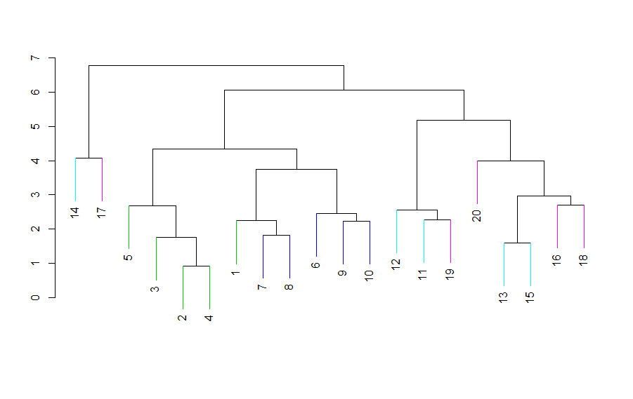
We apply SHC to . By gradually increasing the sparsity constraint, we obtain the sequence of the first 9 chosen variables , , , , , , }. The first three chosen features are noise features. As a result, the dendrogram generated from the first four chosen features (which is suggested by Witten and Tibshirani (2010)’s auto-selection method) gives mixed clusters (See Figure 1). The clustering result is still unsatisfactory even if seven variables are chosen (results not show here). Moreover, five noise features are selected before all the four clustering features are chosen.
3 Multi-rank sparse hierarchical clustering
To remedy this limitation of SHC, we propose the multi-rank sparse hierarchical clustering (MrSHC). Similar to SHC, MrSHC uses SPC as an important building block for feature selection, but MrSHC is different in the following aspects.
- •
MrSHC applies SPC directly to the original data . In comparison of applying SPC to a transformed dissimilarity matrix of size , this approach is more computationally efficient, more intuitive and proves to be effective given MrSHC’s superior performance in simulation studies and real data examples.
- •
Re-assign weight 1 to all the features with non-zero weights in sparse PCs. We call the re-assigned weights “indicator weights”. Indicator weights simply reflect whether features are selected, without further weighting on each feature, thus, facilitates the interpretation of the clustering results. Indicator weights also allow MrSHC to degenerate to classical hierarchical clustering if no sparsity constraint is applied.
- •
MrSHC identifies and recovers the clustering features using multi-rank sparse approximation through SPC. In other words, the clustering features are chosen according to the non-zero loadings in multiple sparse PCs. This allows MrSHC to adapt to features with more complex structures.
MrSHC is very different from the traditional approach where high-dimensional data are clustered based on the first few principal components. First, MrSHC applies SPC instead of traditional PCA to the data, also, MrSHC chooses the original features for clustering. The chosen features can be closely approximated by sparse low-rank approximations, in other words, they should have similar patterns of variations (e.g. if the features can be closely approximated by rank-1 approximation, then each of the features should have similar variation as the first PC). In clustering, similar patterns of variations usually represent information of clusters, and thus, the features chosen from MrSHC should contain key informations of clusters. This is confirmed by the simulated and real data examples in later sections.
We outline the MrSHC framework under the cases in Table 1.
| Case | ||
|---|---|---|
| 1 | Known | Known |
| 2 | Known | Unknown |
| 3 | Unknown | Unknown |
.
3.1 Case 1: Known and
Suppose the target number of clustering features and the appropriate rank of the SPC approximation are known. MrSHC applies SPC to and obtain the first sparse PCs. In MrSHC, a feature is considered selected if it has a non-zero loading in any of the sparse PCs. With an appropriately chosen sparsity constraint , we can get or approximately (say ) chosen features from the sparse PCs. MrSHC chooses using a bi-section approach presented in Algorithm 1.
We have seen in the simulations and real data examples that Algorithm 1 will finish in a few iterations.
Given and , a set of chosen features can be obtained from Algorithm 1. Then MrSHC simply generates a dendrogram (with any linkage of choice) based on the features in .
3.2 Case 2: Known , unknown
Suppose is known, but not . To choose , MrSHC first applies Algorithm 1 with increasing ranks , (different can be chosen; we choose here). Given rank , let denote the candidate feature set obtained from Algorithm 1. Different ranks will be compared through their corresponding . MrSHC assesses the quality of a feature set through the dendrogram generated from its features. To be more specific, a feature set is evaluated according to the following aspects.
- •
The number of well-separated clusters discovered from the dendrogram generated from . MrSHC uses a multi-layer pruning approach to obtain the well-separated clusters from a dendrogram. We introduce a “reference number of clusters" in the multi-layer pruning to facilitate later comparisons (described below).
- •
The degree of separation of the discovered clusters, which is evaluated by silhouette values (Rousseeuw, 1987).
Given the number of discovered clusters and the silhouette values, an iterative selection approach is proposed to choose the final rank .
Multi-layer pruning (MLP) prunes the dendrogram from the top to the bottom, with each split evaluated by the Gap statistics (Tibshirani et al., 2001). We introduce a “reference number of clusters” in MLP, which is both an “upper bound” and a “lower bound”. It is an upper bound of the number of clusters discovered in MLP. When is chosen properly, MLP will produce labels for clusters for most of the input dendrograms generated from , . This facilitates later comparisons since labels with different number of clusters are in general difficult to compare. It is also a lower bound of the number of clusters that are expected to be discovered. If less than clusters are discovered from a dendrogram according to MLP, such a dendrogram and its corresponding feature set are considered to be of low quality since key clusters may be missing. Therefore, such feature sets and their corresponding ranks are screened out and excluded from the later comparisons. Details of MLP are presented in Algorithm 2.
- •
If the chosen number of clusters is 1, set the current node as inactive;
- •
Otherwise, split the current node into two active leaf nodes.
- •
Number of leaf nodes (both active and inactive) is equal to .
- •
All the leaf nodes are inactive.
The reference number of clusters can be chosen based on subject area knowledge. If not specified, we set the default reference number of clusters to be , where is set as follows: apply MLP with to the dendrograms generated from , , then is the largest output number of leaf nodes from MLP. We have seen that in practice, a reliable can usually be found by applying MLP to , .
Suppose there are () left over dendrograms after screening out the ones with less than clusters. Let , and () denote their corresponding ranks, feature sets and labels (for clusters from MLP), respectively. Given and , the degree of separation of the corresponding clusters can be evaluated by the average silhouette value . High average silhouette values indicate well-separated clusters, and thus, are preferred. If two ranks lead to similar average silhouette values, the lower one is preferred since the feature set associated with the higher rank is more likely to contain noise variables. Therefore, among local minimums in (), the one with the highest rank is the least favourite, and thus, we remove such local minimums iteratively until the left-over are monotonically increasing or decreasing. Given monotonically increasing average silhouette values, the smallest rank after the largest increase in average silhouette value will be selected, since smaller ranks are preferred unless the increase in average silhouette value is large. On the other hand, if the average silhouette values are decreasing as rank increases, the smallest left-over rank will be selected. Details of this iterative selection approach are presented in Algorithm 3.
- •
increasing: the smallest rank after the biggest increase in the left-over .
- •
decreasing: the smallest left-over rank .
Once the chosen rank is obtained from Algorithm 3, MrSHC generates a dendrogram (with any linkage of choice) based on the features in .
We revisit the example in Section 2. Suppose is known, and we apply MrSHC with default reference number of clusters . The resulting with its corresponding rank contains the four true clustering features: , , and . The resulting dendrogram is presented in Figure 2. The four clusters are separated correctly.

3.3 Case 3: Unknown and
Suppose and are both unknown. MrSHC considers a list of target numbers of chosen features . For each of the candidate , MrSHC chooses its corresponding feature set () and average silhouette value as described in Section 3.2. Higher silhouette values are preferred, and at the mean time, smaller target numbers of features are preferred for the sake of interpretation and exclusion of noise features. Therefore, MrSHC uses a similar iterative approach as in Algorithm 3 to choose among (). Details of this iterative approach are presented in Algorithm 4.
- •
increasing: the smallest after the biggest increase in the left-over .
- •
decreasing: the smallest left-over rank .
Once the chosen is obtained from Algorithm 4, MrSHC generates a dendrogram (with any linkage of choice) based on the features in its corresponding .
Again, we revisit the example in Section 2. Suppose and are unknown, and we apply MrSHC with default reference number of clusters and the list of {}. MrSHC suggests and its corresponding feature set {, , }. Although is smaller than the true value , the four clusters can still be separated correctly (see Figure 3).

4 Simulation study
We conduct simulation studies to compare the quality of dendrograms and the accuracy of feature selection of the following methods: HC, SHC (with known/unknown ) and MrSHC (with known/unknown ). We show the results for all the methods with complete linkage. Similar results (not shown here) are obtained with other linkages.
4.1 Simulation I
We generate data sets with observations and features as follows. The observations are generated from three main underlying clusters C1, C2 and C3.
To be more specific, the clusters are determined by features as follows:
where and
We show the results for . Similar conclusions are obtained for other choices of , say .
We generate data sets and apply HC, SHC (with known/unknown ) and MrSHC (with known/unknown ) to each.
The quality of the resulting dendrograms is evaluated as follows. The dendrograms are cut at a level to obtain three clusters. The classification error rate (CER) is then used to assess clustering accuracy (Chipman and Tibshirani, 2006, see). We do this by comparing the resulting labels from three clusters against the underlying true labels (C1, C2, C3). Given two cluster partitions, the CER is the proportion of pairs of observations that are together in one partition and apart in the other. The formulas for the CER can be found in Chipman and Tibshirani (2006).
The accuracy of feature selection is evaluated by the recall rate (RR). Let be the set of indices corresponding to all the clustering features, and . The recall rate (RR) is calculated as follows:
where is an indicator function.
Table 2 presents the average CER, average RR, and the corresponding average . For SHC and MrSHC, the unknown is chosen automatically. HC gives the highest CER, while SHC achieves better accuracy due to the sparseness. MrSHC achieves the best accuracy among the three methods. When is known, SHC and MrSHC give very similar average RR. When is unknown, both methods give almost perfect RR, while MrSHC selects less features on average.
| HC | SHC | MrSHC | ||||||
|---|---|---|---|---|---|---|---|---|
| CER | CER | RR | CER | RR | ||||
| Known () | 0.202 | 500 | 0.047 | 0.926 | 50 | 0.009 | 0.995 | 50 |
| Unknown | 0.202 | 500 | 0.127 | 0.997 | 30.6 | 0.064 | 1.000 | 19.7 |
4.2 Simulation II
We generate data sets with observations and features, i.e. , where , . The observations are generated from four main underlying clusters C1, C2, C3 and C4. Let , () denote the cluster memberships. Then () is generated from for , and for .
A sketch of is presented in the table below:
| 1 | |||||||
|---|---|---|---|---|---|---|---|
| 2 | 0 | 0 | |||||
| 3 | 0 | 0 | |||||
| 4 | 0 | 0 | 0 | 0 |
We show the results for . Similar conclusions are obtained for other choices of .
Again, we generate data sets and apply HC, SHC (with known/unknown ) and MrSHC (with known/unknown ) to each. Table 3 presents the average CER, average RR, and the corresponding average . When is known, HC and MrSHC produce the highest and lowest average CER, respectively. MrSHC produces more accurate feature selection and clustering than SHC due to the smaller average CER and larger average RR. When is unknown, SHC produces the highest average CER with on average chosen features, while MrSHC achieves the smallest average CER with on average chosen features.
| HC | SHC | MrSHC | ||||||
|---|---|---|---|---|---|---|---|---|
| CER | CER | RR | CER | RR | ||||
| Known () | 0.172 | 500 | 0.129 | 0.875 | 50 | 0.041 | 0.977 | 50 |
| Unknown | 0.172 | 500 | 0.202 | 1.000 | 19.5 | 0.057 | 0.992 | 31.5 |
4.3 Computational times and complexity
We investigate the computational times of MrSHC and SHC. The HierarchicalSparseCluster function from the R-package sparcl is used to conduct SHC. MrSHC is implemented in R, where the SPC function from the R-package PMA is used to conduct the sparse PCA algorithm. We use default input parameters in MrSHC: the number of bootstrap samples , maximum rank , and default selection of the reference number of clusters . The average computing times for Simulation I & II are presented in Table 4.
| HC | SHC | MrSHC | ||||
| Simulation | I | II | I | II | I | II |
| Known () | 0.006 | 0.012 | 0.746 | 1.075 | 7.754 | 11.276 |
| Unknown | 0.006 | 0.012 | 10.496 | 15.518 | 73.254 | 103.752 |
When and are relatively small, SHC takes less time to compute. However, since the framework of MrSHC is embarrassingly parallel, parallel computing functions such as mcapply from the R-package multicore can be easily used to speed up the computation. Moreover, when and get larger, MrSHC will become less time consuming (observed with and , results not shown). This is because the computational complexities of MrSHC and SHC are and , respectively, and as a result, SHC will become more computationally demanding due to the term as and increase and .
5 Application to microarray data sets
Three microarray data sets (Alizadeh et al., 2000; Perou et al., 2000; van’t Veer et al., 2002) are considered. We apply HC, SHC, MrSHC, and HC using features with the highest marginal variance (HC-HMV) to each data set. Dendrograms are created using the complete linkage. The default reference number of clusters is used in MrSHC, and the default list of candidate (for both SHC and MrSHC) is .
5.0.1 Lymphoma data set in Dettling (2004)
The data set is provided by Dettling (2004). It contains 4026 gene expression levels (features) for 62 samples (observations). Three types of most prevalent adult lymphoid malignancies were studied: 42 cases of diffuse large B-cell lymphoma (DLBCL), 9 samples of follicular lymphoma (FL), and 11 observations of B-cell chronic lymphocytic leukemia (CLL). A specialized cDNA microarray was used to measure the gene expression levels. Following the pre-processing steps in Dudoit et al. (2002), the data set is pre-processed by first setting a thresholding window and then excluding genes with or . A logarithmic transformation and standardization are applied. Finally, a simple 5 nearest neighbor algorithm is employed to impute the missing values.
The dendrograms generated from HC, SHC, MrSHC and HC-HMV are shown in Figure 5. Colors are used to indicate the three tumor types. HC only misclassifies two red samples, while SHC gives mixed clusters with the automatically chosen . MrSHC chooses and uses rank , with only two blue samples misclassified into the green cluster (notice that the blue and green clusters are closer to each other). HC-HMV with mixes the blue and green clusters. Therefore, MrSHC achieves better clustering accuracy with a better chosen features using rank .

We further investigate the effect of the rank selection by the dendrograms in Figure . Figure (a) shows the dendrogram generated from MrSHC with , but . Figure (b) shows the dendrogram generated from SHC with . Both dendrograms suggest mixed clusters. This confirms that the rank selection can be crucial for better feature selection and clustering accuracy.

5.0.2 Breast cancer data set in Perou et al. (2000)
The data set was first published in Perou et al. (2000) and later analyzed in Witten and Tibshirani (2010). It contains 1753 gene expression levels (features) for 62 samples (observations) to profile surgical specimens of human breast tumors. Perou et al. (2000) categorized the 62 samples into four groups (clusters): basal-like, Erb-B2, normal breast-like, and ER+. Perou et al. (2000) suggested that the four underlying clusters could be explained by only 496 of the 1753 features, which was confirmed by Witten and Tibshirani (2010). Two misclassified samples were identified by Witten and Tibshirani (2010). The data set was pre-processed before being published. As such, there are no outliers in the data set.
Figure 6 shows the dendrograms generated from HC, SHC, MrSHC and HC-HMV. Colors are used to indicate the suggested four tumor groups. HC gives mixed clusters. SHC achieves better clustering – 5 misclassified samples, with the automatically chosen (similar results – features were automatically chosen and 5 samples are misclassfied – were obtained in Witten and Tibshirani (2010)). MrSHC misclassifies only 2 samples by using the automatically selected and rank . HC-HMV with gives mixed clusters. Although MrSHC chooses over higher ranks, it still provides better feature selection and more accurate clustering comparing to the other three methods.

5.0.3 Breast cancer data set in van’t Veer et al. (2002)
The data set was presented and analyzed in van’t Veer et al. (2002). It consists of 4751 gene expression levels for 77 primary breast tumor samples. A supervised classification technique was used in van’t Veer et al. (2002), revealing that only a subset of 70 out of the 4751 genes may help discriminating patients that have developed distant metastasis within five years.
Figure 7 shows the resulting dendrograms generated from HC, SHC, MrSHC and HC-HMV. HC misclassifies 6 samples. SHC achieves slightly better accuracy – 5 misclassified samples, with the automatically chosen . MrSHC with achieves the same accuracy with less () features. HC-HMV with features gives similar accuracy as MrSHC and SHC.

6 Conclusion
In this paper, we propose the multi-rank sparse hierarchical clustering (MrSHC), which automatically selects clustering features with higher rank considerations and produces the corresponding sparse hierarchical clustering. As demonstrated in simulation studies and real data examples, MrSHC gives superior feature selection and clustering performance comparing with the classical hierarchical clustering and the sparse hierarchical clustering proposed by Witten and Tibshirani (2010). For future research, we would like to endow MrSHC with the capability of dealing with data contamination: missing data and outliers.
References
References
- Alizadeh et al. (2000) Alizadeh, Ash A; Eisen, Michael B; Davis, R Eric; Ma, Chi; Lossos, Izidore S; Rosenwald, Andreas; Boldrick, Jennifer C; Sabet, Hajeer; Tran, Truc; Yu, Xin, and others, . Distinct types of diffuse large b-cell lymphoma identified by gene expression profiling. Nature, 403(6769):503–511, 2000.
- Chipman and Tibshirani (2006) Chipman, Hugh and Tibshirani, Robert. Hybrid hierarchical clustering with applications to microarray data. Biostatistics, 7(2):286–301, 2006.
- Dettling (2004) Dettling, Marcel. Bagboosting for tumor classification with gene expression data. Bioinformatics, 20(18):3583–3593, 2004.
- Dudoit et al. (2002) Dudoit, Sandrine; Fridlyand, Jane, and Speed, Terence P. Comparison of discrimination methods for the classification of tumors using gene expression data. Journal of the American statistical association, 97(457):77–87, 2002.
- Friedman and Meulman (2004) Friedman, Jerome H and Meulman, Jacqueline J. Clustering objects on subsets of attributes (with discussion). Journal of the Royal Statistical Society: Series B (Statistical Methodology), 66(4):815–849, 2004.
- Pan and Shen (2007) Pan, Wei and Shen, Xiaotong. Penalized model-based clustering with application to variable selection. The Journal of Machine Learning Research, 8:1145–1164, 2007.
- Perou et al. (2000) Perou, Charles M; Sørlie, Therese; Eisen, Michael B; van de Rijn, Matt; Jeffrey, Stefanie S; Rees, Christian A; Pollack, Jonathan R; Ross, Douglas T; Johnsen, Hilde; Akslen, Lars A, and others, . Molecular portraits of human breast tumours. Nature, 406(6797):747–752, 2000.
- Raftery and Dean (2006) Raftery, Adrian E and Dean, Nema. Variable selection for model-based clustering. Journal of the American Statistical Association, 101(473):168–178, 2006.
- Rousseeuw (1987) Rousseeuw, Peter J. Silhouettes: a graphical aid to the interpretation and validation of cluster analysis. Journal of computational and applied mathematics, 20:53–65, 1987.
- Sun et al. (2012) Sun, Wei; Wang, Junhui; Fang, Yixin, and others, . Regularized k-means clustering of high-dimensional data and its asymptotic consistency. Electronic Journal of Statistics, 6:148–167, 2012.
- Tibshirani et al. (2001) Tibshirani, Robert; Walther, Guenther, and Hastie, Trevor. Estimating the number of clusters in a data set via the gap statistic. Journal of the Royal Statistical Society: Series B (Statistical Methodology), 63(2):411–423, 2001.
- van’t Veer et al. (2002) van’t Veer, Laura J; Dai, Hongyue; Van De Vijver, Marc J; He, Yudong D; Hart, Augustinus AM; Mao, Mao; Peterse, Hans L; van der Kooy, Karin; Marton, Matthew J; Witteveen, Anke T, and others, . Gene expression profiling predicts clinical outcome of breast cancer. nature, 415(6871):530–536, 2002.
- Wang and Zhu (2008) Wang, Sijian and Zhu, Ji. Variable selection for model-based high-dimensional clustering and its application to microarray data. Biometrics, 64(2):440–448, 2008.
- Witten and Tibshirani (2010) Witten, Daniela M and Tibshirani, Robert. A framework for feature selection in clustering. Journal of the American Statistical Association, 105(490):713–726, 2010.
- Witten et al. (2009) Witten, Daniela M; Tibshirani, Robert, and Hastie, Trevor. A penalized matrix decomposition, with applications to sparse principal components and canonical correlation analysis. Biostatistics, 10(3):515–534, 2009.
- Xie et al. (2008) Xie, Benhuai; Pan, Wei, and Shen, Xiaotong. Penalized model-based clustering with cluster-specific diagonal covariance matrices and grouped variables. Electronic journal of statistics, 2:168, 2008.