Supporting Online Material to the manuscript: “Water isotope diffusion rates from the NorthGRIP ice core for the last 16,000 years - glaciological and paleoclimatic implications.”

In this section we show how we derive the numerical expressions for the diffusion length (Eq. (8) in main text (MT)). Starting from the differential equation for the diffusion length we have:

$$\frac{\mathrm{d}\sigma^{2}}{\mathrm{d}t}-2\,\dot{\varepsilon}_{z}\!\left(t\right)\sigma^{2}=2D\!\left(t\right).$$

(1)

We consider the vertical strain rate due to densification:

$$\dot{\varepsilon}_{z}\left(t\right)=\frac{-\partial\rho}{\,\,\,\partial t}\,\frac{\,1\,}{\,\rho\,}$$

(2)

By substituting $t$ with $\rho$ and combining Eq.(1), (2) we get:

$$\frac{\mathrm{d}\sigma^{2}}{\mathrm{d}\rho}+\frac{2\sigma^{2}}{\rho}=2{\left(\frac{\text{d}\rho}{\text{d}t}\right)}^{-1}D(\rho)$$

(3)

Multiplication of both sides of Eq.3 with the integrating factor

$$F(\rho)=e^{\int\frac{2}{\rho}\text{d}\rho}=\rho^{2},$$

(4)

gives:

$$\frac{\text{d}}{\text{d}t}\left(\rho^{2}\sigma^{2}\right)=2\rho^{2}{\left(\frac{\text{d}\rho}{\text{d}t}\right)}^{-1}D(\rho),$$

(5)

from which we get the result:

$$\sigma^{2}\left(\rho\right)=\frac{\,1\,}{\rho^{2}}\int_{\rho_{o}}^{\rho}2\rho^{2}{\left(\frac{\mathrm{d}\rho}{\mathrm{d}t}\right)}^{-1}\!D\!\left(\rho\right)\,\mathrm{d}\rho.$$

(6)

In a similar way for the ice diffusion length (Eq. (12) in the MT) we have:

$$\frac{\mathrm{d}\sigma^{2}}{\mathrm{d}t}-2\,\dot{\varepsilon}_{z}\!\left(t\right)\sigma^{2}=2D\!\left(t\right),$$

(7)

where the total thinning is given by:

$$\mathcal{S}\left(t^{\prime}\right)=e^{\int_{0}^{t^{\prime}}\dot{\varepsilon}_{z}\left(t\right)\mathrm{d}t}\kern 5.0pt.$$

(8)

We multiply both sides of Eq. (7) with the integrating factor

$$F(\rho)=e^{\int_{0}^{t^{\prime}}-2\dot{\varepsilon}_{z}\left(t\right)\mathrm{d}t},$$

(9)

which results in

$$\frac{\text{d}}{\text{d}t}\left[\sigma^{2}e^{\int_{0}^{t^{\prime}}-2\dot{\varepsilon}_{z}\left(t\right)\mathrm{d}t}\right]=2D(t)e^{\int_{0}^{t^{\prime}}-2\dot{\varepsilon}_{z}\left(t\right)\mathrm{d}t},$$

(10)

From this, we get the expression for the ice diffusion length

$$\sigma_{ice}^{2}\!\left(t^{\prime}\right)=S\!\left(t^{\prime}\right)^{2}\,\int_{0}^{t^{\prime}}2D_{ice}\!\left(t\right)S\!\left(t\right)^{-2}\,\mathrm{d}t.$$

(11)

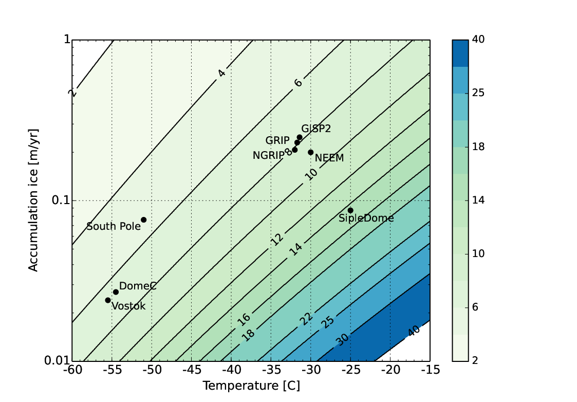
In this section we present an ensemble of implementations of the diffusion–densification model for various combinations of surface forcings that represent typical modern day conditions for a number of ice core sites on Greenland and Antarctica. The contours in the plot are generated by integration of Eq. (6) and expressed in m ice eq. The forcing for each ice core site is given in Table III and the results are shown in Fig. 2.

In order to estimate the diffusion length value from high resolution water isotope data we minimize the 2-norm $\|P_{s}-\hat{P}_{s}\|$ where $\hat{P}_{s}$ is an estimate of the power spectral density of a high resolution $\delta{}^{18}\mathrm{O}$ data section and $P_{s}$ is a model description of the power spectral density.

$\hat{P}_{s}$ is obtained by the use of the Burg’s spectral estimation method. The method fits an autoregressive model of order $\mu$ (AR-$\mu$) by minimizing the forward–backward prediction error filter (Hayes, 1996; Press et al., 2007; Andersen, 1974). For the theoretical model we have:

$$P_{s}=P_{\sigma}+{|\hat{\eta}\left(k\right)|}^{2},$$

(19)

where $P_{\sigma}=P_{0}\,{e}^{-k^{2}\sigma_{i}^{2}}$ is the effect of the firn diffusion process with squared diffusion length $\sigma^{2}$. Regarding the noise, we find red noise described by an AR-1 process with an autoregressive coefficient $q_{1}=0.15$ to provide a good description of the noise signal we observe. The spectrum of this signal is (Kay and Marple, 1981):

$$|\hat{\eta}(k)|^{2}=\frac{\sigma_{\eta}^{2}\Delta}{\left|1+q_{1}\exp{\left(-ik\Delta\right)}\right|^{2}}{},$$

(20)

where $\sigma_{\eta}^{2}$ is the variance of the noise. The angular frequency $k=2\pi f$ is in the range $f\in\left[0,\;\frac{1}{2\Delta}\right]$ defined by the Nyquist frequency and thus the sampling resolution $\Delta$. We vary the parameters $\sigma^{2},\,P_{0},$ and $\sigma_{\eta}^{2}$ of the spectral model in order to minimize the misfit between $P_{s}$ and $\hat{P}_{s}$ in a least squares sense.

As it can be seen in Fig. 3, it is the characterization of the full spectrum that yields information on $\sigma^{2}$. It is thus not necessary to specifically study the relative attenuation of individual spectral peaks as for example the annual signal. This approach allows for a study of the diffusion signal even after the spectral signature of the annual signal diminishes.

An interesting feature of the Burg estimation method is that the order $\mu$ of the AR filter affects the spectral resolution of $\hat{P}_{s}$ (Hayes, 1996; Press et al., 2007). Low $\mu$ values result in smoother spectra with inferior spectral resolution, while higher order spectra show better performance in resolving neighboring spectral peaks. This can be seen in the spectral estimates presented in Fig.3 where we plot spectral estimates with $\mu=30$ and $\mu=40$. As described above, the goal of the $\sigma^{2}$ estimation is to characterize the overall shape of the spectrum. As a result, relatively low values of $\mu$ produce smooth spectra of relatively low spectral resolution and can be adequate for the purpose of our application.

We look into both the influence of the value of $\mu$ on the $\sigma^{2}$ estimate by performing 41 power spectrum estimates with $\mu\in\left[40,80\right]$. Possible interferences of spectral features due to longer scale climate variability that could have an effect on the estimation of $\sigma^{2}$ are also investigated with this test. In Fig. 4 we show the mean value of the 41 spectral estimates before and after strain correction. The standard deviation of the estimated $\sigma$ for every depth is presented on the top subplot of the figure. It can be seen that on average the standard deviation is about 2 orders of magnitude lower than the absolute values of $\sqrt{\sigma^{2}}$ thus approximately in the 1% range. The low standard deviation of the 41 estimates suggests that a possible effect of spectral features due to low frequency climate variability is of second order. The same applies for the selection of the AR order $\mu$, in Burg’s spectral estimation.

Additional to the MEM order selection sensitivity test shown in section V, we investigate the precision and accuracy of the $\sigma^{2}$ estimation using synthetic data. We perform two tests which we describe below.

The layer thinning induced by the ice flow, impacts the diffusion length estimation mainly in two ways. First, due to the discrete sampling scheme as the diffusion length estimation moves towards the deeper parts of the core, a single sample averages more years of climate information. This effect is essentially taken care of by means of the discrete sampling correction described in section 4 of the MT. The term $\sigma_{dis}^{2}$ is constant with depth. However based on Eq. (20) of the MT one can see that the effective correction for discrete sampling scales with the total thinning function $S(z)$. In Fig. 9, we illustrate the effect of this correction with depth.

Second, the ice flow thinning will result in the diffusion length value decreasing with depth. With lower $\sigma^{2}$ values, a spectrum estimate up to the Nyquist frequency $1/2\Delta$ will contain a decreasing part of the noise signal ${|\hat{\eta}\left(k\right)|}^{2}$. After a certain depth, the sampling resolution is not high enough to resolve ${|\hat{\eta}\left(k\right)|}^{2}$. The result of this effect is that the estimation of the $P_{\sigma}$ signal requires an assumption about ${|\hat{\eta}\left(k\right)|}^{2}$ and thus it can limit the extend to which the diffusion technique can be applied to the deeper parts of the core.

In Fig. 7 we plot the expected diffusion length value assuming a simple case of constant temperature and accumulation rate at the surface and a certain ice layer thinning history. Then, based on this modeled diffusion length profile, in Fig. 8, we calculate six power spectral densities for $z=200,600,900,1200,1400\,\mathrm{and}\,1600\,\mathrm{m}$. For the spectral calculations we use 2 different sampling schemes, $\Delta_{1}=5\,\mathrm{cm\;and\;}\Delta_{2}=2.5\,\mathrm{cm}$. The plots illustrate the effect of the ice layer thinning as well as the sampling resolution on the shape of the power spectral density. As depth increases, a progressively smaller portion of the noise signal is resolved. Conclusively, for the deeper parts of the core where the ice layer thinning has reduced the diffusion length, a higher sampling resolution ($\Delta<2.5\,\mathrm{cm}$) is preferable for an even more accurate estimation of $P_{s}$ and subsequently $\sigma^{2}$ to be possible. For the NorthGRIP reconstruction we present here, we are able resolve the noise signal down to the depth of approximately 1450 m. For depths higher than 1450 m we make the simplest possible assumption that the noise level is equal to the average values we have observed in the Holocene section.

The accuracy of the ice flow model in inferring the ice thinning function has an influence on the uncertainty of our temperature reconstruction. The value of the diffusion length of a layer at depth $z$, estimated from the spectral properties of a set of $\delta{}^{18}\mathrm{O}$ data needs to be corrected for ice flow thinning. An inaccurately estimated thinning function affects the inferred values of $\sigma^{2}_{\text{firn}}$ in a linear way as we show in Eq. (13) and (20) of the MT. As far as the inferred temperatures are concerned, the ice thinning function impacts the slope of the signal, but has no influence on its variability.

In Fig. 10 we performed the temperature calculation using six different scenarios for the ice thinning function $S(z)$. We assume the simple scenario of a thinning function that varies linearly with depth and a value of $S(z=2100\;\text{m})$ equal to $0.22,0.24,0.26,0.28,0.30,0.32$. It is apparent that the change in temperature due to thinning function uncertainties can be significant. However this type of uncertainty only affects the slope of the temperature signal. So, unrealistic thinning function scenarios are relatively straightforward to rule out. Estimates of temperature from other proxies for any point of the record, can be useful in order to select a plausible scenario for the thinning function. This allows for a more accurate determination of slope of the temperature signal inferred by means of the firn diffusion method.

A direct consequence of this is that the method can potentially be useful in providing combined paleotemperature and glaciological information. In this study the unrealistically high temperature values we inferred for the Holocene climatic optimum pointed to possible inaccuracies of the ice thinning function used for the estimation. When fixing the temperature gradient between the Holocene optimum and present conditions to be approximately 3 K, we were able to propose a more likely scenario for the ice thinning function and hence the accumulation rate history. The temperature reconstruction using the proposed ice thinning function for NorthGRIP is presented in red color in Fig. 10.

Uncertainties related to the densification model affect the estimation of the diffusion length $\sigma^{2}_{\mathrm{firn}}$. Hereby we examine the influence of four parameters involved in the densification–diffusion model. We run a set of sensitivity experiments where the four firn densification parameters are perturbed in order to create a family of 1000 implementations of the diffusion-densification model for each experiment. For all the following sensitivity tests we also consider the standard deviation of the diffusion length spectral estimate as calculated in sections V and VI.

The first two parameters we consider are the surface and close–off densities $\rho_{0}$ and $\rho_{\mathrm{co}}$. We perform two sensitivity experiments where the values of $\rho_{0}$ and $\rho_{\mathrm{co}}$ are drawn from a Gaussian distribution with a defined mean and standard deviation (Table IV). For the close–off density a value of $804\;\pm 20\;\text{kgm}^{-3}\;(1\sigma)$ is used (Schwander et al., 1988; Jean-Baptiste et al., 1998; Johnsen et al., 2000). The range of values we choose for $\rho_{\text{co}}$ brackets within $2\sigma$ the more extreme estimates of $775\;\text{and}\;840\;\text{kgm}^{-3}$ shown in Scher and Zallen (1970) and Stauffer et al. (1985) respectively. For the surface density we use a value of $320\pm 40\;\text{kgm}^{-3}\;(1\sigma)$, based on modern observations of the firn column density at NothGRIP. Previous high resolution density observations by Albert and Shultz (2002) for Summit, Greenland indicate that the surface density can vary within $\pm 50\mathrm{kgm}^{-3}$ of its mean value. As a result, with a $1\sigma$ of $40\;\mathrm{kgm}^{-3}$ the Gaussian distribution of $\rho_{0}$ covers this range adequately in our sensitivity experiments.

Additionally, we include two parameters that describe the dependance of the densification rate to temperature. Based on Herron and Langway (1980)

$$\frac{\mathrm{d}\rho(z)}{\mathrm{d}t}=K(T)A^{\vartheta}\left(\rho_{\mathrm{ice}}-\rho\left(z\right)\right),$$

(21)

where $K(T)$ is a temperature dependent Arrhenius–type densification rate coefficient described by:

$$K(T)=11\exp\left(-\frac{10160}{RT}\right)\;\;\;\rho<550\;\mathrm{kgm}^{-3},$$

(22)

and

$$K(T)=575\exp\left(-\frac{21400}{RT}\right)\;\;\;\rho\geq 550\;\mathrm{kgm}^{-3}.$$

(23)

In order to perturb the model we use the term $K^{\prime}(t)$ in Eq. (21) where $K^{\prime}(T)=fK(T)$ and $f=1\pm 0.2\;(1\sigma)$. This results in a family of density profiles that are used for the diffusion length calculation. In Fig. 11 $1\sigma$ and $2\sigma$ intervals are illustrated together with firn density measurements from NorthGRIP.

The results of these sensitivity experiments are illustrated in Fig.12. Based on these results we conclude that using a fixed value for the surface and close–off densities is a plausible approach. The combined uncertainty of the $\rho_{o}$ and $\rho_{\text{co}}$ parameters is in the order of 1 K and thus the temperature history we infer is consistent over a wide range of densification parameter values. Combining all densification parameters the uncertainty of the estimation is equal to $\pm 2.5\,\mathrm{K}\,(1\sigma)$. Combining this in a Gaussian sense with the spectral estimation uncertainty from section VI we get a total of $\pm 2.7\,\mathrm{K}\,(1\sigma)$.

References

- Albert and Shultz (2002) Albert, M. R., Shultz, E. F., May 2002. Snow and firn properties and air-snow transport processes at summit, greenland. Atmospheric Environment 36 (15-16), 2789–2797.
- Andersen (1974) Andersen, N., 1974. Calculation of filter coefficients for maximum entropy spectral analysis. Geophysics 39 (1), 69–72.
- Blicks et al. (1966) Blicks, H., Dengel, O., Riehl, N., 1966. Diffusion von protonen (tritonen) in reinen und dotierten eis-einkristallen. Physik Der Kondensiterten Materie 4 (5), 375–381.
- Dahl Jensen et al. (1998) Dahl Jensen, D., Mosegaard, K., Gundestrup, N., Clow, G. D., Johnsen, S. J., Hansen, A. W., Balling, N., Oct. 1998. Past temperatures directly from the Greenland ice sheet. Science 282 (5387), 268–271.
- Delibaltas et al. (1966) Delibaltas, P., Dengel, O., Helmreich, D., Riehl, N., Simon, H., 1966. Diffusion von in eis-einkristallen. Physik Der Kondensiterten Materie 5 (3), 166–170.
- Hall and Pruppacher (1976) Hall, W. D., Pruppacher, H. R., 1976. Survival of ice particles falling from cirrus clouds in subsaturated air. Journal of the Atmospheric Sciences 33 (10), 1995–2006.
- Hayes (1996) Hayes, M. H., 1996. Statistical digital signal processing and modeling. John Wiley & Sons.
- Herron and Langway (1980) Herron, M. M., Langway, C., 1980. Firn densification - an empirical-model. Journal Of Glaciology 25 (93), 373–385.
- Itagaki (1967) Itagaki, K., Feb. 1967. Self-diffusion in single crystal ice. J. Phys. Soc. Jpn. 22 (2), 427–431.
- Jean-Baptiste et al. (1998) Jean-Baptiste, P., Jouzel, J., Stievenard, M., Ciais, P., May 1998. Experimental determination of the diffusion rate of deuterated water vapor in ice and application to the stable isotopes smoothing of ice cores. Earth And Planetary Science Letters 158 (1-2), 81–90.
- Johnsen et al. (2000) Johnsen, S. J., Clausen, H. B., Cuffey, K. M., Hoffmann, G., Schwander, J., Creyts, T., 2000. Diffusion of stable isotopes in polar firn and ice. the isotope effect in firn diffusion. In: Hondoh, T. (Ed.), Physics of Ice Core Records. Hokkaido University Press, Sapporo, pp. 121–140.
- Johnsen et al. (1995) Johnsen, S. J., Dahl Jensen, D., Dansgaard, W., Gundestrup, N., Nov. 1995. Greenland paleotemperatures derived from GRIP bore hole temperature and ice core isotope profiles. Tellus Series B-Chemical And Physical Meteorology 47 (5), 624–629.
- Johnsen et al. (2001) Johnsen, S. J., DahlJensen, D., Gundestrup, N., Steffensen, J. P., Clausen, H. B., Miller, H., Masson-Delmotte, V., Sveinbjornsdottir, A. E., White, J., 2001. Oxygen isotope and palaeotemperature records from six greenland ice-core stations: Camp Century, Dye-3, GRIP, GISP2, Renland and NorthGRIP. Journal Of Quaternary Science 16 (4), 299–307.
- Kay and Marple (1981) Kay, S. M., Marple, S. L., 1981. Spectrum analysis - a modern perspective. Proceedings Of The Ieee 69 (11), 1380–1419.
- Majoube (1971) Majoube, M., 1971. Fractionation in o-18 between ice and water vapor. Journal De Chimie Physique Et De Physico-Chimie Biologique 68 (4), 625–&.
- Merlivat (1978) Merlivat, L., 1978. Molecular diffusivities of , , and gases. Journal of Chemical Physics 69 (6), 2864–2871.
- Merlivat and Nief (1967) Merlivat, L., Nief, G., 1967. Fractionnement isotopique lors des changements detat solide-vapeur et liquide-vapeur de leau a des temperatures inferieures a 0 degrees c. Tellus 19 (1), 122–127.
- Murphy and Koop (2005) Murphy, D. M., Koop, T., Apr. 2005. Review of the vapour pressures of ice and supercooled water for atmospheric applications. Quarterly Journal Of The Royal Meteorological Society 131 (608), 1539–1565.
- Percival (1993) Percival, D. B., 1993. Spectral analysis for physical applications. Cambridge University Press.
- Press et al. (2007) Press, W. H., Teukolsky, S. A., Vetterling, W. T., Flannery, B. P., August 2007. Numerical Recipes: The Art of Scientific Computing. Cambridge University Press.
- Ramseier (1967) Ramseier, R. O., 1967. Self-diffusion of tritium in natural and synthetic ice monocrystals. Journal Of Applied Physics 38 (6), 2553–2556.
- Scher and Zallen (1970) Scher, H., Zallen, R., 1970. Critical density in percolation processes. Journal of Chemical Physics 53 (9), 3759–3761.
- Schwander et al. (1988) Schwander, J., Stauffer, B., Sigg, A., 1988. Air mixing in firn and the age of air at pore close-off. Annals Of Glaciology 10, 141–145.
- Stauffer et al. (1985) Stauffer, B., Schwander, J., H., O., 1985. Enclosure of air during metamorphosis of dry firn to ice. Annals of Glaciology 6, 108–112.
- Vinther et al. (2009) Vinther, B. M., Buchardt, S. L., Clausen, H. B., Dahl-Jensen, D., Johnsen, S. J., Fisher, D. A., Koerner, R. M., Raynaud, D., Lipenkov, V., Andersen, K. K., Blunier, T., Rasmussen, S. O., Steffensen, J. P., Svensson, A. M., 2009. Holocene thinning of the greenland ice sheet. Nature 461 (7262), 385–388.