interaction in finite volume and the resonance
Abstract
We evaluate energy levels of the system in the channel in finite volume using chiral unitary theory. We use these energy levels to obtain phase shifts, and then obtain the mass and its decay width. We investigate their dependence on the pion mass and compare this with Lattice QCD calculations. We also compare our method with the standard Lüscher approach, and solve the inverse problem to obtain the phase shifts from these “synthetic” lattice data.
pacs
12.38.Gc, 12.39.Fe, 13.75.LbI Introduction
Lattice QCD is developing very fast in these years. One can use this method to evaluate the discrete energy levels of the finite box, and then reconstruct phase shifts of the decay products in the continuum. To do this, one usually uses the Lüscher’s approach [1, 2], which has a higher accuracy and consistency with the decay channels of the hadrons, and so it is widely used in lattice studies [3, 4]. These discrete energy levels can not be directly measured in the experiments. However, in Ref. [5] the authors proposed one method to estimate them through an effective approach whose parameters are obtained by fitting the experimental data.
This method has been applied in Ref. [6] to obtain finite volume results from the Jülich model for meson baryon interaction, and in Ref. [7] to study the interaction of the and systems where the resonance is dynamically generated from the interaction of these channels [8, 9, 10, 11]; the case of the resonance in the -wave channel is studied in Ref. [12]; the case of resonance in the and channels in finite volume is studied in Ref. [13]. An extension of the approach of Ref. [5] to the case of interaction of unstable particles is studied in Ref. [14]. We also use it to study the interaction of two pions in the channel in finite volume [15].
In the present work we shall study the interaction in the channel in finite volume. This meson has been measured very well in the experiments and we can use the chiral unitary model to well describe it. Recently several Lattice groups also studied it and evaluated the relevant discrete energy levels using the Lüscher’s approach [16, 17, 19]. Again we note that these energy levels can not be directly measured in the experiments, so one needs to make extra efforts in order to compare these energy levels with the experimental data of the meson. Lattice theorists usually transform these energy levels into the phase shifts, and then calculate the physical quantities of the meson. Accordingly, one can do the opposite process [5], and this is what we shall study in this paper, i.e., in this paper we shall follow the approach of Ref. [5], and inversely transform the experimental data of meson into “synthetic” energy levels. To do this we need to use the chiral unitary model to study the interaction in the channel in finite volume. To make a complete analysis, we shall also use these “synthetic” data to calculate the phase shifts and then calculate the physical quantities for the meson. We shall refer to the results of Refs. [16, 17, 18] for comparison along the paper. We shall also compare our method with the standard Lüscher approach, and solve the inverse problem and obtain the phase shifts from these “synthetic” lattice data.
This paper is organized as follows. In Sec. II we study the scattering in the region using the chiral unitary model both in infinite space and in finite volume. Then in Sec. III we use these formulae to evaluate energy levels and phase shifts. The pion mass dependence of these results is studied in Sec. IV where we also study their comparison with the Lattice data. We compare our method with the standard Lüscher approach in Sec. V, and solve the inverse problem to obtain phase shifts from these “synthetic” lattice data in Sec. VI. Finally we show some concluding remarks in Sec. VII.
II The Chiral Unitary Approach In Infinite and Finite Box
The scattering amplitude in -wave has been studied in Refs. [20, 21] by using the chiral unitary model. In this paper we shall follow the same approach and use the following Bethe-Salpeter equation in their on-shell factorized form [20, 21, 22, 23] (for a quantitative study of off-shell effects in this context, see, e.g., Ref. [24]):
| (1) |
Here we only consider the channel, but the and channels may also be important. In Ref. [25], the (892) is studied with the coupled channels , and . The coupling of the (892) to is the dominance, but some smaller, although not negligible couplings to and are also found. The couplings by themselves do not give a measure of the relevance of the channel, because if the mass of the channel is far away from the pole, the relevance would be much smaller for a same coupling. Furthermore, in such a case, the effect of these channels and other missing channels can be absorbed in the study with one channel by changing the subtraction constants, and the energy dependence of the potential a bit, which is explicitly done in our model. Indeed, the fit to the data with just the channel is very good, as found in Ref. [20] and shown below. Moreover, the elimination of one channel in terms of an effective potential for another channel in the content of lattice QCD analysis has been shown to be a valid and useful tool in Ref. [26].
The relevant -matrix for the scattering has been studied in Refs. [20, 27, 21]:
| (2) |
where is the bare mass, is the decay constant, and is the coupling for a vector meson to two pseudoscalar mesons. We note that this potential is a bit different from the one used in Ref. [21], where the factor is absorbed into their -function so that does not depend on the momentum. The -function for the two-meson (-) propagator having masses and is defined as
| (3) |
where is the four-momentum of the external meson-meson system. There are many methods to regularize this loop-function. In Ref. [21] the authors use the cut-off method, but in this paper we shall use the dimensional regularization which is more convenient when studying the interaction in finite volume. We note that these two methods are equivalent up to certain energy level range, as proved in Ref. [23]. The dimensional regularization result is
| (4) |
where , is the on-shell momentum of the particles, is a regularization scale and is a subtraction constant. In this paper we shall work in the center-of-mass frame, where the energy of the system is . The regularization parameters are chosen to be
| (5) | |||||
| (6) |
The two parameters and are taken from Ref. [21]:
| (7) | |||||
| (8) |
but the parameter is a bit different from the one used in Ref. [21], because we are using the dimensional regularization other than the cut-off method used in Ref. [21]. To fix , we use the experimental data of the -wave phase shifts, which are related to the through:
| (9) |
where is the center-of-mass momentum. We use the experimental data of Refs. [30, 29], and evaluate . The fitting results are shown in Fig. 1, where is fitted to be:
| (10) |
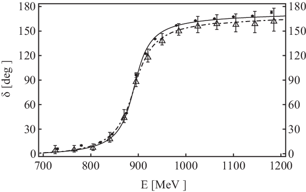
All the above formulae are defined in the infinite space. To study the meson in the finite volume, we simply change the -function of dimensional regularization (Eq. (4)) by the one which is defined in the finite box of side [28, 7], i.e., we simply change the integration over momenta by a sum over the discrete values of the momenta allowed by the periodic conditions in the box. We denote the latter one by , and it can be obtained through:
| (11) |
In this equation the discrete momenta in the sum are given by and the function is
| (12) |
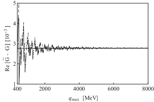
where . We show the real part of in Fig. 2 as a function of , where is fixed to be 2.5 and to be MeV. Its convergence is good when is larger than 3000 MeV. However, we shall still make an average of this quantity for smaller values of in order to save the computational time [28, 7].
III The Energy Levels in the Chiral Unitary Approach
To calculate the energy levels of the scattering amplitude in -wave, we need to find the poles of the matrix, which are just solutions of the following equation
| (13) |
Here is defined in the finite volume and can be obtained through Eq. (11). From this equation we can clearly see that the energy levels for -wave scattering are functions of the cubic box size , as well as the pion mass . In the following sections we shall study their dependence on these variables. In this section we study the volume dependence and in the next section we shall study the pion mass dependence. We note again that our procedures follow closely the method used in Refs. [28, 7, 15, 12, 13, 14].

In Fig. 3 we show the energy levels as functions of the cubic box size , which are obtained after performing an average for different values between 1200 MeV and 2000 MeV. Actually, the results for different values are almost the same. In this figure we have used the dimensional regularization, Eq. (4), to calculate Eq. (3) and then calculate of Eq. (11), while we can also use the cut-off method to calculate Eq. (3):
| (14) |
which can be inserted into Eq. (11) and then calculate . The energy levels can be similarly calculated and the results are shown in Fig. 4. We note that the cutoff used in Eq. (14), denoted as , is different from used in Eq. (11). We choose to be 724.70 MeV following Ref. [21]. It is significantly larger than the discrete momentum MeV when is around 2.0 .

The phase shift can be extracted from these energy levels. To do this we follow the procedure used in Ref. [5], and use Eq. (9) to calculate the -wave phase shifts, where the scattering amplitudes are obtained using the energy levels shown in Fig. (3):
| (15) |
Here we have used Eq. (13), i.e., . Although these procedures can be done for all energy levels, the lowest energy level should be the best one, because we are using the chiral unitary approach which is an effective theory for low energies. Accordingly, we use the lowest energy level to evaluate phase shifts, and the result is shown in Fig. 5. For comparison, we also show the phase shifts evaluated using the second and the third energy levels.


Using the phase shift we can fit the physical quantities for the meson, and evaluate , and . We note that is the mass we obtained, i.e., one of our outputs; while is the bare mass, i.e., one of our inputs. To do that, we use the following two equations in Refs. [15, 26] to extract the properties:
| (16) |
We note that the factor in the second equation is our normalization, while in Ref. [18] the authors use . The results from fitting the phase shifts calculated using the lowest energy level are
| (17) |
In these results the theoretical uncertainties are estimated following Ref. [15], where we assume that the uncertainties of the three parameters , and in Eq. (2) are all about 4%. The uncertainties of the energy levels and phase shifts are shown in Fig. 6. Particularly, the uncertainty of phase shifts is quite large around . However, the fitted results shown in Eq. (17) have moderate and acceptable uncertainties, suggesting our method is “stable” (see also the discussions in Sec. V).
Similarly, we can fit the second and the third energy levels. We find that the results do not change much: the results from fitting the phase shifts calculated using both the first and the second energy levels are (overlapped points are counted just once):
| (18) |
and the results from fitting the phase shifts calculated using all the three energy levels are (overlapped points are counted just once):
| (19) |


IV Dependence on the Pion Mass
As we know, due to the computer limitation, the Lattice QCD calculations usually use a non-physical pion mass. Therefore, in this section, we also use non-physical pion masses to study the mass and decay width of the meson, in order to compare with the Lattice QCD result. We define to be the physical mass, and now is a free parameter. We change it from to . At the same time other parameters can also change with . We follow the same approach of Refs. [15, 31, 32, 33, 34], where the variation of as a function of is
| (20) |
with MeV. The coupling is related to [35, 36, 37, 38], as , valid to leading order, consequently, we keep unchanged. The kaon mass can also change with the pion mass , and we use the following relation [39]:
| (21) |
where , and . We note that the Lattice calculations also use non-physical kaon masses [16, 17], but all these values are not much different from the physical one. Accordingly, in this paper we shall first keep it unchanged, then use the kaon mass in Eq. (21), and finally use the same values of as the Lattice ones [16, 17] in order to compare our results with theirs. On the other hand, the bare mass, in Eq. (2), provides the link of the theory to a genuine component of the meson, not related to the component, and we assume it to be independent.
To calculate the energy levels we follow the same procedures which have been used in the previous section. The result is shown in Fig. 7 where we have used (left), (middle) and (right). The solid curves are obtained using the physical kaon mass , and the dotted curves are obtained using the non-physical kaon mass evaluated using Eq. (21). We can see that the results obtained using these different kaon masses do not differ much. Here, we note that the -coordinate is expressed in units of , not .


These energy levels can be used to calculate the phase shifts again following our previous procedures. The results are shown in Fig. 8, where again we have used (left), (middle) and (right). The solid curves are obtained using the physical kaon mass , and the dashed curves are obtained using the non-physical kaon mass evaluated using Eq. (21). We note that the dashed curve on the right of Fig. 8 vanishes, because the sum of and non-physical kaon mass is already above the threshold.
Now we can compare our results with the Lattice results of Refs. [16, 17], where MeV and MeV are used in Ref. [16], and MeV and MeV are used in Ref. [17]. We show their comparisons in Fig. 9 and Tables 1 and 2, where and are on the lowest and the second energy levels, and and are extracted from and , respectively. We find that the energy levels and the extracted phase shifts are similar, and so our results compare favorably with those lattice results obtained in Refs. [16, 17]. Again the theoretical errors are obtained by assuming that the uncertainties of the three parameters , and in Eq. (2) are about 4%. We also show more points in Table 3 which may be useful.
| Our Results | ||
|---|---|---|
| Lattice Results |
| Our Results | ||||
|---|---|---|---|---|
| Lattice Results |
Finally, we use Eq.(16) to fit the phase shifts obtained using the lowest energy level, and obtain the mass (left), the coupling constant (middle) and the decay width (right), which are shown in Fig. 10 as functions of . We can see that the results of obtained using the physical kaon mass and non-physical kaon masses in Eq. (21) are very similar, while the results of and are not so similar. This may be because the phase spaces differ much, although the kaon masses do not differ much. We also note that when using Eq. (21), the physical kaon mass can not be reached at the physical pion mass . Therefore, the dashed curves and the solid curves are not connected. Again we can compare our results with the lattice results in Ref. [18], where , and . Their results are MeV and , which change to MeV and in our normalization after taking into account the factor . These results are in agreement, within uncertainties, with our result MeV and .


To be complete, we also show the results calculated by fitting the phase shifts obtained using the three lowest energy levels of Fig. 11. The solid curves are obtained using the first (lowest) energy level, the dotdashed curves are obtained using both the first and the second energy levels, and the dashed curves are obtained using all the three lowest energy levels. We find that these results are almost the same.
V Comparison of our results with the standard Lüscher’s approach
To make our analysis complete, we compare our results with the Lattice results obtained using the standard Lüscher’s approach [5]. To do this, we follow the same approach of Refs. [15, 31, 32, 33, 34]: we use as input the energy levels which we have calculated in Sec. III and Sec. IV using our -functions (Eqs. (4) and (11)), but evaluate phase shifts using both our method and the Lüscher’s -function.


The function of Eq. (12) can be written as
| (22) |
In the standard Lüscher’s approach only the first term of this equation is kept. We use the following two sets of energy levels: a) the lowest energy level shown in Fig. 3, where MeV and MeV are used; and b) the lowest energy level shown in the right panel of Fig. 9, where MeV and MeV are used [17]. The obtained phase shifts are shown in Fig. 12, where the dashed curves are the phase shift evaluated using the standard Lscher’s approach and the solid curves are our results. These phase shifts can be similarly used to fit the physical quantities:
| (23) | |||||
Comparing these two figures, we clearly see that the Lscher’s results and our results are quite similar in case (b) when nonphysical pion and kaon masses are used. This confirms the validity of the standard Lüscher’s approach in the real simulation. There are some differences in case (a) when the physical pion and kaon masses are used, but still both results are consistent with each other within uncertainties, considering the uncertainties related to phase shifts are quite large, as shown in the right panel of Fig. 6.
We note that this discrepancy is partly caused by hidden systematics in different approaches. Moreover, the result at higher energy is obtained using a smaller volume, which could cause sizable finite volume effects (see also discussions in Refs. [2, 15]). Accordingly, we would like to suggest Lattice theorists to pay attention to this effect when they extract the physical information using the Lattice data calculated in a (too) small box, for example, if they want to use the physical pion mass but still the computational power is limited. For completeness, we try to find where these differences come from by adding the second, the third and the fourth terms of Eq. (22) to the first standard Lüscher’s term. The results for physical pion and kaon masses, are shown in Fig. 13, and the results for MeV and MeV, are shown in Fig. 14. These results suggest that the relativistic corrections can be well taken into account by simply adding either the third or the fourth terms of Eq. (22).


VI THE INVERSE PROBLEM OF GETTING PHASE SHIFT FROM LATTICE DATA
In this section we study the inverse process of getting phase shifts from Lattice Data using two energy levels and a parametrized potential. This has also been done in Refs. [5, 7, 12, 13, 15, 14], showing this method is rather efficient. To do this we assume that the first and second energy levels shown in Fig. 3 are “Lattice” inputs, or “synthetic” data. We shall use them to inversely evaluate the -matrix and then calculate phase shifts. At the same time we shall give these “lattice data” some error bars which can be used to evaluate the uncertainties of the phase shifts.
Our procedures follow Refs. [5, 7, 12, 13, 15, 14]. We take five energies from the first level and five more from the second one (we note that their volumes are also different), and associate to them an error of 10 MeV. Then we use the following function which accounts for a CDD pole [40] to do the one-channel fitting:
| (24) |
where , and are three free parameters which we shall fit with the “Lattice” data shown in Fig. 3. The results are shown Fig. 15 where the energy levels are calculated from all the possible sets of parameters having . Here is the best fitting we obtained, where the three parameters are:
| (25) |
we find that errors in the phase shift are large at small energies, but they become smaller as the energy increases.
As mentioned in Ref. [5] the result of this inverse analysis does not depend on which cut off, or subtraction constant one uses in the analysis, as far as one uses the same ones to induce from the lattice data and then later on to get phase shifts in the infinite volume from Eq. (1). The method proves to be practical and efficient.


VII Conclusion
In this paper we use the efficient strategy proposed in Ref. [5] to obtain phase shifts, and thus the meson properties from energy levels obtained in lattice calculations. To do this we studied the interaction in -wave in a finite box using the chiral unitary approach which has been very successful to provide phase shifts in infinite space. We evaluated energy levels which are functions of the cubic box size and the pion mass . Then we use these energy levels to obtain phase shifts. Finally we use these phase shifts to fit the physical quantities for the meson: , , . To compare our results with the Lattice QCD calculations, we also used non-physical pion masses and redid the same calculations. We note that other parameters can also change with , and we have considered these effects. The comparison of our results with the Lattice QCD results are shown in Table 1 and Table 2, where we can see our results compare favorably with those lattice results obtained in Refs. [16, 17]. We note that in these calculations we have estimated the theoretical uncertainties.
To make our analysis complete, we compare our results with the Lattice results obtained using the standard Lüscher’s approach. We find that the Lscher’s results and our results are quite similar for the resonance when the non-physical pion and kaon masses, MeV and MeV, are used. There are some differences when the physical pion and kaon masses are used, although both results are still consistent with each other within uncertainties. This discrepancy is partly caused by hidden systematics in different approaches. Moreover, the result at large energy are obtained using a small volume, and could cause sizable finite volume effects. Accordingly, we would like to suggest Lattice theorists to pay attention to this effect when they extract the physical information using the Lattice data calculated in a (too) small box, for example, if they want to use the physical pion mass but still the computational power is limited. Our analyses also suggest that the relativistic corrections can be well taken into account by simply adding either the third or the fourth term of Eq. (22). We also studied the inverse process of getting phase shifts from our “synthetic¡¯¡¯ lattice data using two energy levels and a parametrized potential.
VIII Acknowlegement
We thank Eulogio Oset for suggesting this problem and valuable help, and Bao-Xi Sun, Chu-Wen Xiao and Xiu-Lei Ren for useful discussion and information. We also than Zhi-Hui Guo for useful discussion and information about Ref. [25], and we have started to study the (892) resonance in finite volume with coupled channels , and . This work is supported by the National Natural Science Foundation of China under Grant No.11205011, 11475015, 11375024 and 11375023, and the Fundamental Research Funds for the Central Universities.
References
- [1] M. Lüscher, Commun. Math. Phys. 105 (1986) 153.
- [2] M. Lüscher, Nucl. Phys. B 354 (1991) 531.
- [3] V. Bernard, M. Lage, U. G. Meissner and A. Rusetsky, JHEP 0808 (2008) 024.
- [4] V. Bernard, M. Lage, U.-G. Meissner and A. Rusetsky, JHEP 1101 (2011) 019.
- [5] M. Doring, U. -G. Meissner, E. Oset and A. Rusetsky, Eur. Phys. J. A 47, 139 (2011).
- [6] M. Doring, J. Haidenbauer, U. -G. Meissner, A. Rusetsky, Eur. Phys. J. A 47, 163 (2011).
- [7] A. Martinez Torres, L. R. Dai, C. Koren, D. Jido and E. Oset, Phys. Rev. D 85, 014027 (2012).
- [8] E. E. Kolomeitsev, M. F. M. Lutz, Phys. Lett. B582, 39-48 (2004).
- [9] J. Hofmann, M. F. M. Lutz, Nucl. Phys. A733, 142-152 (2004).
- [10] F. -K. Guo, P. -N. Shen, H. -C. Chiang, R. -G. Ping, B. -S. Zou, Phys. Lett. B641, 278-285 (2006).
- [11] D. Gamermann, E. Oset, D. Strottman, M. J. Vicente Vacas, Phys. Rev. D76, 074016 (2007).
- [12] M. Doring, U. G. Meissner, JHEP 1201, 009 (2012).
- [13] J. -J. Xie and E. Oset, Eur. Phys. J. A 48, 146 (2012).
- [14] L. Roca and E. Oset, Phys. Rev. D 85, 054507 (2012).
- [15] Hua-Xing Chen and E. Oset, Phys. Rev. D 87,016014 2013
- [16] Ziwen Fu and Kan Fu, Phys. Rev. D 86, 094507 (2012).
- [17] C. B. Lang, and Leskovec Luka and Mohler Daniel and Prelovsek Sasa, Phys. Rev. D 86, 054508 (2012).
- [18] S. Prelovsek, L. Leskovec, C. B. Lang and D. Mohler, Phys. Rev. D 88, no. 5, 054508 (2013).
- [19] J. J. Dudek et al. [Hadron Spectrum Collaboration], Phys. Rev. Lett. 113, no. 18, 182001 (2014).
- [20] J. A. Oller and E. Oset, Phys. Rev. D 60, 074023 (1999).
- [21] C. W. Xiao, F. Aceti, and M. Bayar, Eur. Phys. J. A 49, 22 (2011).
- [22] J. A. Oller and E. Oset, Nucl. Phys. A 620, 438 (1997) [Erratum-ibid. A 652, 407 (1999)].
- [23] J. A. Oller and U. G. Meissner, Phys. Lett. B 500, 263 (2001).
- [24] M. Altenbuchinger and L. S. Geng, Phys. Rev. D 89, no. 5, 054008 (2014).
- [25] Z. H. Guo and J. A. Oller, Phys. Rev. D 84, 034005 (2011).
- [26] C. B. Lang, D. Mohler, S. Prelovsek and M. Vidmar, Phys. Rev. D 84, 054503 (2011).
- [27] J. A. Oller, E. Oset and J. E. Palomar, Phys. Rev. D 63, 114009 (2001).
- [28] M. Doring, J. Haidenbauer, U.-G. Meisssner, A. Rusetsky, Eur. Phys. J. A 47, 163 (2011).
- [29] P. Estabrooks, R. K. Carnegie, A. D. Martin, W. M. Dunwoodie, T. A. Lasinski and D. W. G. S. Leith, Nucl. Phys. B 133, 490 (1978).
- [30] R. Mercer, P. Antich, A. Callahan, C. Y. Chien, B. Cox, R. Carson, D. Denegri and L. Ettlinger et al., Nucl. Phys. B 32, 381 (1971).
- [31] P. Boucaud et al. [ETM Collaboration], Phys. Lett. B 650, 304 (2007).
- [32] S. R. Beane, T. C. Luu, K. Orginos, A. Parreno, M. J. Savage, A. Torok and A. Walker-Loud, Phys. Rev. D 77, 014505 (2008).
- [33] J. Noaki, S. Aoki, T. W. Chiu, H. Fukaya, S. Hashimoto, T. H. Hsieh, T. Kaneko and H. Matsufuru et al., PoS LATTICE 2008, 107 (2008).
- [34] J. R. Pelaez and G. Rios, Phys. Rev. D 82, 114002 (2010).
- [35] J. J. Sakurai, Currents and mesons (University of Chicago Press, Chicago Il 1969).
- [36] M. Bando, T. Kugo and K. Yamawaki, Phys. Rept. 164, 217 (1988).
- [37] G. Ecker, J. Gasser, H. Leutwyler, A. Pich and E. de Rafael, Phys. Lett. B 223, 425 (1989).
- [38] Y. Zhou, X. L. Ren, H. X. Chen and L. S. Geng, Phys. Rev. D 90, no. 1, 014020 (2014).
- [39] X. -L. Ren, L. S. Geng, J. Martin Camalich, J. Meng and H. Toki, JHEP 1212, 073 (2012).
- [40] L. Castillejo, R. H. Dalitz and F. J. Dyson, Phys. Rev. 101, 453 (1956).