The voter model chordal interface in two dimensions
Abstract
Consider the voter model on a box of side length (in the triangular lattice) with boundary votes fixed forever as type 0 or type 1 on two different halves of the boundary. Motivated by analogous questions in percolation, we study several geometric objects at stationarity, as . One is the interface between the (large – i.e., boundary connected) 0-cluster and 1-cluster. Another is the set of large “coalescing classes” determined by the coalescing walk process dual to the voter model.
1 Introduction
In this section we motivate our study of the (two-dimensional) voter model and its dual coalescing walks through their connection with a number of percolation models. In Section 2, we report on numerical results for the dimension of a natural “chordal interface” of the voter model. In Section 3 we give rigorous (and a few numerical) results on the large coalescing classes for coalescing walks (where vertices and in a box are in the same class if their walks coalesce before hitting the boundary). In the appendix, more details about our numerical results are provided.
Among the most important breakthroughs in statistical physics and probability in the last two decades is the work by Schramm and coauthors [7, 13, 14] and Smirnov [15, 16, 17] identifying (or conjecturing) members of the Schramm-Loewner Evolution family of random curves as the scaling limits of various random walks and interfaces in two-dimensional spin systems. In particular Smirnov [15, 16] (see also Camia and Newman’s paper [2]) has shown that the scaling limit of critical site-percolation on the triangular lattice is SLE6. To give a rough description of one version of this statement, take a rhombic box (containing vertices) in the triangular lattice in two dimensions. Label the sides clockwise starting from the southwest corner as . A percolation configuration on is an element of defined as follows. Fix the vertices in and to have value 0 (or black or closed) and those in and to be 1 (or red or open). In the interior , set each vertex to be (independently) 0 or 1, with probability each – see Figure .

There exists a unique simple path of length from the southwest corner following edges in the dual hexagonal lattice to the opposite corner that keeps black/closed vertices on the left and red/open vertices on the right. is often referred to as the exploration path; we will also call it the chordal interface. As the law of , after rescaling, converges weakly to a probability measure on continuous paths that is the law of chordal SLE6 [2, 15] in a rhombic domain. One can use this to prove (see [12, Prop. 2]) that , where
| (1) |
In general for we have that if and only if
| (2) |
Note that uniquely determines the path . One can therefore ask about the limiting behavior of when the configurations are generated by some other process (i.e., not i.i.d. critical site percolation) in the interior . In the case of the Ising model (where the states at two sites are not independent) at the critical temperature, Smirnov [17] has identified that the limiting probability measure is instead chordal SLE3. We are interested in the limiting behavior of when the law of the configuration is the stationary distribution of the voter model (or related models) on .
1.1 The voter model
In this section we define our primary model of interest, on as described above, with boundary states set as 0 on one pair of adjacent sides and 1 on the other pair, while the law of the interior states is the stationary measure for the voter model on , as follows.
Each has its own independent Poisson clock (a Poisson process ) of rate 1. When the clock of a vertex rings we update the state of by choosing one of its six neighbors uniformly at random and adopting the state of the chosen neighbor. Note that the neighbor may be one of the vertices in the boundary whose state is fixed. Defined this way, is an irreducible Markov process with finite state space , and therefore it has a unique invariant distribution. We will write for a random configuration sampled from this invariant distribution.
The process admits a well-known graphical representation (due to T.E. Harris [6]) which we now review. For each , we draw a positive half line (representing time) in the third dimension, and on it we mark the times of Poisson clock rings of that vertex. Each mark on a time line represents a state update event which also has an arrow from to the uniformly chosen neighbor whose state is adopted. The lines of the boundary vertices have arrow marks to them, but not from them, as those states are fixed.
Fix an initial configuration . To determine the state of a vertex at time we start at height/time on the time line corresponding to and follow it down until we reach height/time 0 or we encounter an outgoing arrow (whichever comes first) at height . If we meet an outgoing arrow we follow it to the time line of a neighboring vertex and proceed as before, following this time line down from height until reaching height/time 0 or an outgoing arrow. We stop this procedure when we reach a boundary vertex or height 0 on some time line. Thus from any and the path followed corresponds to a continuous time nearest neighbor simple random walk on stopped upon reaching a boundary vertex or height 0. In either case the state at the terminal vertex is known and we set .
Such a system of “state genealogy walks” from all the vertices at time following backward in time is a dual model and is distributed as a system of coalescing simple symmetric continuous time random walks on the triangular lattice – see for example [5]. Since is finite, if is large enough all the walks starting then will with high probability hit the boundary before reaching height 0. Indeed, if we continue the time lines and Poisson clocks below height 0 (and do not terminate the walks at height 0) then almost surely from any height there will be a random height at which the walks started from all vertices at height will have reached boundary vertices. What happens on the time lines below height does not affect since the states of the boundary vertices are fixed for all time. This is equivalent to saying that the voter model itself reaches stationarity by a random finite time (distributed as ).
Therefore to sample from it is enough to follow a system of coalescing continuous time simple random walks from each vertex of until they hit a boundary vertex , and set , i.e. if , and otherwise. One could instead sample from by setting for every (so the state space would become ) and simulating the voter model dynamics until there is no vertex with state 2.
Figure shows a simulation of with , obtained by simulating coalescing random walks from each vertex in the interior, until each one has reached the boundary.

1.2 Harmonic percolation and related models
The duality discussed in the previous section tells us that (we drop the superscript when there is no ambiguity) is the probability that a simple random walk started at first hits the boundary at a 1-site. In other words, the one-dimensional distributions of our voter model on are equal to those of a model we would like to call harmonic percolation. This is a model under which the states are independent of each other, and as we have already suggested, is equal to the probability that a simple random walk started from first hits the boundary at a 1-site (i.e., in ). Harmonic percolation on an infinite strip of thickness coincides with an independent percolation model called gradient percolation [9, 10, 11]. In the case of gradient percolation the probability of a site being open changes linearly from one boundary where it is 0 to the other boundary where it is 1. Thus the function is harmonic inside the strip (with specified boundary conditions). The difference between the voter and harmonic percolation models arises from the fact that the walks in the former are coalescing, whereas in the latter they are independent. To be more explicit, coalescence in the voter model leads to non-zero correlations as in the following simple lemma.
Lemma 1.1.
For any , and any in the interior of ,
| (3) |
Proof.
Fix , and , and let and denote the elements of with fixed states 0 and 1 respectively. Let and be two independent random walks starting from and respectively. Let be the first time that and meet each other. Let for all times and define
| (4) |
so that and are coalescing walks started from and respectively.
Let and denote the respective hitting times of the boundary, and note that . Then
| (5) | ||||
This proves the result for . A similar coupling argument can be made for any number of walkers starting from vertices (choosing the lower indexed random walker to continue when any two meet), establishing the claim. ∎
For any , if and are distance at least from each other and the boundary then there exist and such that for and all , while
where and are times when the difference random walk started at first hits the origin and the boundary of the box respectively, and the last equality follows from Proposition 6.4.3 of [8]. Then (5) implies that the correlation between the votes at and goes to zero as per the following.
Lemma 1.2.
Let , and and be distance at least from each other and the boundary . Then as .
One can consider i.i.d. percolation, harmonic percolation, and the stationary voter model on as special cases of a general 2-parameter family of models as follows. Start a continuous-time walker from each site. Each walker initially wears a hat. Two walkers wearing hats coalesce when they meet, and instantly become a single walker wearing a hat. Walkers not wearing hats do not coalesce with any other walkers. In addition a Poisson clock is assigned to each walker. When such a clock rings, the walker takes a random walk step, but before doing so removes her coalescence hat with probability . If a walker wearing a hat steps into a site with another walker with a hat on, the walker that just made its step becomes part of the coalescence set of the walker that was already at the site. Upon hitting a boundary site, with probability a walker (and its entire coalescence set) is assigned the vote of the boundary vertex it hit, and otherwise (i.e., with probability ) its entire coalescence set attains an independently and uniformly chosen vote. Varying the boundary and coalescence noise parameters and between 0 and 1 allows us to interpolate between the four corner models: the voter model ; harmonic percolation ; i.i.d. percolation ; and the case corresponds to a model we would like to call cow (coalescing walk) percolation.
2 Interface length
Recall that denotes the length of the interface. Since this path is a nearest neighbor simple path, there exist such that almost surely. We conjecture that
| (6) |
for some . In the case of critical i.i.d. percolation, (6) holds with which is also the Hausdorff dimension of the limiting law (i.e., of SLE6, see [1]).
For gradient percolation on an infinite strip, the interface curve between the occupied cluster and empty cluster is a.s. unique and has expected length approximately , where is the horizontal length of the piece of strip in which we measure boundary length [9, Proposition 11]. So, for any , for all sufficiently large , if we take a piece of strip which is long (and thick), the expected length of the interface curve satisfies . For any , with probability going to 1 with , the curve stays in the central band (around the central line where ) of width [9, Theorem 6]. Thus, as , unless we appropriately zoom in around the central line, we expect to see the rescaled interface curve converge to a straight line in the center. Since the harmonic function inside a rhombic area with our boundary condition looks almost linear along the diagonal that connects the middle corner of the 1 valued boundary to the middle corner of the 0 valued boundary (or indeed along any parallel line), we expect that the interface curve for harmonic percolation inside our rhombus should scale to a straight line as well.
Writing for some function which makes the equality true we have that
| (7) |
Computing the average interface curve length from independent realizations of we obtain the following estimators for based on (7)
| (8) | ||||
| (9) |
We say that an estimator (more precisely a family of estimators ) is a consistent estimator of some quantity if
| (10) |
It is easy to show that is a consistent estimator of if and only if as (i.e., if and only if ), while is a consistent estimator for if and only if as . Thus both estimators are consistent if is slowly varying at .
If we are willing to assume that the random interface length in a box of size satisfies , where , then it is natural to consider the ordinary least squares estimator for the slope coefficient of the simple linear regression model
| (11) |
where are interface lengths on boxes of side lengths , and the are random variables with mean 0. Note that is constant under this assumption.
The results from independent simulations of computing the average lengths of the interface curve and estimates (with ) appear in Table . For ordinary percolation and harmonic percolation the values are known (or expected) to be and , so for these models (with ) appears to do best. For the voter model the value of is about 1.46.
| voter | 1.4427 | 1.4581 | 1.4633 | 1.5947 | 1.5767 | 1.5638 | 1.5536 | 1.4586 (s.e. 0.0012) |
| cow. | 1.4809 | 1.4876 | 1.4953 | 1.6689 | 1.6454 | 1.6279 | 1.6146 | 1.4878 (s.e. 0.0019) |
| harm. | 1.4229 | 1.4221 | 1.4290 | 1.6254 | 1.6001 | 1.5803 | 1.5652 | 1.4264 (s.e. 0.0006) |
| perc. | 1.7401 | 1.7463 | 1.7505 | 1.8492 | 1.8355 | 1.8256 | 1.8181 | 1.7458 (s.e. 0.0019) |
3 The sizes of coalescing classes and related questions
The interface curve cannot pass through any connected cluster of common votes. The difference between the voter and harmonic percolation models is that the states are determined by coalescing random walks rather than independent random walks (started at each site). If the coalescing classes in the voter model are negligible as , both in terms of size and the correlation between votes in different classes, then perhaps some kind of rescaling argument would allow one to compare the voter model to the harmonic percolation model. One expects that the rescaled interface curve for harmonic percolation on converges to a straight line (Pierre Nolin has proved this on the strip [9]), so one might expect the same to be true for the voter model, if the coalescing classes are indeed negligible as .
Clustering behaviour for the 2-dimensional voter model has been well studied in the probability literature (see e.g. [4]), but (as far as we know) not in the current setting of a finite domain with unflinching boundary. As a small step in the direction of understanding the correlation between votes in different classes, let us verify that any two sites and are less likely to share a common vote (than they otherwise would be) if they are not in the same coalescing class. Fix and start coalescing walks from every site in . The walks define an equivalence relation on in the sense that if and only if the walks started from and coalesce before hitting the boundary. Let denote the (random) equivalence class of . Let and . Then and
as claimed. On the other hand, as we have seen earlier, if and are distance at least apart then and as , with being bounded away from zero as if and are also at least distance from the boundary.
We are hereafter interested in the behavior of the expected size of the class of the centre of the rhombus , which we will for convenience take to be the origin (if is not odd we consider the centre/origin to be any one of the closest vertices to the centre) and the expected size of the largest class as , where
| (12) |
where some tie-breaking rule is used to choose , if necessary. In particular, we ask what proportion of all vertices in the box are in the largest class, as ? Since , we are interested in . Figure shows a single realization of the 5 largest classes for .

The following is our main rigorous result, which shows that coalescing classses have (on average) small (but only logarithmically small) volume compared to the whole box. We note that the lower bound can be improved slightly with a little more effort.
Theorem 3.1.
There are constants and in , such that
| (13) |
Proof.
First note that to have centered at the origin and to have the smaller rhombi used in the proof to be consistent with the lattice we need to be such that is divisible by 12, and then for rhombi of fractional side lengths such as we should use instead of . For notational convenience we will ignore these issues, but we note though that the same arguments would in any case work with trivial but messy modifications.
For both the upper and lower bounds in (13) we will use the fact that, for ,
| (14) |
To verify the lower bound, let be independent continuous-time (with jump rate 1), nearest-neighbor random walks on the triangular lattice, with respective starting points . For , let , and denote the meeting times and boundary hitting times respectively. Then (14) with can be written as
| (15) |
By Lemma below there is positive constant such that for each ,
| (16) |
Combining (15) and (16) we obtain
| (17) |
for another positive constant , which verifies the lower bound in (13).
To establish the upper bound, note that for any the difference walk is also a simple symmetric random walk started at but with jump rate 2. Let and be the first hitting times of the origin and the boundary by the difference walk , and let be the first time hits the origin. Then
| (18) |
Using Theorem 6.4.3 of [8] on the summation, (18) is bounded above by
| (19) |
Next, we split the sum into dyadic annuli (all but finitely many of which contain no vertices). Since has been defined via the number of vertices on the boundary (so only for integer ), we let denote the rhombic box centered at the origin in and let denote the (possibly empty) intersection of () with the triangular lattice. Then the first term in (19) is equal to
Therefore
| (20) |
Markov’s inequality gives for any , so
| (21) |
It follows that
| (22) | ||||
Choose to get the claimed upper bound. ∎
Lemma 3.2.
Fix some small . There exists , such that for all ,
| (23) |
Proof.
The triangular lattice is constructed from 3 families of parallel lines (or “directions”), denoted by , with each vertex being at the intersection of 3 such lines (one from each family), and having 6 nearest neighbors corresponding to moving “up” or “down” in any one of these directions. We define a system of two dependent discrete-time random walks and on the triangular lattice in the following way: and ; for each toss a fair coin to decide which of or makes an i.i.d. uniformly chosen nearest-neighbor step on the triangular lattice (while the other does not move). Let , , and be the corresponding meeting and boundary hitting times for and . Since has the same law as the jump process of and the event in (23) depends only on the relative sizes of the hitting times, we have
| (24) |
Now we focus on the discrete time random walks and . For , let denote the set of ordered partitions of into three (possibly empty) sets. For , let denote the direction of the step taken by (one of) the pair at time . For let be the event that for each and , , i.e., that steps in direction are taken at times in etc. Conditioning on we can rewrite the probability above as follows
| (25) |
Let and denote the difference and sum walks starting at , defined by and , and let and , and and be the hitting times of the origin and the boundary by the difference and sum walks respectively. Since
| (26) |
we have
| (27) |
A similar statement holds for . Thus we have
| (28) |
Therefore (25) can be continued as follows
| (29) | ||||
where the last equality follows from the fact that the sum and difference walks are conditionally independent given (e.g., if we know that the sum walk makes a positive step in a specific direction, the difference walk is still equally likely to make either a positive or negative step in that direction).
Let . Truncating the infinite sum and using Lemma below we have
| (30) | ||||
where denotes the (discrete) time a one-dimensional simple symmetric random walk started at first hits or . Summarizing from (25) until this point, and continuing we have
| (31) |
where the last inequality follows from Lemma below.
Let be the size of the range of a one-dimensional discrete-time random walk (started at ) up to time . Then
| (32) |
According to Theorem 2 of [3], for any sequence diverging to
| (33) |
where . Letting , and , (32) and (33) yield (for ) that for large (and ),
| (34) |
Similarly, with and , (32) and (33) yield (for ) that for large (and ),
| (35) |
According to Theorem 6.4.3 of [8] the term for can be bounded uniformly from below and above by and for some positive constants and and large enough. Inserting this estimate, (34) and (35) into (31) verifies that there exists a constant such that for all , uniformly in ,
| (36) |
as required. ∎
Lemma 3.3.
With the definitions of , , , and as in the proof of Lemma , for any and we have
| (37) | ||||
| (38) |
Proof.
To verify the first claim, first recall the definition of after (24). For each we construct a two-dimensional random walk on the triangular lattice (started at , with and steps along the three directions in respectively) from a one-dimensional random walk of steps in the following way: let the one-dimensional walk be with each ; designate the first steps to be in direction “”, the next steps to be in direction “”, and the final steps to be in direction “”; construct the two-dimensional random walk starting at by picking steps from each group according to the partition (preserving the order of steps within each of the groups). If the one-dimensional walk started at the origin stays confined to the interval , then the first steps, next steps and next steps have displacements from their respective starting points at most , , and respectively and the two-dimensional walk started at stays confined to . Therefore we have for that
| (39) |
This verifies the first claim.
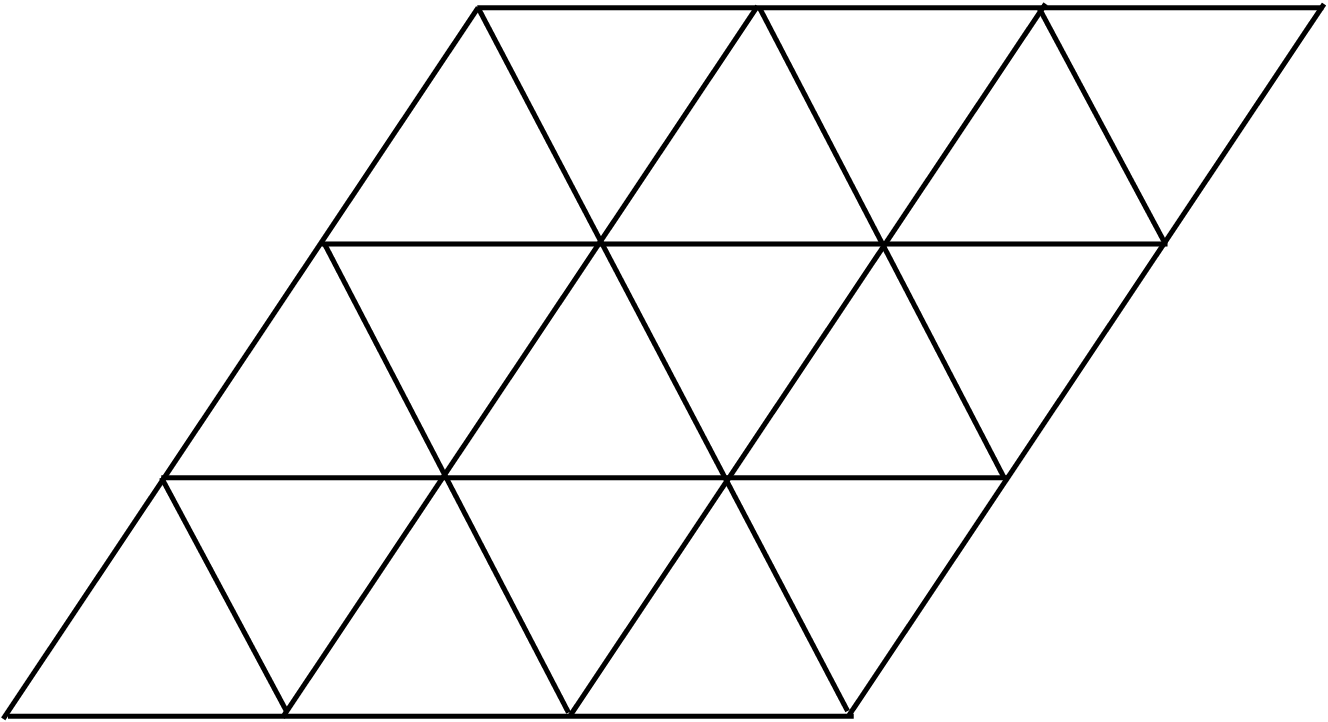

For the second claim, we consider two one-dimensional random walks, and , that are the following “projections” of the two-dimensional discrete-time (difference) random walk starting at onto the lines parallel to the two sides of the rhombic box . Under the linear transformation depicted in Figure “projections” are simply standard orthogonal projections onto the two coordinate axes. Thus, the walk makes no step when steps in the direction , makes a step -1 when the increment of is either or , and +1 when the increment of is either or . Similarly does not move when steps in the direction , while it makes an increment -1 (resp., +1) when the increment of is or (resp., or ). Let be the hitting time of by , and be the number of steps made by by the time makes steps. Then we have
| (40) | ||||
∎
Theorem and the discussion preceding it suggest the following conjecture.
Conjecture 3.4.
The interface curve of the voter model in converges to a straight line as .
Theorem also provides us with a useful test of the quality of our numerical estimation techniques (which are of course for finite ). Having established that and with , we estimated the exponents from simulation data with estimators as in (8),(9), and (11) giving
| (41) | ||||
| (42) |
Thus, again the estimators are closest to the true value.
Figure suggests that the (largest) coalescing classes are rather disconnected and sparse, which poses a potential problem for a rescaling argument like that mentioned at the beginning of Section . This is because the coalescing classes will not scale to single points if their diameters are with non-vanishing probability. It is an open problem to prove that for some , . This would imply that with positive probability there are coalescing classes with diameter at least . A very large proportion of our simulated curves cut through in the sense that the interface curve has sites belonging to on both sides. The proportion increases from 0.9819 for the boxes of size 128, to 0.9985 for the boxes of size 1024. Thus, the connected clusters/subsets (containing ) of coalescing classes , may be better candidates to use in rescaling arguments as the interface curve has to go around them. Assuming that and , we obtain the estimates and .
Another piece of information that may support Conjecture is the displacement of the curve from its conjectured diagonal limit, . Assuming that , we obtain the estimate .
Acknowledgements
MH thanks David Wilson for helpful discussions at the initial stages of this project. MH and YM thank Raghu Varadhan, Federico Camia, and Pierre Nolin for helpful discussions and the Centre for eResearch at U. Auckland for providing the computing resources and support. The work of MH and YM was supported by an FRDF grant from U. Auckland. The work of CMN was supported in part by US NSF grants OISE-0730136 and DMS-1007524.
References
- [1] V. Beffara. The dimension of the SLE curves. Ann. Probab. 36:1421–1452, (2008).
- [2] F. Camia and C.M. Newman. Critical percolation exploration path and : a proof of convergence. Probab. Theory Related Fields 139:473–519, (2007).
- [3] X. Chen. Moderate and small deviations for the ranges of one-dimensional random walks. J. Theor. Probab. 19:721-739, (2006).
- [4] J.T. Cox and D. Griffeath. Diffusive clustering in the two-dimensional voter model. Ann. Probab. 14:347–370, (1986).
- [5] D. Griffeath. Additive and Cancellative Interacting Particle Systems. Lecture Notes in Math. 724. Springer, Berlin (1979).
- [6] T.E. Harris. Additive set-valued Markov processes and graphical methods. Ann. Probab. 6: 355–378, (1978).
- [7] G.F. Lawler, O. Schramm, and W. Werner. Conformal invariance of planar loop-erased random walks and uniform spanning trees. Ann. Probab. 32:939–995, (2004).
- [8] G.F. Lawler and V. Limic. Random Walk: A Modern Introduction. Cambridge University Press, (2010).
- [9] P. Nolin. Critical exponents of planar gradient percolation. Ann. Probab. 36:1748–1776, (2008).
- [10] P. Nolin. SLE(6) and the geometry of diffusion fronts. arXiv:0912.3770
- [11] P. Nolin. Inhomogeneity and universality: off-critical behavior of interfaces. arXiv:0907.1495
- [12] P. Nolin and W. Werner. Asymmetry of near-critical percolation interfaces. J. Amer. Math. Soc. 22:797–819, (2009).
- [13] O. Schramm. Scaling limits of loop-erased random walks and uniform spanning trees. Israel J. Math. 118:221–288, (2000).
- [14] O. Schramm and S. Sheffield. Harmonic explorer and its convergence to . Ann. Probab. 33:2127–2148, (2005).
- [15] S. Smirnov. Critical percolation in the plane: conformal invariance, Cardy’s formula, scaling limits. C. R. Acad. Sci. Paris Sér. I Math. 333:239-244, (2001).
- [16] S. Smirnov. Critical percolation in the plane. arXiv:0909.4499 (2001).
- [17] S. Smirnov. Towards conformal invariance of 2D lattice models. Proc. Int. Congr. Math. 2:1421-1451, (2006).
4 Appendix
As indicated earlier, each of our estimates is based on 10000 independent simulations of the voter model for each value of being considered. Although the simulations had a finite time horizon, in all cases all coalescing walks eventually reached the boundary. All simulations were conducted in C++ and all statistical analyses and plots were performed in R. The data is available on request, but at approximately 600GB, may be difficult to transfer.
Note also that all of our simulations actually took place on boxes of side length , so our estimators were actually
| (43) | ||||
| (44) |
Similarly our ordinary least squares estimator is in fact an estimator for the slope coefficient of the simple linear regression model
| (45) |
where are interface lengths on boxes of side lengths , and the are random variables with mean 0. This does not change the consistency properties of the estimators, and e.g. results in an estimate differing in only the fourth decimal place when we are dividing by (instead of ).
4.1 The size of coalescing classes
Since the and estimators are defined straightforwardly and have already been discussed somewhat at the end of Section , let us turn our attention here to the regression estimators for the class sizes. Assume that the assumptions prior to (11) hold for and with exponents and respectively, so that e.g.
| (46) |
We obtain an estimate of by fitting the simple linear model . Fitting this linear model in R we obtain the following output:
Call:  lm(formula = log(cluster_large) ~ log(L))

Residuals:
     Min       1Q   Median       3Q      Max
-0.93002 -0.22984 -0.02386  0.20920  1.34982

Coefficients:
             Estimate Std. Error t value Pr(>|t|)
(Intercept) -1.726828   0.028139  -61.37   <2e-16 ***
log(L)       1.897190   0.004374  433.72   <2e-16 ***

Residual standard error: 0.3201 on 12998 degrees of freedom
Multiple R-squared: 0.9354,     Adjusted R-squared: 0.9354
F-statistic: 1.881e+05 on 1 and 12998 DF,  p-value: < 2.2e-16
Figure and the standard diagnostic tests suggests that the model fits very well. However, the estimate for is more than 20 standard errors from the known (from Theorem ) true value of , so this estimator seems to be doing a poor job of estimating the true limiting behaviour in . We believe that this is caused by our inability to simulate the model for very large .


For the coalescing class of the center, the linear regression estimator fits less well and gives an estimate of (see also Figure ).
Call:  lm(formula = log(cluster_origin) ~ log(L))

Residuals:
    Min      1Q  Median      3Q     Max
-4.5422 -0.4825  0.0914  0.5688  2.1029

Coefficients:
            Estimate Std. Error t value Pr(>|t|)
(Intercept) -2.09387    0.06964  -30.07   <2e-16 ***
log(L)       1.84149    0.01083  170.10   <2e-16 ***

Residual standard error: 0.7923 on 12998 degrees of freedom
Multiple R-squared:  0.69,      Adjusted R-squared:  0.69
F-statistic: 2.894e+04 on 1 and 12998 DF,  p-value: < 2.2e-16


4.2 Connected clusters of a coalescing class
Recall from the end of Section that for each configuration of a voter model in , denotes the connected subset (containing ) of the coalescing class of . Letting denote a largest such connected subset and assume
Recalling the discussion around (9), we obtain the following estimates, which indicate that this estimator converges more slowly with increasing than the corresponding estimator for the expected curve length exponent.
| 128 | 256 | 512 | |
|---|---|---|---|
| 1.69253 | 1.71810 | 1.74051 | |
| 1.47049 | 1.49151 | 1.54791 |
4.3 Maximum displacement of the curve from the diagonal
Recall the last paragraph of Section . Under the assumption that we have the following estimates for .
| 128 | 256 | 512 | |
|---|---|---|---|
| 0.96847 | 0.97545 | 0.97068 |
Fitting a simple linear model to the data gives a very similar estimate of 0.9689 (which is about 18 standard errors away from 1) as per the following.
Residuals:
     Min       1Q   Median       3Q      Max
-1.11443 -0.17013  0.01359  0.18474  0.59812

Coefficients:
             Estimate Std. Error t value Pr(>|t|)
(Intercept) -1.090206   0.009573  -113.9   <2e-16 ***
log(Lvec)    0.968864   0.001611   601.4   <2e-16 ***

Residual standard error: 0.2497 on 39998 degrees of freedom
Multiple R-squared: 0.9004,     Adjusted R-squared: 0.9004
F-statistic: 3.617e+05 on 1 and 39998 DF,  p-value: < 2.2e-16