Designing Path Planning Algorithms for
Mobile Anchor towards Range-Free Localization

Localization of wireless sensors with high degree of accuracy is required for many wireless sensor networks (WSNs) applications, such as security and surveillance, object tracking, detecting accurate location of a target etc. To meet this purpose, many sensor localization schemes [2, 4, 5, 10, 15, 17, 18, 19] have been proposed for WSNs. These schemes can be viewed as range-based or range-free. In range-based schemes, the sensor locations are calculated using distance and/or angle information among sensors by ranging hardware. On the other hand, connectivity constraints such as hop-count, anchor beacons etc are used in range-free schemes. Usually range-based schemes are more accurate than range-free schemes. But range estimation techniques in range-based schemes are erroneous as well as costly due to requirement of special hardware, which encouraged researcher to design range-free schemes for sensor localization. A number of static anchors are needed in the localization schemes like [2, 4, 5, 15, 19] which uses static anchors. To minimize the number of static anchors, localization schemes [10, 17, 18] using mobile anchor are proposed. One mobile anchor with a suitable path planning is equivalent to many static anchors, which localizes whole network. By using mobile anchor, we can save large number of anchors with deployment cost in the expense of the mobility of the mobile anchor. So, path planning of the mobile anchor has become an important issue in the area of localization. There are few proposed movement strategies which localizes sensors using some basic techniques like trilateration [16], which causes large localization error. Our aim is to propose a movement strategy such that we can use existing range-free localization schemes which yields better accuracy.

In this paper we have proposed path planning schemes for the mobile anchor where localization is done using localization scheme proposed by Lee et al.[10].We have proposed two different movement strategies for two different assumptions. One movement strategy is proposed on the assumption that the network is connected. The anchor localizes every sensor of the network with connectivity guided movement. The other movement strategy is proposed to localize sensors over a bounded rectangular region where the anchor has to cover the whole rectangle to ensure localization of all sensors. In this strategy, only boundary information is used to localize all the sensors irrespective of deployment and underlying network topology.

Path planning algorithms set path for mobile anchor along which it moves in the network while localization process goes on. First we look at a brief overview of the existing range free localization schemes which provides good accuracy and can be used for localization. Ssu et al. proposed a localization scheme in [17] where the sensor’s position is estimated as the intersection of perpendicular bisector of two calculated chords. However this scheme suffers from short chord length problem. Xiao et al.[18] improved over that scheme using pre-arrival and post-departure points along with the beacon points to localize a sensor. Later Lee et al. used beacon distance more effectively as another geometric constraint and proposed a more accurate localization scheme in [10].

We can view the path planning problem in two different ways depending on the knowledge of the area of sensor deployment and the underlying topology formed by the sensors. Topology-based path planning, can be viewed as a graph traversal problem. Sensors have information about their neighbors which they send to the mobile anchor for determining the path. Li et al. proposed two algorithms named breadth first and backtracking greedy algorithms in [11]. Mitton et al. in [12] proposed a depth first traversal scheme by the mobile anchor to localize the sensors. Both these works need range estimations. Kim et al. proposed a path planning in [8] for randomly deployed sensors using trilateration method for localization. An already localized sensor becomes a reference point to help other sensors to find their position which reduces path length but localization error may propagate. Chang et al. proposed another path planning algorithm of the mobile anchor in [3] where localization have been done using the scheme proposed by Galstyan et al. in [1] and mobile sensor calculates its trajectory by moving around already localized sensors. Our aim is to propose a path planning algorithm which can decide its trajectory without using any range estimation in a connected network. Using connectivity of the network, we discover neighbors of a sensor as well as localize it by the scheme [10] using our proposed path planning algorithm.

The other way of viewing the path planning problem is to cover a rectangular area by the mobile anchor where all the sensors are deployed. $Scan$, $Doublescan$ and $Hilbert$ schemes are proposed by Koutsonikolas et al. in [9]. They used the localization scheme proposed in [13]. Scan covers the whole area uniformly where the mobile anchor travels in line segments along $x$-axis (or $y$-axis) keeping a fixed distance between two line segments. In $Doublescan$, anchor moves along both $x$-axis and $y$-axis, which improves localization accuracy in the expense of traveled distance. $Hilbert$ reduces both error and path length with compare to the other two. Huang et al. proposed two path planning schemes namely $Circles$ and S-curves in [7]. Simulation results show that these two schemes produce better results than those discussed above. Based on trilateration, Han et al. proposed a path planning scheme in [6] for a mobile anchor. Using Received Signal Strength Indicator (RSSI) technique, sensor measures distances from three different non collinear points and finds its position. Chia-Ho-Ou et al. proposed a movement strategy in [14] of the anchor which helps sensors to localize with good accuracy by reducing the short chord length problem of Ssu’s scheme [17]. Our aim is to propose a path planning which minimizes the path length compared to the existing ones and guarantee positioning of each sensor using scheme proposed by Lee et al. in [10].

In this section we discuss path planning to localize an arbitrary connected network of any number of sensors. The mobile anchor broadcasts beacon with its position information after every $t$ time interval. We may use the term ‘anchor’ instead ‘mobile anchor’ in the rest part of this paper. Here required definitions are given below.

In this paper we use $Q$ as a sensor as well as a point in the plane that defines the location of that sensor. The algorithm begins with localizing a sensor $Q$ by random movement of the anchor. The localized sensor broadcasts its position which is received by the anchor and according to our movement strategy, the anchor reaches at any point $A$ on the communication circle of the localized sensor $Q$. The anchor computes the LRH inscribed within the communication circle with $A$ as a vertex as shown in Figure 1b. At the same time all the other vertices of LRH are also computed by the anchor. Then the anchor starts moving along the LRH and broadcasting beacons with its current position along with all vertices of the LRH at regular interval so that any sensor which receives a beacon, knows the LRH. If the time interval between two beacons received by a sensor is more than $t_{0}$, the sensor can easily identify the LRH on which the anchor is moving. At the same time all the neighbors of the localized sensor $Q$ marks at least two beacon points which help them to compute two probable positions of themselves according to the scheme [10]. We briefly discuss below how the localization scheme [10] works.

Let $C^{\prime}$ and $C^{\prime\prime}$ be two beacon points marked by a sensor as shown in Figure 1a. Sensor lies on the one of the two intersections of the circular laminae with radius $(r-u)$ and $r$ centering at the beacon points $C^{\prime}$ and $C^{\prime\prime}$, where u is the beacon distance. As the intersection is an area, the position of the sensor is considered as the intersection point $Q$ of $NN^{\prime}$ and $TT^{\prime}$. So maximum localization error is equal to $max(NN^{\prime}/2,TT^{\prime}/2)$. Similarly, $Q^{\prime}$ is another possible position. A third beacon point helps to choose the correct one among $Q$ and $Q^{\prime}$. In our work we do not need the third beacon point to localize a sensor. Hexagonal movement strategy helps to choose the correct one among those two. According to Figure 1b, the sensor chooses $Q$ as its position instead of $Q^{\prime}$ depending on the received beacons other than those beacon points $C^{\prime}$ and $C^{\prime\prime}$. Since sensor knows the LRH, it finds that if $Q^{\prime}$ would have been its position than it should have received beacons at those positions indicated by filled circles on the LRH as shown in Figure 1b. Instead of that, those unfilled circles shown in Figure 1b on the LRH are the beacons received by $Q$. So, sensor selects $Q$ as its position. This selection method will fail only if there exist a common set of beacons for two different sensor positions, which is not possible. Following theorems guarantee that all neighbors of any sensor can localize by one complete movement of the mobile anchor along the LRH around that sensor.

From the above two inequalities 1 and 2, for $l\geq(r-u)$, the error bound of the scheme [10] is $r/2$ if $u<\min(r/3.5,r/7.5)$, i.e., error is less than $r/2$ if $u<r/7.5$. ∎

Due to localization error, $Q$ may lie anywhere within the smallest dotted circle in Figure 4 with radius $r/2$ centering at $Q$. We prove that if a sensor lies anywhere within the largest dotted circle with radius $3r/2$ centering at $Q$ then it marks at least two beacon points such that distance between them is at least $(r-u)$, where $u$ is the beacon distance. Length of each side of the regular hexagon $ABCDEF$ is $r$ and $QA=QB=QC=QD=QE=QF=r$. The anchor starts its movement from a vertex of the hexagon and broadcasts beacon maintaining beacon distance $u=r/k$ for some integer $k$, which ensures that the anchor broadcasts beacon at every vertex of the LRH along with some other points on the LRH.

We divide the largest dotted circle shown in Figure 4 in six symmetric sectors by joining each vertex of the hexagon with $Q$ and then extending the line up to the boundary of the largest circle. So any sensor lies within the largest circle must lie in any one of the six symmetric sectors. If a sensor lies on common boundary on any two sectors then it can be considered within any of the sector. Without loss of generality, let a sensor lie in the sector bounded by the line segments $GQ$, $QH$ and by the arc $HJG$, where $J$ is the mid-point of $GH$ on the arc. We further divide the sector in two parts i.e., $\triangle QED$ and the region $GEDHJG$ bounded by $GE$, $ED$, $DH$ and the arc $HJG$, where $\triangle QED$ defines the triangle with vertices $Q,E$ and $D$. There are two cases based on the position of a sensor belonging to $\triangle QED$ or region $GEDHJG$.

Case 1.

$Q^{\prime}$ is the location of sensor inside $\triangle QED$ as shown in Figure 4a, where $\triangle QED$ is an equilateral triangle with side length $r$. Then irrespective of the position of $Q^{\prime}$, $Q^{\prime}E<r$, $Q^{\prime}D<r$. Hence the communication circle of $Q^{\prime}$ intersects $CD$ and $EF$/$FA$ or intersects $EF$ and $CD$/$CB$. So distance $l$ between two beacon points is at least $r$ i.e., $l>(r-u)$. So $Q^{\prime}$ can be localized within $r/2$ error using Theorem 5.

Case 2.

$Q^{\prime}$ is the location of sensor inside the region $GEDHJG$. The distance $l$ between the beacon points decreases, if position of $Q^{\prime}$ moves away from the center $Q$ of the LRH. As any point on the arc $GJH$ is furthest from $Q$, hence, it is sufficient to show $l>(r-u)$ when $Q^{\prime}$ lies on the arc $GJH$. Due to the symmetric nature of the arcs $JG$ and $JH$, it is sufficient to show for positions of $Q^{\prime}$ on arc $JG$. Let position of $Q^{\prime}$ is at $J$. Since $JE=JD<r$, circle with radius $r$ centering at $J$ intersects $CD$ and $EF$ as shown in Figure 4b. Hence $Q^{\prime}$ marks two beacon points such that $l\geq r>(r-u)$. One can easily verify that as position of $Q^{\prime}$ changes along the arc $JG$ towards $G$, distance $l$ between two beacon points decreases and $l$ is least when $Q^{\prime}$ is at $G$. So, it is sufficient to show that $l>(r-u)$ when $Q^{\prime}$ is at $G$. As shown in Figure 4b, communication circle of $Q^{\prime}$, i.e., the circle centering at $G$, intersects $DE$ and $EF$ at $P^{\prime}$ and $P^{\prime\prime}$ respectively i.e., $GP^{\prime}=GP^{\prime\prime}=r$. Let $C^{\prime}$, $C^{\prime\prime}$ be the beacon points considering the worst case such that $P^{\prime\prime}C^{\prime\prime}=P^{\prime}C^{\prime}=u$. We can write $EC^{\prime}=EP^{\prime}-u$ and $EC^{\prime\prime}=EP^{\prime\prime}-u$. Let $EP^{\prime}=EP^{\prime\prime}=L$. Then from triangle $\triangle GEP^{\prime\prime}$ of Figure 4b, $L^{2}+(r/2)^{2}-2L(r/2)\cos(2\pi/3)=r^{2}$. Solving this equation, we get $L=(\sqrt{1}3-1)r/4$. Now from $\triangle EC^{\prime}C^{\prime\prime}$, $C^{\prime}C^{\prime\prime}=\sqrt{(L-u)^{2}+(L-u)^{2}-2(L-u)^{2}\cos(2\pi/3)}$, i.e., $C^{\prime}C^{\prime\prime}=\sqrt{3}\left((\sqrt{1}3-1)(r/4)-u\right)$. So, $C^{\prime}C^{\prime\prime}\geq(r-u)$ if $\sqrt{3}((\sqrt{1}3-1)r/4-u)\geq r-u$, i.e., $u\leq(\sqrt{3}(\sqrt{1}3-1)-4)r/(4(\sqrt{3}-1))$, i.e., $u\leq r/5$.

So, we can conclude that for $u\leq r/5$, all the sensors which lie within the circle of radius $3r/2$ and centering at $Q$, can be localized with error less than $r/2$. ∎

We assume sensors form a connected network. The number of sensors in the network is not an input of our algorithm. Each sensor has unique id and knows the id of its one hop neighbors. Set of neighbors of a sensor $i$ is denoted by $nbd(i)$. We define NLN-degree$(i)$ as the number of non-localized neighbors of a sensor $i$. Initially NLN-degree$(i)=|nbd(i)|$, where $|nbd(i)|$ is the cardinality of the set $nbd(i)$. We assume at the beginning of localization, a sensor $i$ is localized itself by random movement of the mobile anchor such that the localization error is within $r/2$, where $r$ is the communication range. This can be done by choosing beacon points such that they are at least $r-u$ distance apart, where $u$ is the beacon distance. After localization, $i$ broadcasts its position. Whenever the mobile anchor hears the position of $i$, it starts moving along the sides of the LRH of $i$. Computation of LRH is explained in section 3. Hence each $j\in nbd(i)$ localizes within the error bound $r/2$ by Theorem 7 and broadcasts the position to $nbd(j)$. After receiving position of a neighbor $j\in nbd(k)$, sensor $k$ updates NLN-degree$(k)$ by NLN-degree$(k)-1$. During the process of completion of LRH, each sensor which receives a neighbor’s position, keeps updating its NLN-degree. So, when all neighbors of sensor $i$ are localized at the end of a LRH movement, each $j\in nbd(i)$ has computed their NLN-degree$(j)$. After completing LRH, the anchor moves $r/2$ distance towards $i$. Moving $r/2$ distance towards $i$ is required to ensure communication between the anchor and $i$ because the positional error is bounded by $r/2$ according to Theorem 6. Then anchor sends a message to $i$ for its next destination of movement. To do so, $i$ sends a request to all $j\in nbd(i)$ for NLN-degree$(j)$ along with their positions. Then $i$ selects a neighbor sensor $j^{\prime}$ that achieves the value $\max\{$NLN-degree$(j)|j\in nbd(i)\}$ and sends position of $j^{\prime}$ with NLN-degree$(j^{\prime})$ to the anchor for next destination of movement. The anchor moves to the closest point of the communication circle of $j^{\prime}$ and starts the LRH movement around $j^{\prime}$ to continue localization. The mobile anchor maintains a STACK along with its operations PUSH, POP and variable TOP with usual dynamic stack data structure during its travel through the connected network. Initially the STACK is empty. Before making LRH movement around a sensor $i$, the anchor PUSH id $i$ on the STACK. If $\max\{$NLN-degree$(j)|j\in nbd(i)\}=0$ then anchor POP $i$ from the STACK. When the STACK becomes empty, the algorithm terminates, otherwise anchor revisits the communication circle of the sensor $i^{\prime}$ (say), which is at the TOP of the STACK and then sends a message to $i^{\prime}$ for its next destination of movement. Mobile anchor decides its path according to the Algorithm 1: HexagonalLocalization.

In this section we describe path planning of a mobile anchor, which covers a given rectangular region to ensure localization of all sensors deployed on the region. Let $ABCDEF$ be a regular hexagon with side length $r$ and center $O$ as shown in Figure 5a. If communication circle of a sensor touches the hexagon then we say that the sensor is within the coverage area of the hexagon. Obviously the area inside the hexagon is a part of the coverage area. As shown in Figure 5a, $A^{\prime}B^{\prime}C^{\prime}D^{\prime}E^{\prime}F^{\prime}$ is a regular hexagon with side $2r$ and center $O$. The communication circles of the sensors located at the vertices of the larger hexagon touches the smaller hexagon at one vertex. Communication circle of any sensor which lies within or on the larger hexagon except at the vertices, intersects the smaller hexagon at at least two points.

So $A^{\prime}B^{\prime}C^{\prime}D^{\prime}E^{\prime}F^{\prime}$ forms a coverage area of $ABCDEF$. Let the anchor moves along $ABCDEF$ and broadcasts beacons periodically with time period $t$. For localization with the scheme [10], each sensor should mark at least two beacon points on $ABCDEF$. To ensure marking of two beacon points, we reduce the coverage area by reducing the hexagon $A^{\prime}B^{\prime}C^{\prime}D^{\prime}E^{\prime}F^{\prime}$ to $A^{\prime\prime}B^{\prime\prime}C^{\prime\prime}D^{\prime\prime}E^{\prime\prime}F^{\prime\prime}$ with side $2r-X$ as shown in Figure 5b. Now, we have to find a suitable value of $X$ such that all sensors located inside $A^{\prime\prime}B^{\prime\prime}C^{\prime\prime}D^{\prime\prime}E^{\prime\prime}F^{\prime\prime}$ can be localized. As the vertices of $A^{\prime\prime}B^{\prime\prime}C^{\prime\prime}D^{\prime\prime}E^{\prime\prime}F^{\prime\prime}$ are the furthest points from $ABCDEF$, so if we find $X$ in such a way that a sensor, which lies at any vertex of $A^{\prime\prime}B^{\prime\prime}C^{\prime\prime}D^{\prime\prime}E^{\prime\prime}F^{\prime\prime}$, marks at least two beacon points, then so does all other sensors, which lies on or inside $A^{\prime\prime}B^{\prime\prime}C^{\prime\prime}D^{\prime\prime}E^{\prime\prime}F^{\prime\prime}$ for that same $X$.

Let $BM^{\prime}=u$ as shown in Figure 5b. Then the sensor at $B^{\prime\prime}$ marks two beacon points at $B$, $M^{\prime}$, if $B^{\prime\prime}M^{\prime}=r$. Let $BB^{\prime\prime}=r-X$. From the triangle $\triangle BMB^{\prime\prime}$, $(r-X)^{2}+u^{2}-2(r-X)u\cos(2\pi/3)=r^{2}$, which implies $X=r+u/2-\frac{\sqrt{4r^{2}-3u^{2}}}{2}$. Approximately $X=u/2$ as $u<<r$. Hence, if mobile anchor moves along a regular hexagon of side $r$, then all the sensors which lie within a regular hexagon with side $2r-X$, mark at least two beacon points, where $X\geq r+u/2-\frac{\sqrt{4r^{2}-3u^{2}}}{2}$.

As shown in Figure 6, the mobile anchor moves along the blue solid lines starting from $A$ to cover the rectangle $R_{1}R_{2}R_{3}R_{4}$. The movement terminates at $Z$. The directions of movement are shown by red dashed arrows. We now compute the path length of the movement. According to Figure 6, each hexagon with blue solid lines and side $r$ covers one larger hexagon with black dotted lines whose width is equal to
$H_{2}H_{4}=\sqrt{(2r-X)^{2}+(2r-X)^{2}-2(2r-X)^{2}\cos(2\pi/3)}=\sqrt{3}(2r-X)$.

If $L$ is the width of the rectangle, then the number of hexagon in a row would be $\left\lceil{\frac{L}{\sqrt{3}(2r-X)}}\right\rceil$. Two rows of hexagon cover an area with height equal to $H_{1}H_{3}=H_{1}H_{2}+H_{2}H_{3}=3(2r-X)$. Hence, if $L$ is the hight of the rectangle, then the number of rows of hexagon would be $\left\lceil{\frac{L}{3(2r-X)/2}}\right\rceil$. Then total number of hexagon with side $r$ required to cover a $L\times L$ rectangle is $\left\lceil{\frac{L}{\sqrt{3}(2r-X)}}\right\rceil\left\lceil{\frac{2L}{3(2r-X)}}\right\rceil$. Total path length required to reach all the hexagons in a row by moving from one hexagon to another hexagon is at most $L$. So, total distance traversed to connect the hexagons for all rows is equal to $L\times$ no. of rows, i.e., $L\left\lceil{\frac{2L}{3(2r-X)}}\right\rceil$. Total path length required to reach all the rows by moving from one row to another row is at most $L$ again. In each pair of consecutive rows, an extra hexagon is needed i.e., an extra $3r$ movement is required in each row on an average. So, total path traversed to cover $L\times L$ rectangle is equal to

$D_{Hexagon}=\left\lceil{\frac{L}{\sqrt{3}(2r-X)}}\right\rceil\left\lceil{\frac{2L}{3(2r-X)}}\right\rceil 6r+L\left\lceil{\frac{2L}{3(2r-X)}}\right\rceil+3r\left\lceil{\frac{2L}{3(2r-X)}}\right\rceil+L$.

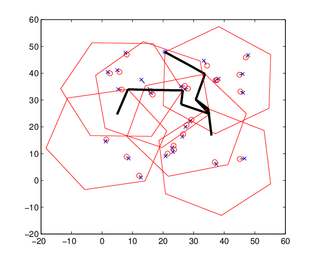
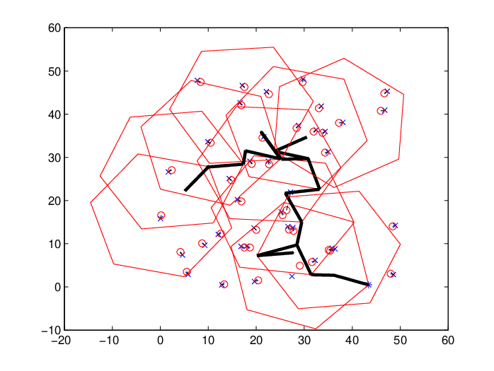
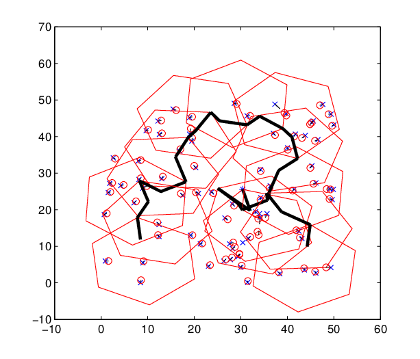
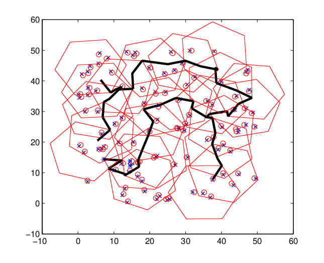
We have used MATLAB platform to study the performances of our proposed schemes. We have randomly generated a connected graph of sensors in a 50 meter $\times$ 50 meter square region. According to the section 3, we have taken values of beacon distance $u<r/7.5$. Following Figure 7 and Figure 8 show the hexagonal movement path (red solid lines) of a mobile anchor through the network during localization, where black bold lines are transition path between LRHs. The blue crosses and red circles are the actual and calculated positions of the sensors respectively and pairs are joined by dotted lines. The number of sensors $n$, communication ranges $r$, path length $D$ and average positioning error are given in the caption of each figure. All the values showing in the tables and figures are in meter. As the area remains fixed and connectivity is maintained by increasing communication range of sensors and the anchor, path length does not decrease much with the number of sensors.

In Table 2, we have shown localization error for different communication ranges $r$ and beacon distances $u$. According to Table 2, localization error decreases as beacon distance decreases for any fixed communication range. Here, $u=r/k$, where $k>7.5$ according to Theorem 5 and Theorem 6. We have also shown path lengths of the mobile anchor for different number of sensors forming a connected network in a square region of fixed side length 50 meter in Table 3. Here we keep the communication range fixed at 10 meter. Results show that path length does not increase much with number of sensors. It happens since degree of connectivity increases with the number of sensors in a fixed region.

Next we show the simulation results for the path planning scheme for a bounded square region. We have simulated the proposed scheme for a bounded region by varying $X$ from $r/10$ to $r/20$ and compared with [14]. We have fixed the value of communication range $r=10$ meter. We have compared path lengths with the existing schemes by varying $X$ for a fixed square region with side length $L=200$ meter. Results are shown in Table 4.

We have shown the percentages of improvement of our scheme over various schemes compared to path length for $r=10$ in Table 5. We have taken averages for different $X$ values to find average improvement on path length. Results show $13.45\%$ to $25.35\%$ improvement over different schemes. We have also shown values of average localization error of our scheme in Table 6 varying communication ranges $r$ and beacon distance $u$. We have taken $X=u$ in Table 6. Here also, localization error decreases as beacon distance decreases for any fixed communication range.

In this paper we have proposed path planning for a mobile anchor in a connected network and also in a bounded rectangular region. Our movement strategy reduces the requirement of three beacon points for localization to two beacon points, which helps improving path length for a rectangular region. In a connected network, once a sensor is localized, our path planning is able to localize all its neighbors with one hexagonal movement around the sensor. After completing one hexagonal movement, anchor decides its next destination depending upon received information from the neighboring sensors and localize all sensors along the way it moves. The novelty is that without knowing the boundary of the network, our distributed algorithm localizes all sensors using connectivity without any range estimation. We have also computed the length of the path traversed by the anchor for different number of sensors with good localization accuracy based on simulation. We have compared path length of our proposed movement strategy for rectangular region theoretically with existing literature to show better performance. Simulation results show $13.45\%$ to $25.35\%$ improvement of our path planning strategy over existing strategies in terms of path length of mobile anchor for rectangular region. In future we will try to investigate path planning in presence of obstacles.

The first author is thankful to the Council of Scientific and Industrial Research (CSIR), Govt. of India, for financial support during this work.

References

- [1] Galstyan A., Krishnamachari B., Lerman K., and Pattem S. Distributed online localization in sensor networks using a moving target. In Third International Symposium on Information Processing in Sensor Networks, 2004. IPSN 2004, pages 61–70, 2004.
- [2] Waleed Ammar, Ahmed ElDawy, and Moustafa Youssef. Secure localization in wireless sensor networks: A survey. CoRR, abs/1004.3164, 2010.
- [3] C. T. Chang, C. Y. Chang, and C. Y. Lin. Anchor-guiding mechanism for beacon-assisted localization in wireless sensor networks. IEEE SENSORS JOURNAL, 12(5):1098–1111, 2012.
- [4] Hongyang Chen, Gang Wang, Zizhuo Wang, Hing-Cheung So, and H Vincent Poor. Non-line-of-sight node localization based on semi definite programming in wireless sensor networks. IEEE Transaction on Wireless Communication, 11(1):108–116, 2012.
- [5] Sylvie Delaët, Partha Sarathi Mandal, Mariusz A. Rokicki, and Sébastien Tixeuil. Deterministic secure positioning in wireless sensor networks. Theoretical Computer Science, 412(35):4471 – 4481, 2011.
- [6] Han G., Xu H., Jiang J., Shu L., Hara T., and Nishio S. Path planning using a mobile anchor node based on trilateration in wireless sensor networks. Wireless Communications and Mobile Computing, 13(14):1324–1336, 2013.
- [7] Rui Huang and Gergely V. Záruba. Static path planning for mobile beacons to localize sensor networks. In PerCom Workshops, pages 323–330, 2007.
- [8] Kyunghwi Kim, Byunghyuk Jung, Wonjun Lee, and Ding-Zhu Du. Adaptive path planning for randomly deployed wireless sensor networks. J. Inf. Sci. Eng., 27(3):1091–1106, 2011.
- [9] Dimitrios Koutsonikolas, Saumitra M. Das, and Y. Charlie Hu. Path planning of mobile landmarks for localization in wireless sensor networks. Computer Communications, 30(13):2577–2592, 2007.
- [10] Sangho Lee, Eunchan Kim, Chungsan Kim, and Kiseon Kim. Localization with a mobile beacon based on geometric constraints in wireless sensor networks. IEEE Transactions on Wireless Communications, 8(12):5801–5805, 2009.
- [11] Hongjun Li, Jianwen Wang, Xun Li, and Hongxu Ma. Real-time path planning of mobile anchor node in localization for wireless sensor networks. In International Conference on Information and Automation, 2008. ICIA 2008., pages 384 – 389, 2008.
- [12] Xu Li, Nathalie Mitton, Isabelle Simplot-Ryl, and David Simplot-Ryl. Dynamic beacon mobility scheduling for sensor localization. IEEE Trans. Parallel Distrib. Syst., 23(8):1439–1452, 2012.
- [13] Sichitiu M.L. and Ramadurai V. Localization of wireless sensor networks with a mobile beacon. In IEEE International Conference on Mobile Ad-hoc and Sensor Systems, 2004, pages 174–183, 2004.
- [14] Chia-Ho Ou. Path planning algorithm for mobile anchor-based localization in wireless sensor networks. IEEE SENSORS JOURNAL, 13(2):466–475, 2013.
- [15] Chee Kiat Seow and Soon Yim Tan. Non-line-of-sight localization in multipath environments. IEEE Transactions on Mobile Computing, 7:647–660, May 2008.
- [16] Chia-Yen Shih and Pedro José Marrón. COLA: Complexity-reduced trilateration approach for 3D localization in wireless sensor networks. SENSORCOMM ’10, pages 24–32, Washington, DC, USA, 2010. IEEE Computer Society.
- [17] Kuo-Feng Ssu, Chia-Ho Ou, and Hewijin Christine Jiau. Localization with mobile anchor points in wireless sensor networks. IEEE T. Vehicular Technology, 54(3):1187–1197, 2005.
- [18] Bin Xiao, Hekang Chen, and Shuigeng Zhou. Distributed localization using a moving beacon in wireless sensor networks. IEEE Trans. Parallel Distrib. Syst., 19(5):587–600, 2008.
- [19] Yanchao Zhang, Wei Liu, Yuguang Fang, and Dapeng Wu. Secure localization and authentication in ultra-wideband sensor networks. IEEE Journal on Selected Areas in Communications, 24(4):829–835, 2006.