Hubble Frontier Fields First Complete Cluster Data: Faint Galaxies at
for UV Luminosity Functions and Cosmic Reionization
Note: Accepted for publication in The Astrophysical Journal
Abstract
We present the comprehensive analyses of faint dropout galaxies up to with the first full-depth data set of Abell 2744 lensing cluster and parallel fields observed by the Hubble Frontier Fields (HFF) program. We identify dropouts at in the HFF fields, and enlarge the size of galaxy sample obtained to date. Although the number of highly magnified () galaxies is small due to the tiny survey volume of strong lensing, our study reaches the galaxies’ intrinsic luminosities comparable to the deepest-field HUDF studies. We derive UV luminosity functions with these faint dropouts, carefully evaluating the combination of observational incompleteness and lensing effects in the image plane by intensive simulations including magnification, distortion, and multiplication of images, with the evaluations of mass model dependences. Our results confirm that the faint-end slope, , is as steep as at , and strengthen the evidence of the rapid decrease of UV luminosity densities, , at from the large sample. We examine whether the rapid decrease trend can reconcile with the large Thomson scattering optical depth, , measured by CMB experiments allowing a large space of free parameters such as average ionizing photon escape fraction and stellar-population dependent conversion factor. No parameter set can reproduce both the rapid decrease and the large . It is possible that the decrease moderates at , that the free parameters significantly evolve towards high-, or that there exist additional sources of reionization such as X-ray binaries and faint AGNs.
Subject headings
dark ages, reionization, first stars – galaxies: formation – galaxies: evolution – galaxies: high-redshift – gravitational lensing: strongI. Introduction
Cosmic reionization history and sources of reionization are open questions in astronomy today. Studies of QSO Gunn-Peterson absorption indicate that the intergalactic medium (IGM) is rapidly ionized at (Fan et al. 2006). A moderately large neutral hydrogen fraction at is implied by the Ly damping wing absorption features in the spectra of gamma-ray bursts (GRBs) at (Totani et al. 2006; Totani et al. 2013) and Ly emitters at (Kashikawa et al. 2006; Ouchi et al. 2010; Kashikawa et al. 2011; Konno et al. 2014). Similarly, there are reports of Ly-emitting galaxy fraction drops at probably due to the increase of Ly damping wing absorption given by the neutral hydrogen in the IGM (Pentericci et al. 2011; Pentericci et al. 2014; Ono et al. 2012; Schenker et al. 2012; Schenker et al. 2014; Treu et al. 2013; Finkelstein et al. 2013). Recent observations of cosmic microwave background (CMB) present the large value of the Thomson scattering optical depth (Planck Collaboration et al. 2013). The large value of indicates that the reionization takes place at if an instantaneous reionization is assumed. The combination of these data implies that the reionization process is extended at .
Star-forming galaxies are thought to be major sources of the cosmic reionization (see reviews of Fan et al. 2006; Robertson et al. 2010). Recent ultra-deep observations with the Wide Field Camera 3 (WFC3) aboard the Hubble Space Telescope (HST) have provided improved estimates of the abundances of star-forming galaxies at (Ellis et al. 2013; Schenker et al. 2013; McLure et al. 2013). Combining these results with the WMAP constraints on the Thomson scattering optical depth (Hinshaw et al. 2013) and stellar mass densities, Robertson et al. (2013) suggest that all these observations can be explained consistently if their population of star-forming galaxies extends below the survey limits down to absolute UV magnitudes of . However, it is difficult to translate the UV luminosity function measurements into the ionized hydrogen fraction, because of uncertainties of the following three unknown parameters. The first is the escape fraction , which is the fraction of the numbers of ionizing photons escaping into the IGM to those produced by star-formation in a galaxy. The second is the conversion factor , which converts a UV luminosity density to the ionizing photon emission rate in a star-forming galaxy. The third is a clumping factor , where are the local number density of ionized hydrogen and the brackets indicate spatial average. It is critically important to take into account the uncertainties of these parameters to estimate the contribution of galaxies to reionization.
Moreover, the abundance of faint galaxies at high redshift is unknown. Some theoretical studies indicate that the star formation is suppressed in low-mass halos. Boylan-Kolchin et al. (2014) suggest that the star formation is suppressed in halos smaller than at high redshift, corresponding to . Cosmological hydrodynamical simulations of Jaacks et al. (2013) exhibit a turnover of the UV luminosity function at . Thus it is not obvious if the UV luminosity function of star-forming galaxies indeed extends down to , as assumed in Robertson et al. (2013). Recent observations of nearby dwarf galaxies find that the star formation in dwarf galaxies is suppressed at the epoch of reionization (Benitez-Llambay et al. 2014; Weisz et al. 2014). The faint-end slope of the UV luminosity function is also not well known at high redshift. The steepening of UV luminosity functions towards high- is a general agreement of observational studies. Bouwens et al. (2014) conclude that the value of evolves from at to at . However, the determination of includes a large uncertainty at , due to the poor statistics of the luminosity function measurement.
Gravitational lensing by massive clusters is an effective tool to reveal properties of faint galaxies at high redshift. Lensing magnifications of background sources enable us to observe intrinsically faint sources that are not detected without lensing magnifications. For example, Cluster Lensing And Supernova survey with Hubble (CLASH) studies properties of faint star-forming galaxies at using the lensing technique (Bouwens et al. 2012; Bradley et al. 2013). Recently, HST has started revolutionary deep imaging on the six massive clusters with parallel observations, the Hubble Frontier Fields (HFF; PI: J. Lotz) project whose data are mag deeper than those of CLASH. The HFF project identifies faint sources reaching 29 AB mag, allowing us to detect background sources with intrinsic magnitudes of mag by lensing magnification (Coe et al. 2014). The HFF first targets the Abell 2744 cluster, followed by other five clusters: MACSJ0416.1-2403, MACSJ0717.5+3745, MACSJ1149.5+2223, Abell S1063 (RXCJ2248.7-4431), and Abell 370. The observations of Abell 2744 were just completed in July 2014, which provide the first full-depth data set on an HFF target.
In this paper, we identify star-forming galaxies at magnified by gravitational lensing in the Abell 2744 cluster and its parallel fields. We refer to the former as the cluster field and the latter as the parallel field in the remainder of this paper. This work serves as a precursor study that uses the first one sixth of the full-depth HFF data set. We construct the mass model of Abell 2744, and derive the UV luminosity functions with the star-forming galaxies at . Calculating the UV luminosity densities from the UV luminosity functions of our and previous studies, we discuss cosmic reionization based on the UV luminosity density measurements and Thomson scattering optical depths from CMB observations with the ionization equation that allows a large free parameter space.
We present details of the observational data in Section II. The photometric catalog and dropout selection methods are described in Section III, and our mass model of Abell 2744 is presented in Section IV. Using these data, we derive the parameters of UV luminosity functions in Section V. In Section VI, we discuss cosmic reionization with the UV luminosity densities and Thomson scattering optical depths. Finally, we summarize our results in Section VII. We adopt a cosmology with , , , and km s-1 Mpc-1.
II. Data
The Abell 2744 cluster and the parallel fields were observed with WFC3-IR and Advanced Camera for Survey (ACS)
in the HFF project.
These data were reduced and released to the public through the HFF official website.
11
1
http://archive.stsci.edu/pub/hlsp/frontier/abell2744/
images/hst/v1.0/
They provide drizzled science images and inverse variance weight images
in four WFC3-IR bands, F105W (), F125W (), F140W (), and F160W (),
and
in three ACS bands, F435W (), F606W (), and F814W ().
We use version 1.0 of the public images with a pixel scale of pixel-1.
For the measurements of object colors,
we homogenize the point spread functions (PSFs) of the WFC3 images with iraf (Tody 1986; Tody 1993) imfilter package.
A summary of the HST data is shown in Table 1.
We measure limiting magnitudes in a -diameter circular
aperture using sdfred (Yagi et al. 2002; Ouchi et al. 2004).
We find that the limits are
mag in the cluster field and mag in the parallel field.
The cluster field contains the bright intracluster light (Montes & Trujillo 2014),
which makes the depths of the cluster field shallower than those of the parallel field.
The limiting magnitudes presented in Table 1 are measured in the entire field. However, the intracluster light is brighter in the cluster center than in the outskirts, which causes spatial variations of the depth in the HST images. To evaluate the spatial variations, we measure the limiting magnitudes in each of grid cells defined in Figure 1. We present the -band limiting magnitudes in the cells in Figure 1. In Figure 1, we find that the depth in the third-row second-column cell ( mag) is about mag shallower than those of the cluster outskirts ( mag) due to the bright intracluster light. The peak-to-peak magnitudes of spatial variations of the depths are also mag in the rest of WFC3-IR images and the ACS data. In the cluster field, we adopt the space-dependent limiting magnitudes as illustrated in Figure 1. For sources in the outside of the cell, we apply a limiting magnitude of the nearest cell.
| Filter | Orbits | Detection LimitsaaMeasured in a -diameter circular aperture. | PSF FWHM |
|---|---|---|---|
| arcsec | |||
| Cluster Field | |||
| ()bbThe values in the parenthesis correspond to the detection limits and the PSF FWHMs of PSF-homogenized images. | ()bbThe values in the parenthesis correspond to the detection limits and the PSF FWHMs of PSF-homogenized images. | ||
| ()bbThe values in the parenthesis correspond to the detection limits and the PSF FWHMs of PSF-homogenized images. | ()bbThe values in the parenthesis correspond to the detection limits and the PSF FWHMs of PSF-homogenized images. | ||
| ()bbThe values in the parenthesis correspond to the detection limits and the PSF FWHMs of PSF-homogenized images. | ()bbThe values in the parenthesis correspond to the detection limits and the PSF FWHMs of PSF-homogenized images. | ||
| ()bbThe values in the parenthesis correspond to the detection limits and the PSF FWHMs of PSF-homogenized images. | ()bbThe values in the parenthesis correspond to the detection limits and the PSF FWHMs of PSF-homogenized images. | ||
| ()bbThe values in the parenthesis correspond to the detection limits and the PSF FWHMs of PSF-homogenized images. | ()bbThe values in the parenthesis correspond to the detection limits and the PSF FWHMs of PSF-homogenized images. | ||
| ccThe detection image for - and -dropout selections. | |||
| ddThe detection image for -dropout selection. | |||
| Parallel Field | |||
| ()bbThe values in the parenthesis correspond to the detection limits and the PSF FWHMs of PSF-homogenized images. | ()bbThe values in the parenthesis correspond to the detection limits and the PSF FWHMs of PSF-homogenized images. | ||
| ()bbThe values in the parenthesis correspond to the detection limits and the PSF FWHMs of PSF-homogenized images. | ()bbThe values in the parenthesis correspond to the detection limits and the PSF FWHMs of PSF-homogenized images. | ||
| ()bbThe values in the parenthesis correspond to the detection limits and the PSF FWHMs of PSF-homogenized images. | ()bbThe values in the parenthesis correspond to the detection limits and the PSF FWHMs of PSF-homogenized images. | ||
| ()bbThe values in the parenthesis correspond to the detection limits and the PSF FWHMs of PSF-homogenized images. | ()bbThe values in the parenthesis correspond to the detection limits and the PSF FWHMs of PSF-homogenized images. | ||
| ()bbThe values in the parenthesis correspond to the detection limits and the PSF FWHMs of PSF-homogenized images. | ()bbThe values in the parenthesis correspond to the detection limits and the PSF FWHMs of PSF-homogenized images. | ||
| ccThe detection image for - and -dropout selections. | |||
| ddThe detection image for -dropout selection. | |||

III. Samples
In this section, we select the -, -, and dropout candidates in the cluster and the parallel fields with the color criteria from our source catalogs. We also compare our dropout samples with those obtained in previous studies.
III.1. Photometric catalog
Using SWarp (Bertin et al. 2002), we make two detection images that are co-added data of and for our - and -dropout candidates and -dropout candidates, respectively. We match the PSFs of these band images in the same manner as the WFC3-IR images (Section II), and produce the detection images. To apply the criteria of no blue-continuum detections for our dropout selections, we do not match the PSFs of the blue bands whose wavelengths are shorter than the redshifted Ly-break feature of our dropout candidates. Because the PSF-unmatched images in the blue bands provide upper limits on the flux densities that are stronger than PSF-homogenized images for point-like sources of high- galaxies, we use the PSF-unmatched data of the individual ACS images to obtain the upper limits.
We construct our source catalogs from the HFF images using SExtractor (Bertin & Arnouts 1996) in a total of arcmin2 area where all the WFC3 and ACS images are available. We run SExtractor in dual-image mode for each set of the images. In the cluster field, we set DEBLEND_NTHRESH to and DEBLEND_MINCONT to a small value of in order to detect objects even in highly crowded regions. In the parallel field, we use more conservative values, and , because the parallel field are not crowded. 22 2 Although we use the different deblending parameter sets in the cluster and the parallel fields, this difference does not affect our final results of the UV luminosity functions. This is because we use the same deblending parameter sets, each for the cluster and parallel fields, self-consistently in our simulations to derive our UV luminosity functions (Section V). The number of objects identified in the detection images is in total. The colors of the objects are measured with magnitudes of MAG_APER (), which are estimated from the flux density within a fixed circular aperture. The aperture diameters used for are two times of the FWHMs of the PSFs. We adopt the diameters of () and for the PSF-matched images and for the PSF-unmatched blue-band images in the cluster (parallel) field, respectively. The detection limits are also defined with () diameter apertures for the PSF-matched images, and diameter apertures for the PSF-unmatched images in the cluster (parallel) field.
We apply an aperture correction that is defined by the following procedure. We create a median stacked -band image of our dropout candidates selected in Section III.2, and measure the aperture flux of the stacked dropout candidate as a function of aperture size. Because the flux almost levels off at around a diameter, we regard the flux within a -diameter aperture as the total flux corresponding to the total magnitude . In the stacked image, is fainter than by mag. We thus estimate the total magnitudes with , where is the aperture correction factor of mag. We also make median stacked images for bright and faint subsamples of our dropout candidates, and obtain values. We confirm that the values of do not depend on luminosity beyond the statistical uncertainties in the magnitude range of our dropout candidates. Thus we apply one aperture correction factor of for all our dropout candidates.
To check the accuracy of our aperture correction, we compare with the magnitude of MAG_AUTO (), which is calculated with the Kron elliptical aperture (Kron 1980). Figure 2 presents as a function of , and indicates that is comparable to for bright dropout candidates with mag. The values of have significant scatters at the faint magnitudes, which is mainly due to uncertainties in determining the Kron elliptical apertures of faint sources. We adopt for our estimates of total magnitudes, as we expect that the values are more reliable than for faint sources.
III.2. Dropout Selection
For the selection of -dropouts at , we use the color criteria defined by Atek et al. (2014b):
| (1) | |||
| (2) | |||
| (3) |
For objects fainter than the limiting magnitude in , upper limiting magnitude is replaced with the magnitude (see Atek et al. 2014b). For secure source detection, we apply the source identification thresholds of the significance levels both in the and bands. From our -dropout candidate catalog, we remove sources detected at the level either in the or band.
For -dropouts at , we adopt the following criteria (Schenker et al. 2013):
| (4) | |||
| (5) |
As described in Schenker et al. (2013), we use the upper limiting magnitude in the band. In this selection, sources with the levels both in the and bands are regarded as real objects. We reject sources detected at in the optical bands. Additionally, we apply a criterion that no more than one of the optical bands shows a detection above the level. We use a collective value to eliminate contamination, the details of which are described in Section 3.3 of Bouwens et al. (2011) and Section 3.2 of Schenker et al. (2013). The corrective is defined by , where is the flux density in the -th band, is the signal-to-noise ratio of the source in the -th band, and is a sign function; if and if . The index runs across , , and . We remove objects with from our dropout candidates if they are brighter than the limit in the band, and remove ones with if they are fainter than the limit. A linear interpolation is used for objects with between the and limit.
For -dropouts at , we use the following criteria:
| (6) | |||
| (7) | |||
| (8) | |||
| (9) |
We replace the or magnitude with the upper limiting magnitude if an object is fainter than the magnitude in or , following Oesch et al. (2013). For the -dropouts, we require detection significance levels beyond in the and bands, and in at least one of the and bands. From our -dropout sample, we remove sources detected at the level in, at least, one of the optical bands and sources with . These criteria are similar to those defined by Oesch et al. (2013), but we slightly relax the criteria to include dropout candidates at .
We select -, -, and -dropouts with the selection criteria shown above. Figure 3 shows the two-color diagrams for our dropout candidates, together with the expected tracks of high-redshift star-forming galaxies with UV slopes of and (see Meurer et al. 1999 for the definition of ). Our dropout samples consist of -dropout, -dropout, and -dropout candidates. These dropout candidates are listed in Tables 2-4. Figure 4 shows cutout images of our dropout candidates. Note that two out of -dropout candidates are the objects which are also selected as -dropout candidates. The numbers of dropout candidates in the cluster field are comparable to those in the parallel field, although the cluster field is subject to the strong lensing effects. The numbers of dropout candidates are affected by two effects of the lensing magnification. One is the magnification of surface brightness that enhances the observed brightness of the dropout candidates. The other is the magnification of the observed area, which reduces the effective survey area on the source plane. In the numbers of dropout candidates, these two effects compensate (Coe et al. 2014). Albeit the small statistics of a single HFF pointing, this would be one of the reasons why the numbers of dropout candidates are similar in the cluster and the parallel fields. More quantitative arguments of the lensing effects are presented in Section V.
We estimate photometric redshifts of our dropout candidates using the Bayesian photometric redshift code bpz (Benítez 2000). Tables 2, 3, and 4 include the photometric redshifts. The redshift ranges are -, -, and for the -, , and -dropout candidates, except a candidate with the ID of HFF1P-i12 at . The three samples of dropout candidates cover . We confirm that the ranges of the photometric redshifts are consistent with the redshifts defined by the dropout selections, , , and . In the remainder of this paper, we refer to -, -, and -dropout candidates as , , dropouts, respectively.

Recently, Atek et al. (2014b), Zheng et al. (2014), Coe et al. (2014), and Atek et al. (2014a) have identified a total of 16, 18, 7, and 58 dropouts at in the Abell 2744 cluster field, respectively. We recover , , , and dropouts of their samples. Laporte et al. (2014) analyze the spectral energy distribution of a dropout, which is identified in our selection with the ID of HFF1C-Y1 and in all the other three studies. Our dropout with the ID of HFF1C-Y9 is also found in Zheng et al. (2014) as one of the three multiple images. Although we find HFF1C-Y9 by the -dropout selection, Zheng et al. (2014) identify the multiply-imaged object as an -dropout. The different selections of - and -dropouts are explained by the fact that the photometric redshift of HFF1C-Y9 is that is the border value of the -dropout and -dropout redshift ranges. Zitrin et al. (2014) have reported a triply-imaged dropout in the cluster field (see also Oesch et al. 2014). We recover one of the multiple images as a -dropout with the ID of HFF1C-YJ1. In Section IV.4, we discuss the multiple images including HFF1C-Y9 and HFF1C-YJ1 with our mass model.
We do not recover , , , and dropouts found in Atek et al. (2014b), Zheng et al. (2014), Coe et al. (2014), and Atek et al. (2014a), respectively. The difference of our and their samples can be explained by the following three reasons. First, we use the full-depth images of HFF Abell 2744 observations, while Atek et al. (2014b), Zheng et al. (2014), and Coe et al. (2014) only use relatively shallow ACS images observed in HST Cycle 17 (GO 11689, PI: Dupke). Second, the limiting magnitude definitions are different. We take account of the space-dependent limiting magnitudes in the cluster field as described in Section II. Third, there are differences in galaxy selection techniques. Zheng et al. (2014) and Coe et al. (2014) do not use the well-tested color selections, but sophisticated photometric redshifts for the selections. Although we concur with all 9 confident dropouts from Zheng et al. (2014), we recover only one dropout from Zheng et al. (2014). Similarly, we recover only 19 out of 50 dropouts at from Atek et al. (2014a). This is possibly because our selection criteria for our dropouts are more conservative than those of Zheng et al. (2014) and Atek et al. (2014a).
| ID | R.A. (J2000) | Dec (J2000) | aaTotal magnitudes estimated with the aperture correction. | MagnificationbbThe magnification errors in the parallel field are less than based on our model extrapolation estimates. Note that the errors in the parallel field would be underestimated because Abell 2744 is a complex merging cluster. | Photo- | ReferenceccReferences: (1) Atek et al. (2014b); (2) Zheng et al. (2014); (3) Atek et al. (2014a) | ||
|---|---|---|---|---|---|---|---|---|
| Cluster field | ||||||||
| HFF1C-i1 | , | |||||||
| HFF1C-i2 | , | |||||||
| HFF1C-i3 | , | |||||||
| HFF1C-i4 | , | |||||||
| HFF1C-i5 | , | |||||||
| HFF1C-i6 | , | |||||||
| HFF1C-i7 | ||||||||
| HFF1C-i8 | , | |||||||
| HFF1C-i9 | , | |||||||
| HFF1C-i10 | ||||||||
| HFF1C-i11 | ||||||||
| HFF1C-i12 | , , | |||||||
| HFF1C-i13 | ||||||||
| HFF1C-i14 | ||||||||
| HFF1C-i15 | ||||||||
| HFF1C-i16 | ||||||||
| HFF1C-i17 | ||||||||
| HFF1C-i18 | ||||||||
| Parallel field | ||||||||
| HFF1P-i1 | ||||||||
| HFF1P-i2 | ||||||||
| HFF1P-i3 | ||||||||
| HFF1P-i4 | ||||||||
| HFF1P-i5 | ||||||||
| HFF1P-i6 | ||||||||
| HFF1P-i7 | ||||||||
| HFF1P-i8 | ||||||||
| HFF1P-i9 | ||||||||
| HFF1P-i10 | ||||||||
| HFF1P-i11 | ||||||||
| HFF1P-i12 | ||||||||
| HFF1P-i13 | ||||||||
| HFF1P-i14 | ||||||||
| HFF1P-i15 | ||||||||
| HFF1P-i16 | ||||||||
| HFF1P-i17 | ||||||||
.
| ID | R.A. (J2000) | Dec (J2000) | aaTotal magnitudes estimated with the aperture correction. | MagnificationbbThe magnification errors in the parallel field are less than | Photo- | ReferenceccReferences: (1) Atek et al. (2014b); (2) Zheng et al. (2014); (3) Zheng et al. (2014) possible candidates; (4) Coe et al. (2014); (5) Laporte et al. (2014); (6) Atek et al. (2014a). | ||
|---|---|---|---|---|---|---|---|---|
| Cluster field | ||||||||
| HFF1C-Y1 | , , , , | |||||||
| HFF1C-Y2 | , , | |||||||
| HFF1C-Y3 | , , | |||||||
| HFF1C-Y4 | , , | |||||||
| HFF1C-Y5 | , , | |||||||
| HFF1C-Y6 | , | |||||||
| HFF1C-Y7 | , , | |||||||
| HFF1C-Y8 | , | |||||||
| HFF1C-Y9 | , | |||||||
| HFF1C-Y10 | ||||||||
| HFF1C-Y11 | ||||||||
| Parallel field | ||||||||
| HFF1P-Y1 | ||||||||
| HFF1P-Y2 | ||||||||
| HFF1P-Y3 | ||||||||
| HFF1P-Y4 | ||||||||
.
| ID | R.A. (J2000) | Dec (J2000) | aaTotal magnitudes estimated with the aperture correction. | MagnificationbbThe magnification errors in the parallel field are less than | Photo- | ReferenceccReferences: (1) Zitrin et al. (2014); (2) Oesch et al. (2014); (3) Zheng et al. (2014); (4) Coe et al. (2014); (5) Atek et al. (2014a). | ||
|---|---|---|---|---|---|---|---|---|
| Cluster field | ||||||||
| HFF1C-YJ1 | , | |||||||
| HFF1C-Y2ddIdentified by our two selections for -dropouts and -dropouts. | ,, | |||||||
| HFF1C-Y5ddIdentified by our two selections for -dropouts and -dropouts. | ,, | |||||||
| Parallel field | ||||||||
| HFF1P-YJ1 | ||||||||
| HFF1P-YJ2 | ||||||||
| HFF1P-YJ3 | ||||||||
.
IV. Mass Model
In this section, we construct a mass model of Abell 2744 at using the parametric gravitational lensing package glafic (Oguri 2010). 33 3 we name the mass model in this work ’glafic model version 1.0’. This mass model will be released on the STScI website (http://archive.stsci.edu/prepds/frontier/lensmodels/). The mass model version 2.0 is being developed, in which we include new multiple images. Our mass model includes three types of mass distributions: cluster-scale halos, cluster member galaxy halos, and external perturbation. With the positions of multiple images provided in the literature, we optimize free parameters of the mass profiles based on a standard minimization to determine the best-fit mass model whose parameters are summarized in Table 5. We then calculate magnification factors of our dropouts and positions of the multiple images using the best-fit mass model.
IV.1. Cluster-Scale Halos
We place three cluster-scale halos at the positions of three brightest galaxies in the core of the cluster. We adopt the Navarro-Frenk-White (NFW) profiles (Navarro et al. 1997) for the mass distributions of the cluster-scale halos. The radial profiles of NFW are described as
| (10) |
where is the characteristic density and is the scale radius. The scale radius is defined by
| (11) |
where is the virial radius of the cluster-scale halo and is the concentration parameter. The scale radius and the characteristic density are related to the virial mass and the concentration parameter with the equations,
| (12) | ||||
| (13) | ||||
| (14) |
where is the nonlinear overdensity (Nakamura & Suto 1997, e.g.,) and is the mean matter density of the universe at a redshift . The surface mass density is obtained as a function of a radius by integrating along the line of sight:
| (15) |
In the obove discussion, we assumed spherical halos. We then introduce an ellipticity in the isodensity contour by replacing in (Oguri 2010):
| (16) |
where and are defined by the following equations with the position angle (measured east of north) of the isodensity contours:
| (17) | |||
| (18) |
We use the ellipsoidal halos in this work. Each cluster-scale halo has four free parameters: , , , and .
| Component | model | Mass () | (∘) | R.A. (J2000) | Dec (J2000) | ||
|---|---|---|---|---|---|---|---|
| Cluster halo 1 | NFW | ||||||
| Cluster halo 2 | NFW | ||||||
| Cluster halo 3 | NFW | ||||||
| (km s-1) | (′′) | ||||||
| Member galaxies | PJE | ||||||
| (∘) | |||||||
| Perturbation | PRT | (fix) | (fix) |
IV.2. Cluster Member Galaxy Halos
To estimate contributions from cluster member galaxy halos, we identify cluster member galaxies with spectroscopic redshifts , photometric redshifts , and colors. First, we use presented in Table 5 of Owers et al. (2011). Galaxies at are regarded as cluster member galaxies. For objects with no , we apply color criteria,
| (19) | ||||
| (20) | ||||
| (21) |
and select galaxies on the red-sequence of the cluster redshift. Figure 5 presents the versus color-magnitude diagram of our objects, together with the color criteria of the red-sequence galaxies shown with the solid-line box. Finally, for objects that are selected neither by nor the red-sequence criteria, we refer estimated with bpz (Section III). We select member galaxies with the criterion and the relaxed color-magnitude criteria,
| (22) | ||||
| (23) | ||||
| (24) | ||||
| (25) |
The dashed-line box in Figure 5 indicates the boundary of the relaxed color-magnitude criteria.
We describe halo mass distributions of these member galaxies by the sum of pseudo-Jaffe ellipsoids (PJE; Keeton 2001, see also Jaffe 1983). In this model, the mass profile is characterized by the velocity dispersion and the truncation radius . We assume that the parameters of and are scaled with the galaxy luminosity in the band,
| (26) | ||||
| (27) |
where is the normalization luminosity at the cluster redshift, and , , and are free parameters. The mass-to-light ratio is constant for . The ellipticities and position angles of the member galaxy halos are determined from shapes of the member galaxies in the band.
IV.3. External Perturbation
Although the mass distribution of Abell 2744 is mostly explained by the contributions from the three cluster-scale halos (Section IV.1) and the member galaxy halos (Section IV.2), we include perturbation induced by external sources to improve our mass model. If the perturbation is weak, its potential can be described by (Kochanek 1991, e.g.,)
| (28) |
where is the constant convergence and is the constant tidal shear. The amplitude of the potential is defined for a given fiducial source redshift . We refer to this potential as PRT. In this paper, and are free parameters. We fix and ; and .
IV.4. Model Optimization
To constrain the mass-model parameters of the cluster, we use the positions of multiply imaged systems.
We identify multiply imaged galaxies based on their colors and morphologies
while iteratively refining the mass-model parameters.
In total, we use the positions of multiple images of systems summarized in Table 6.
Seventeen out of the systems, IDs (Table 6),
are the same as those listed in Table 1 of the document provided by the HFF map-making team (PI: K. Sharon; see also Johnson et al. 2014)
44
4
http://archive.stsci.edu/prepds/frontier/lensmodels/
hlsp_frontier_model_abell2744_sharon_v1_readme.pdf.
Similarly, four high-redshift systems from the systems, IDs , are
listed in Table 3 of Atek et al. (2014b),
among which IDs , , and are identified as dropouts in Section III.2.
The images of IDs , , and are referred to
as HFF1C-i5, HFF1C-i6, and HFF1C-i8 in Table 2.
We also find three new sets of multiple images, IDs and .
We search for the best-fit mass model which reproduces the positions of the multiple images. We optimize the 23 free parameters described in Section IV.1-IV.3 based on a minimization with the downhill-simplex algorithm (See Oguri 2010 for more details). We assign a positional error of in the image plane for each multiple image, following Oguri (2010), and obtain the best-fit parameters as summarized in Table 5. The best-fit model has for degrees of freedom, suggesting that our model is reasonable.
In the following sections, we use this best-fit mass model to estimate the lensing effects both in the cluster and parallel fields. Because the parallel field has no multiple images to constrain the parameters of the mass model, it should be noted that the lensing effects in the parallel field are estimated from the extrapolation of the mass model determined at the cluster field. However, the extrapolation gives negligibly small uncertainties in our final results, due to the very small magnification factors (see Section IV.5).
| ID | R.A. (J2000) | Dec (J2000) | aaRedshift from the best-fit mass model. | bbNumbers quoted from Johnson et al. (2014). | bbNumbers quoted from Johnson et al. (2014). | ReferenceccReferences: (1) http://archive.stsci.edu/prepds/frontier/lensmodels/hlsp_frontier_model_abell2744_sharon_v1_readme.pdf, see also Johnson et al. (2014); (2) Atek et al. (2014b). |
|---|---|---|---|---|---|---|
| ddFixed to . | ||||||
| ddFixed to . | ||||||
IV.5. Magnification Factors and Multiple Images
Figure 6 displays the critical lines for sources and the positions of our dropouts in the cluster field. Because most of the dropouts are located far from the critical lines, the magnification factors are generally small, , as presented in Tables 2-4. However, some of the dropouts are placed near the critical line and highly magnified. In particular, the magnification factors of three dropouts, HFF1C-i10, HFF1C-Y9, and HFF1C-YJ1, are estimated to be . The intrinsic absolute magnitudes of these three dropouts are , , and mag, respectively. Figure 7 shows the positions of our dropouts in the parallel field. The magnification factors in the parallel field are almost the same and near unity, typically . Thus, the lensing effects in the parallel field are negligibly small, and the parallel field may be regarded as a blank field. Although the magnification of the parallel field is very small, we adopt the lensing magnifications to our dropouts both in the cluster and the parallel fields in our analysis. We estimate the errors of the magnification factors with a Markov Chain Monte Carlo (MCMC) method. These errors are shown in Tables 2-4.
Our mass model predicts that three systems in our dropout samples have counter images. We discuss the positions and the redshifts of these multiple images using our mass model. Because the predicted positions of multiple images depend on the source redshifts, we estimate the redshifts of multiple images from the positions in the image plane.
HFF1C-YJ1 at
HFF1C-YJ1 is a highly magnified dropout at which is also reported in Zitrin et al. (2014). Zitrin et al. (2014) claim two counter images of this dropout, which we refer to as HFF1C-YJ1-2 and HFF1C-YJ1-3. In Figure 8, we show the predicted positions of the counter images of HFF1C-YJ1 whose redshifts are assumed to be . The positions of the counter images are consistent with our estimates, if the redshift of HFF1C-YJ1 is . In fact, the predicted positions of the counter images are largely separated, , if HFF1C-YJ1 resides at . Thus our mass model predicts that the redshift of HFF1C-YJ1 is , which is consistent with the findings of Zitrin et al. (2014). The multiple image positions rule out the possibility that HFF1C-YJ1 is a low redshift galaxy at , and imply that the HFF1C-YJ1 system is a strong candidate of a high redshift galaxy. Combining the result of photometric redshift, we find that the system of HFF1C-YJ1, HFF1C-YJ1-2 and HFF1C-YJ1-3 is located at .
HFF1C-Y9 at
HFF1C-Y9 is a highly magnified dropout at . Zheng et al. (2014) find two counter images of this dropout, which are referred to as HFF1C-Y9-2 and HFF1C-Y9-3 in this paper. Figure 9 presents the predicted positions of the counter images of HFF1C-Y9. Our mass model predicts that HFF1C-Y9 has more than two counter images, if HFF1C-Y9 resides at . However, we cannot investigate the positions of these additional counter images due to the bright galaxies along the lines of sight. We compare the observed images of HFF1C-Y9-2 and HFF1C-Y9-3 with the predicted positions. The observed images fall in the predicted positions for the system at , implying that HFF1C-Y9 would be a source at a redshift slightly lower than that estimated in the dropout selection.
HFF1C-i5, -i6, and -i8 at
We find three multiple images of an -dropout, which are HFF1C-i5, HFF1C-i6, and HFF1C-i8. We use the positions of these three multiple images for the construction of our mass model. Their IDs in Table 6 are 19.1, 19.2, and 19.3, respectively. In addition to these three multiple images, Atek et al. (2014b) report another counter images, which is named Image 5.4 in Table 3 of Atek et al. (2014b). In our paper, we refer to Image 5.4 as HFF1C-i5-2. In Figure 10, we plot the predicted positions of these four multiple images. The predicted position of HFF1C-i5-2 is about away from the images reported by Atek et al. (2014b). Instead, it is close to the position predicted by Jauzac et al. (2014) shown with the green circle in Figure 10. The observed images of the other three multiple images lie near the predicted positions at and . Our mass model predicts that the best-fit value of their redshift is , as shown in Table 6.


IV.6. Comparisons with the Public Mass Models
Mass models of Abell 2744 are also made by other groups (e.g., Lam et al. 2014). Eight public mass models are accessible through the STScI website55 5 http://archive.stsci.edu/prepds/frontier/lensmodels/ which are made by the five independent groups, M. Bradač (PI), The Clusters As TelescopeS (CATS) team (Co-PI’s J.P Kneib, P. Natarajan; see Richard et al. 2014), J. Merten & A. Zitrin (Co-PI’s), K. Sharon (PI; see Johnson et al. 2014), and L. Williams (PI). Figure 11 compares the magnification factors of our mass model and these public mass models at the positions of our dropout candidates in the cluster field. The vertical axes show , where is the magnification factor from our mass model and is the difference between magnification factors of our model and a public mass model (). In the cluster field, the magnification factors from our mass model are broadly consistent with those from the public mass models. We especially find excellent agreements with the CATS and Zitrin-NFW models. The Merten’s group extends their mass model to the parallel field using weak lensing data covering both the cluster and parallel field. The magnification factors in the parallel field from the Merten model are . Our mass model estimates the magnifications of the dropouts in the parallel field to be , which is consistent with those from Merten model.
V. UV Luminosity Functions
In this section, we derive UV luminosity functions of dropout galaxies at , , and based on the dropouts identified by our HFF study and the previous blank field surveys. In Section V.1, we estimate the contamination rates of our dropout samples. In Section V.2, we conduct Monte Carlo simulations with the gravitational lensing effects, and in Section V.3 we obtain simulated number counts of dropouts in the image plane. Incorporating the contamination estimates, we search for the best-fit Schechter parameters for the UV luminosity functions of dropout galaxies at , , and .
V.1. Contamination Estimates
One of the major sources of contamination in high-redshift dropout galaxy samples is galaxies at whose Balmer break mimics a Lyman- break in the spectra of high- star-forming galaxies. Although bright interlopers are removed by detections of a blue continuum in deep optical images, faint interlopers are selected due to the photometric uncertainties. Here we estimate the expected number of such contaminants that meet our dropout selection criteria, basically following the method described in Section 3.3 of Schenker et al. (2013, see also Section 3.1 of ).
To obtain the expected number of contaminants,
we make use of our catalog
of bright objects
detected in the HFF fields.
We assume that
bright objects with that do not satisfy
the dropout selection criteria are bright interlopers,
and that faint interlopers have the color distribution same as that of bright ones.
We create artificial objects with faint magnitudes of
using the mkobjects package in iraf (Tody 1986; Tody 1993) software.
Their number counts are matched to
the observed number counts extrapolated from the bright magnitudes.
These artificial objects are placed in random positions of our HFF images.
We conduct the source extraction and the dropout selection in the same manner
as our dropout galaxy identification in the real HFF data.
The artificial objects selected as dropouts are regarded as contaminants.
We derive the numbers of contamination objects as a function of magnitude,
which is used in our UV luminosity function estimates in Section V.3.
We find that the fraction of total numbers of the contaminants to our dropout candidates
down to 29.5 magnitude is %.
This fraction is relatively larger than the contamination rate estimated by some previous studies, which are for examples at in Bouwens et al. (2011) and at in Bouwens et al. (2012).
In Section VI, we discuss the discrepancy between the UV luminosity densities and Thomson scattering optical depth.
Because the differences of the number counts given by the contamination estimates are at most 30% which is smaller than the discrepancy discussed in Section VI, our conclusion does not change.
V.2. Completeness Estimates
The gravitational lensing effects are important to interpret the observational results of our dropouts in the HFF fields. The brightness of dropouts are magnified, and multiple images appear for some of the dropouts. Thus, the number counts of our HFF dropout candidates are changed from those of the blank field by the gravitational lensing effects, especially in the cluster field. Moreover, to derive UV luminosity functions, one needs to correct for the selection incompleteness of dropouts that is a function of both magnitude and source redshift. In our study, we carry out Monte-Carlo simulations in the image plane to evaluate the gravitational lensing effects as well as the selection completeness. The simulations contain all lensing effects: magnification, distortion, and multiplication of images. This is called the image plane technique.
There is another method for the luminosity function estimates referred to as the source plane technique (Atek et al. 2014b). The source plane technique determines an absolute magnitude of each dropout candidate with a magnification factor to derive the number of dropout candidates per unit source plane volume. However, distortion and multiplication effects are not included in the source plane technique. Note that our method of the image plane technique is self-consistent and more complete than the source plane technique.
We first estimate the completeness of dropouts identified by our selections in the HFF images, where the completeness depends on redshift and magnitude. We create a mock catalog of galaxies uniformly distributed at in the magnitude range of mag. To define the UV continuum colors of the galaxies, we assume a spectral UV slope of , which is the same as that used in Schenker et al. (2013). IGM attenuation is given with the prescription given by Madau et al. (1996). For the galaxies’ intrinsic surface brightness profiles, we adopt a Sérsic index of and half-light radii of kpc and kpc for bright ( mag) and faint ( mag) dropout candidates, respectively, which are motivated by recent size measurements for dropout candidates (Ono et al. 2013, see also, Oesch et al. 2010). We assume a uniform distribution of the intrinsic ellipticity in the range of , because the observed ellipticities of dropouts roughly have uniform distributions (Ravindranath et al. 2006).
Then,
we produce simulated images of the galaxies that include the HST PSFs and
the Abell 2744’s gravitational lensing effects with writeimage command of glafic.
We randomly select about 3000 simulated images of galaxies in a magnitude bin of ,
and place these simulated galaxy images at random positions on the real HFF images
to make simulated HFF images.
In the same manner as the procedure for the identifications
of our real dropouts (Section III.1),
we perform source extractions for the simulated HFF images
with SExtractor, and construct photometric catalogs.
Applying the color selection criteria used in Section III.2
and
the magnitude-dependent contamination rates estimated in Section V.1,
we obtain simulated dropout galaxies.
We make a simulated dropout galaxy sample for the magnitude bin.
We conduct the same simulations over the given magnitude range of mag,
and derive the completeness for our -, -, and -dropout selections
that depend on redshift and magnitude.
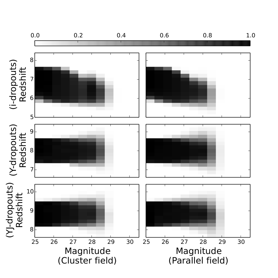
Figure 12 shows the completeness
derived from our simulations.
The left (right) panels indicate the selection windows in the cluster (parallel) field.
At bright magnitudes of mag, our -, -, and -dropout selection criteria
provide a high completeness sample of star-forming galaxies at
, , and , respectively.
V.3. Best-fit Schechter Parameters of UV Luminosity Functions
These completeness estimates are then used to predict observed galaxy number counts. We calculate the predicted number counts from the completeness estimates and a UV luminosity function expressed as a Schechter function with a set of parameters, (, , ), and repeat it for various sets of Schechter parameters covering a wide parameter space. In this way, we obtain the predicted number counts for various sets of Schechter parameters. Because the completeness values are estimated with all of the observational effects in the image plane, these predicted number counts include the lensing magnifications, magnification, distortion, and multiplication as well as the corresponding detection incompleteness in the redshift and magnitude space.
Using the predicted number counts, we search for the best-fit Schechter parameters that reproduce the observed number counts of our dropout candidates. We adopt a maximum likelihood method, assuming a Poisson distribution of the number counts. The likelihood is written as
| (29) |
where is the expected number counts from a given Schechter function in a magnitude interval and is the observed number counts in the magnitude interval. Constraining the Schechter parameters, we simultaneously fit both the observed HFF number counts and the UV luminosity function data points obtained in the previous studies. For our dropouts at , we compare our number counts of with the luminosity function data points of in previous studies, assuming that the UV luminosity function does not rapidly change in . We take the previous blank-field survey results from the studies of CANDELS, HUDF09, HUDF12, ERS, and BORG/HIPPIES (Bouwens et al. 2014), UltraVISTA+UKIDSS UDS (Bowler et al. 2014), BoRG (Bradley et al. 2012), SDF+GOODS-N (Ouchi et al. 2009), and HUDF12/XDF+CANDELS (Oesch et al. 2013). We regard , , and as free parameters for the fitting of number counts at and . Because the statistics of the luminosity function is poor, we choose for a free parameter and and to be fixed to the best-fit values of . Maximizing the Poisson likelihood, we obtain the best-fit parameters of for the dropout candidates, for the dropout candidates, and for the dropout candidates. Table 7 summarizes these parameters, together with those obtained by the previous studies. We find that our results are consistent with the previous results within the uncertainties. Figures 13 and show the confidence intervals on the versus plane for the UV luminosity functions at and , respectively. To test our results, we also perform Schechter function fittings without the results from the HUDF09+ERS data at and . We confirm that the fitting results without the HUDF09+ERS data are consistent with the previous results, although the uncertainties are substantially large due to the small statistics of the HFF samples.
| Reference | [Mpc-3] | ||
|---|---|---|---|
| This Work | |||
| Atek et al. (2014a) | |||
| Bouwens et al. (2014) | |||
| Bouwens et al. (2011) | |||
| Ouchi et al. (2009) | |||
| Schenker et al. (2013) | |||
| This Work | |||
| Bouwens et al. (2014) | |||
| Bouwens et al. (2011) | |||
| Bradley et al. (2012) | |||
| Schenker et al. (2013) | |||
| This Work | (fixed) | (fixed) | |
| Oesch et al. (2013) | (fixed) | (fixed) | |
| Bouwens et al. (2012) | (fixed) | (fixed) | |
The top and bottom panels of Figures 14-16 present the best-fitting number counts and Schechter functions, respectively. In the bottom panels, we present recent studies of and luminosity functions, Schenker et al. (2013), Finkelstein et al. (2014), and Atek et al. (2014a) for comparison. The best-fitting results broadly agree with the observed number counts. The observed number counts of at the bright end are larger than the best-fit function. It is probably caused by the field-to-field variance, since our effective survey area is only arcmin2 in the source plane. In fact, eight of the dropouts are found within a small region with a radius of (corresponding to a physical length of kpc at ). This overdensity of dropouts is originally claimed by Zheng et al. (2014) with the early optical images shallower than our full-depth data by magnitudes. Because one cannot remove a number of foreground interlopers with the shallow early optical data, the existence of overdensity is open question (see the discussion in Coe et al. 2014). In our study with the full-depth HFF data deep enough to remove such foreground interlopers reliably, there is the overdensity of dropouts, indicative that the overdensity is real. If it is true, the existence of the overdensity would significantly enhance the source number counts of dropouts at in the HFF fields.
The middle panels of Figures 14-16 show the histograms of the numbers of dropout galaxies used for the UV luminosity function determinations. We also show the numbers of dropout galaxies newly identified in the observations of the HDF12 at (Schenker et al. 2013) and those of CLASH at (Bouwens et al. 2012). These histograms indicate that our HFF samples enable us to probe the UV luminosity functions down to a faint UV magnitude of , which is comparable to survey limits of the deepest blank-field observations of the HUDF (Ellis et al. 2013; Oesch et al. 2013), thanks to the gravitational lensing effects. In addition to the lensing effects, the HFF Abell 2744 observations provide two new ultra-deep imaging regions of the cluster and parallel fields, allowing us to significantly increase the number of dropouts (cf. the dropout samples in UDF12 and CANDELS Oesch et al. 2013).
VI. Discussion
In Section V, we have derived the UV luminosity functions of dropout galaxies at , , and based on our HFF and the previous study data. We improve the faint-end luminosity function determinations with the large samples extending the magnitude range. The UV luminosity functions are tightly connected with the production rates of ionizing photons escaping to the IGM, which are important observational quantities to understand the process of cosmic reionization, In this section, we carry out the joint analysis of the UV luminosity functions and the electron scattering optical depth measured by the CMB observations to discuss the ionizing sources of the IGM.
VI.1. Evolution of the UV Luminosity Density
To investigate the ionizing sources for the cosmic reionization, we first estimate UV luminosity densities from our UV luminosity functions. is calculated by
| (30) |
where is the truncation magnitude of the UV luminosity function where no galaxies exist beyond this magnitude. Because the parameter is not constrained by observations, in this study we assume two values that bracket the plausible range of the parameter; mag corresponding to the current observational limit and mag being the predicted magnitude of minimum-mass halos that can host star-forming galaxies (Faucher-Giguère et al. 2011).
We use the best-fit Schechter functions shown in Section V and those in the literature for (Bouwens et al. 2007), (Bouwens et al. 2012), and (Bouwens et al. 2014). For comparison purpose, we plot the data for taken from Schenker et al. (2013) and McLure et al. (2013). Because the data of Schenker et al. (2013) and McLure et al. (2013) are included in our luminosity function estimates via Bouwens et al. (2014) data points, we do not use these data points of Schenker et al. (2013) and McLure et al. (2013) for fitting analyses carried out in Section VI.2. The top and bottom left panels of Figure 17 present the as a function of redshift under the assumptions of and , respectively. The solid and dashed lines show the best-fit functions of with two fitting methods detailed in Section VI.2. We confirm that our at are broadly consistent with the previous results, and that there is a rapid decrease of from towards high redshifts, which is claimed by Oesch et al. (2013) and Bouwens et al. (2014). With the improved measurements of in our study, this trend of the rapid decrease is strengthened. To test whether the rapid decrease is confirmed with the HFF data alone, we derive the luminosity function at with the HFF data alone, and estimate at . The gray circles in the left panels of Figure 17 indicate obtained with our HFF data alone. Although the uncertainty is large, the HFF data independently support the rapid decrease of from . Similar analysis is found in Oesch et al. (2014). They derive the luminosity function at from the HFF cluster data alone. we plot at calculated from the luminosity function derived by Oesch et al. (2014) with the gray squares. These plots are also consistent with the rapid decrease from .
Robertson et al. (2014) estimate the cosmic variance uncertainties of the high-redshift galaxies in the Abell 2744 cluster field. The uncertainties are at and at . Our errors of slightly increase by the cosmic variance uncertainties. However, our conclusion does not change because our at is smaller than at by a factor of two, which is significantly larger than the uncertainties of the cosmic variance.
VI.2. Properties of the Ionizing Sources Revealed from the and Measurements
The evolution of the ionized hydrogen fraction in the IGM, , is described by the following ionization equation (e.g., Robertson et al. 2013),
| (31) |
where the dots denote time derivatives.
The first term in the right-hand side of Equation (31) is a source term proportional to the ionizing photon emissivity. and are the production rate of ionizing photons and the mean hydrogen number density, respectively. They are defined by
| (32) | |||||
| (33) |
is the primordial mass fraction of hydrogen, is the critical density, and is the mass of the hydrogen atom. Note that and are parameters that appear in the product form for our analysis. If one assumes that and depend on , is a magnitude-averaged value defined in Equation (32).
The second term in the right-hand side of Equation (31) is a sink term due to recombinations; is the averaged gas recombination time,
| (34) |
where is the case B hydrogen recombination coefficient, and is the IGM temperature at a mean density. is the primordial helium mass fraction. Substituting Equations (32)-(34) into Equation (31), we obtain
| (35) | |||||
| (36) | |||||
| (37) |
Once the evolution of is determined by these equations, at a redshift is estimated (e.g., Kuhlen & Faucher-Giguère 2012) from
| (38) |
where is the speed of light, is the Hubble parameter, and is the Thomson scattering cross section. We assume that helium is singly ionized () at and doubly ionized () at (Kuhlen & Faucher-Giguère 2012). The value of is measured to be (Planck Collaboration et al. 2013) from the combination of the Planck temperature power spectrum, the WMAP polarization low-multipole () likelihood (Bennett et al. 2013), and the high-resolution ground-based CMB data (e.g., Reichardt et al. 2012, Story et al. 2013).
We assume that is approximated by a logarithmic double power law,
| (39) |
where is a normalization factor, and and determine the slopes of . This double power-law function recovers the rapid decrease of from towards high redshifts.
With the analytic reionization models described with Equations (35)-(39), we carry out fitting to the observational data of and to search for reionization models allowed by these observational constraints. There are six free parameters in the fit, , , , , and . Because there is no observational data point of at , we extrapolate the best-fit function of to . At , we assume . In conjunction with this assumption, we regard that should agree with the value from the CMB measurements.
For the data of in the fitting, we use all of the data points presented in Figure 17 (Section VI.1), except for those given by Schenker et al. (2013) and McLure et al. (2013) at and . Note that the data from these two studies are already included in our estimates via our best-fit UV luminosity functions in Section V.3. We, thus, use a total of 8 data points for the fitting.
The fitting ranges of and are and , respectively. The range of is motivated by the estimate of spectral properties of high-redshift galaxies in Robertson et al. (2013). We calculate the value by simply summing up the value of each data point of and , and obtain the best-fitting parameters. We refer to this fitting method as a simple (SC) method.
From the minimization of the SC method, we find the best-fit parameters for and . The best-fit parameters and the values are shown in Table 8. Figure 18 presents values on the versus plane calculated by the SC method. is determined by , where is the minimum value. In Figure 17, we show the best-fit functions of and for and . Figure 17 indicates that the best-fit agrees with the data points, but that the best-fit is significantly lower than the one of the CMB measurement. The values and the degrees of freedom (dof) shown in Table 8 suggest that the probabilities of these values occurring by chance are and with and , respectively. It indicates that our analytic reionization models may not be good enough to explain the reionization history and sources of reionization.
The best-fit functions by the SC method are weighted by the data more strongly than the data, because the number of data points of is 8, while that of is 1. Here, we calculate values by another method which gives equal weight to and data sets. In this method, we divide the values of the data by 8, that is the number of the data points. We refer to this method as an equally-weighted (EWC) method. The best-fit parameters and functions by the EWC method are shown in Table 8 and Figure 17, respectively. In the case of EWC, the best-fit falls in the error range of the CMB measurement as we expect. However, there is a discrepancy between the best-fit and the observational data points especially at where the observational data exhibit the rapid decrease towards high-.
Even if we change the weights of the fitting and allow the large parameter space of and , we have found that no single model can reproduce both the and data points from the observations. This is because the data points of decrease too rapidly at to contribute to adding . This conclusion is in contrast with the claims of the pioneering study of Robertson et al. (2013) who find a parameter space of the similar analytic models explaining the observational and data available in 2013. While the best measurement value of is almost unchanged since then, the rapid decrease of at is clearly identified by the subsequent observational studies including our HFF work. The strong constraints on the evolution of at probably allow us to find the discrepancy between the analytic models and the observational data.
| log | dof | ||||||
|---|---|---|---|---|---|---|---|
| (log erg-1 Hz) | (log ) | ||||||
| SC method | |||||||
| EWC method | |||||||
There are three possible explanations for the discrepancy between the models and the observational data of and . First, the decrease of at may not be as rapid as that found at . Because there is no data at , in our model we extrapolate the best-fit power-law of towards . If the real values at are larger than this extrapolation, the value becomes larger, which eases the tension between the model prediction and the observations. The slow decrease of at may be made by a fainter than mag and/or a luminosity function slope () steeper than the values found at (Table 7). In other words, the discrepancy that we find may suggest that faint galaxies dominate at even more than at . It is also possible that the rapid decrease would be weakened by the luminosity function slope steepening and/or becoming fainter at . Second, the evolution of or can increase , such suggested by Kuhlen & Faucher-Giguère (2012). If the value becomes large towards high-, (accordingly ) could be boosted. Similarly, the small would enhance , although can be as low as unity by definition. Third, another source of ionizing photons besides massive stars of galaxies may exist, which contributes to the cosmic reionization significantly. X-ray sources such as X-ray binaries and faint AGNs would not leave a clear signature in the measurements, but provide a fraction of ionizing photons via X-ray necessary for the cosmic reionization (Fragos et al. 2013; Madau et al. 2004; Mesinger et al. 2013).
The bottom right panel of Figure 17 shows as a function of redshift, reproduced by our best-fit models. In Figure 17, we also plot estimated from observational results of the Ly forest transmission (Mesinger 2010; McGreer et al. 2011), Ly near-zone sizes around high-redshift quasars (Carilli et al. 2010; Bolton et al. 2011), Ly damping wing absorption in a GRB spectrum (Totani et al. 2006; McQuinn et al. 2008), evolution of the Ly luminosity function and Ly emitter clustering (Ota et al. 2008; Ouchi et al. 2010; Konno et al. 2014), and the Ly emitting galaxy fraction evolution (Pentericci et al. 2011; Schenker et al. 2012; Ono et al. 2012). Because these measurements have uncertainties too large to constrain our model parameters, we do not use these measurements for our model fitting. However, Figure 17 illustrates that our best-fit models are in good agreement with most of the measurements.
VII. Summary
We conduct the comprehensive analyses of the full-depth HFF Abell 2744 cluster and parallel field data whose observations completed in July 2014, and study faint dropout galaxies at . We construct a mass model for Abell 2744 to evaluate the gravitational lensing effects of the cluster. Then we estimate number densities of our dropout candidates with realistic Monte-Carlo simulations in the image plane including detection completeness, contamination, and all lensing effects such as magnification, distortion, and multiplication of images.
The major results of our study are as follows.
- 1.
We identify dropout candidates at with the -, -, and -dropout selection criteria. The magnifications of our dropout candidates range from to . The intrinsic magnitudes of our dropout candidates reach mag that is comparable to survey limits of the deepest blank-field observations of the HUDF.
- 2.
The number densities of our dropout candidates are consistent with previous results of blank-field surveys. However, we find a slight excess of the number of our bright dropout candidates at probably due to field-to-field variance.
- 3.
We derive the UV luminosity functions at , , and combining our HFF results with the previous blank-field surveys. We confirm that the faint-end slopes of the luminosity functions () are as steep as both at and . The number of dropout candidates at increases significantly by our HFF study, and strengthen the early claim of the rapid decrease from to from the evolution of .
- 4.
We use the simple analytic reionization models to explain the observational results of the evolution and the CMB’s . None of our models can reproduce both of these observational measurements, due to the rapid decrease of and the large value, even if we allow a large parameter space of , , and . This problem could be resolved by the slow decrease of at , the evolution of and/or , or another source of reionization such as X-ray bright populations of X-ray binaries and faint AGN.
The HFF program will provide a significantly large sample of high-redshift galaxies when the observations of the planned six clusters are completed. In the Abell 2744 cluster field, we find 3 dropout candidates whose magnifications are . A simple scaling suggests that the complete HFF observations will provide highly-magnified () systems at high redshift, which will uncover the properties of the faint galaxies at the epoch of cosmic reionization and greatly improve our understanding of sources of reionization up to .
References
- Atek et al. (2014a) Atek, H., Richard, J., Kneib, J.-P., et al. 2014a, ArXiv e-prints, arXiv:1409.0512
- Atek et al. (2014b) —. 2014b, ApJ, 786, 60
- Benítez (2000) Benítez, N. 2000, ApJ, 536, 571
- Benitez-Llambay et al. (2014) Benitez-Llambay, A., Navarro, J. F., Abadi, M. G., et al. 2014, ArXiv e-prints, arXiv:1405.5540
- Bennett et al. (2013) Bennett, C. L., Larson, D., Weiland, J. L., et al. 2013, ApJS, 208, 20
- Bertin & Arnouts (1996) Bertin, E., & Arnouts, S. 1996, A&AS, 117, 393
- Bertin et al. (2002) Bertin, E., Mellier, Y., Radovich, M., et al. 2002, in Astronomical Society of the Pacific Conference Series, Vol. 281, Astronomical Data Analysis Software and Systems XI, ed. D. A. Bohlender, D. Durand, & T. H. Handley, 228
- Bolton et al. (2011) Bolton, J. S., Haehnelt, M. G., Warren, S. J., et al. 2011, MNRAS, 416, L70
- Bouwens et al. (2012) Bouwens, R., Bradley, L., Zitrin, A., et al. 2012, ArXiv e-prints (arXiv:1211.2230), arXiv:1211.2230
- Bouwens et al. (2007) Bouwens, R. J., Illingworth, G. D., Franx, M., & Ford, H. 2007, ApJ, 670, 928
- Bouwens et al. (2011) Bouwens, R. J., Illingworth, G. D., Oesch, P. A., et al. 2011, ApJ, 737, 90
- Bouwens et al. (2014) —. 2014, ArXiv e-prints, arXiv:1403.4295
- Bowler et al. (2014) Bowler, R. A. A., Dunlop, J. S., McLure, R. J., et al. 2014, MNRAS, 440, 2810
- Boylan-Kolchin et al. (2014) Boylan-Kolchin, M., Bullock, J. S., & Garrison-Kimmel, S. 2014, ArXiv e-prints, arXiv:1405.1040
- Bradley et al. (2012) Bradley, L. D., Trenti, M., Oesch, P. A., et al. 2012, ApJ, 760, 108
- Bradley et al. (2013) Bradley, L. D., Zitrin, A., Coe, D., et al. 2013, ArXiv e-prints, arXiv:1308.1692
- Carilli et al. (2010) Carilli, C. L., Wang, R., Fan, X., et al. 2010, ApJ, 714, 834
- Coe et al. (2014) Coe, D., Bradley, L., & Zitrin, A. 2014, ArXiv e-prints, arXiv:1405.0011
- Dijkstra et al. (2011) Dijkstra, M., Mesinger, A., & Wyithe, J. S. B. 2011, MNRAS, 414, 2139
- Ellis et al. (2013) Ellis, R. S., McLure, R. J., Dunlop, J. S., et al. 2013, ApJ, 763, L7
- Fan et al. (2006) Fan, X., Carilli, C. L., & Keating, B. 2006, ARA&A, 44, 415
- Faucher-Giguère et al. (2011) Faucher-Giguère, C.-A., Kereš, D., & Ma, C.-P. 2011, MNRAS, 417, 2982
- Finkelstein et al. (2013) Finkelstein, S. L., Papovich, C., Dickinson, M., et al. 2013, Nature, 502, 524
- Finkelstein et al. (2014) Finkelstein, S. L., Ryan, Jr., R. E., Papovich, C., et al. 2014, ArXiv e-prints, arXiv:1410.5439
- Fragos et al. (2013) Fragos, T., Lehmer, B. D., Naoz, S., Zezas, A., & Basu-Zych, A. 2013, ApJ, 776, L31
- Hinshaw et al. (2013) Hinshaw, G., Larson, D., Komatsu, E., et al. 2013, ApJS, 208, 19
- Jaacks et al. (2013) Jaacks, J., Thompson, R., & Nagamine, K. 2013, ApJ, 766, 94
- Jaffe (1983) Jaffe, W. 1983, MNRAS, 202, 995
- Jauzac et al. (2014) Jauzac, M., Richard, J., Jullo, E., et al. 2014, ArXiv e-prints, arXiv:1409.8663
- Johnson et al. (2014) Johnson, T. L., Sharon, K., Bayliss, M. B., et al. 2014, ArXiv e-prints (arXiv:1405.0222), arXiv:1405.0222
- Kashikawa et al. (2006) Kashikawa, N., Shimasaku, K., Malkan, M. A., et al. 2006, ApJ, 648, 7
- Kashikawa et al. (2011) Kashikawa, N., Shimasaku, K., Matsuda, Y., et al. 2011, ApJ, 734, 119
- Keeton (2001) Keeton, C. R. 2001, ArXiv Astrophysics e-prints (astro-ph/0102341), astro-ph/0102341
- Kochanek (1991) Kochanek, C. S. 1991, ApJ, 373, 354
- Konno et al. (2014) Konno, A., Ouchi, M., Ono, Y., et al. 2014, ArXiv e-prints, arXiv:1404.6066
- Kron (1980) Kron, R. G. 1980, ApJS, 43, 305
- Kuhlen & Faucher-Giguère (2012) Kuhlen, M., & Faucher-Giguère, C.-A. 2012, MNRAS, 423, 862
- Lam et al. (2014) Lam, D., Broadhurst, T., Diego, J. M., et al. 2014, ArXiv e-prints, arXiv:1406.2702
- Laporte et al. (2014) Laporte, N., Streblyanska, A., Clement, B., et al. 2014, A&A, 562, L8
- Madau et al. (1996) Madau, P., Ferguson, H. C., Dickinson, M. E., et al. 1996, MNRAS, 283, 1388
- Madau et al. (1998) Madau, P., Pozzetti, L., & Dickinson, M. 1998, ApJ, 498, 106
- Madau et al. (2004) Madau, P., Rees, M. J., Volonteri, M., Haardt, F., & Oh, S. P. 2004, ApJ, 604, 484
- McGreer et al. (2011) McGreer, I. D., Mesinger, A., & Fan, X. 2011, MNRAS, 415, 3237
- McLure et al. (2013) McLure, R. J., Dunlop, J. S., Bowler, R. A. A., et al. 2013, MNRAS, 432, 2696
- McQuinn et al. (2007) McQuinn, M., Hernquist, L., Zaldarriaga, M., & Dutta, S. 2007, MNRAS, 381, 75
- McQuinn et al. (2008) McQuinn, M., Lidz, A., Zaldarriaga, M., Hernquist, L., & Dutta, S. 2008, MNRAS, 388, 1101
- Mesinger (2010) Mesinger, A. 2010, MNRAS, 407, 1328
- Mesinger et al. (2013) Mesinger, A., Ferrara, A., & Spiegel, D. S. 2013, MNRAS, 431, 621
- Mesinger & Furlanetto (2008) Mesinger, A., & Furlanetto, S. R. 2008, MNRAS, 386, 1990
- Meurer et al. (1999) Meurer, G. R., Heckman, T. M., & Calzetti, D. 1999, ApJ, 521, 64
- Montes & Trujillo (2014) Montes, M., & Trujillo, I. 2014, ArXiv e-prints, arXiv:1405.2070
- Nakamura & Suto (1997) Nakamura, T. T., & Suto, Y. 1997, Progress of Theoretical Physics, 97, 49
- Navarro et al. (1997) Navarro, J. F., Frenk, C. S., & White, S. D. M. 1997, ApJ, 490, 493
- Oesch et al. (2014) Oesch, P. A., Bouwens, R. J., Illingworth, G. D., et al. 2014, ArXiv e-prints, arXiv:1409.1228
- Oesch et al. (2010) Oesch, P. A., Bouwens, R. J., Carollo, C. M., et al. 2010, ApJ, 709, L21
- Oesch et al. (2013) Oesch, P. A., Bouwens, R. J., Illingworth, G. D., et al. 2013, ApJ, 773, 75
- Oguri (2010) Oguri, M. 2010, PASJ, 62, 1017
- Ono et al. (2012) Ono, Y., Ouchi, M., Mobasher, B., et al. 2012, ApJ, 744, 83
- Ono et al. (2013) Ono, Y., Ouchi, M., Curtis-Lake, E., et al. 2013, ApJ, 777, 155
- Ota et al. (2008) Ota, K., Iye, M., Kashikawa, N., et al. 2008, ApJ, 677, 12
- Ouchi et al. (2004) Ouchi, M., Shimasaku, K., Okamura, S., et al. 2004, ApJ, 611, 660
- Ouchi et al. (2009) Ouchi, M., Mobasher, B., Shimasaku, K., et al. 2009, ApJ, 706, 1136
- Ouchi et al. (2010) Ouchi, M., Shimasaku, K., Furusawa, H., et al. 2010, ApJ, 723, 869
- Owers et al. (2011) Owers, M. S., Randall, S. W., Nulsen, P. E. J., et al. 2011, ApJ, 728, 27
- Pentericci et al. (2011) Pentericci, L., Fontana, A., Vanzella, E., et al. 2011, ApJ, 743, 132
- Pentericci et al. (2014) Pentericci, L., Vanzella, E., Fontana, A., et al. 2014, ArXiv e-prints, arXiv:1403.5466
- Planck Collaboration et al. (2013) Planck Collaboration, Ade, P. A. R., Aghanim, N., et al. 2013, ArXiv e-prints, arXiv:1303.5076
- Ravindranath et al. (2006) Ravindranath, S., Giavalisco, M., Ferguson, H. C., et al. 2006, ApJ, 652, 963
- Reichardt et al. (2012) Reichardt, C. L., Shaw, L., Zahn, O., et al. 2012, ApJ, 755, 70
- Richard et al. (2014) Richard, J., Jauzac, M., Limousin, M., et al. 2014, ArXiv e-prints, arXiv:1405.3303
- Robertson et al. (2010) Robertson, B. E., Ellis, R. S., Dunlop, J. S., McLure, R. J., & Stark, D. P. 2010, Nature, 468, 49
- Robertson et al. (2014) Robertson, B. E., Ellis, R. S., Dunlop, J. S., et al. 2014, ArXiv e-prints, arXiv:1410.0962
- Robertson et al. (2013) Robertson, B. E., Furlanetto, S. R., Schneider, E., et al. 2013, ApJ, 768, 71
- Schenker et al. (2014) Schenker, M. A., Ellis, R. S., Konidaris, N. P., & Stark, D. P. 2014, ArXiv e-prints, arXiv:1404.4632
- Schenker et al. (2012) Schenker, M. A., Stark, D. P., Ellis, R. S., et al. 2012, ApJ, 744, 179
- Schenker et al. (2013) Schenker, M. A., Robertson, B. E., Ellis, R. S., et al. 2013, ApJ, 768, 196
- Story et al. (2013) Story, K. T., Reichardt, C. L., Hou, Z., et al. 2013, ApJ, 779, 86
- Tody (1986) Tody, D. 1986, in Society of Photo-Optical Instrumentation Engineers (SPIE) Conference Series, Vol. 627, Instrumentation in astronomy VI, ed. D. L. Crawford, 733
- Tody (1993) Tody, D. 1993, in Astronomical Society of the Pacific Conference Series, Vol. 52, Astronomical Data Analysis Software and Systems II, ed. R. J. Hanisch, R. J. V. Brissenden, & J. Barnes, 173
- Totani et al. (2006) Totani, T., Kawai, N., Kosugi, G., et al. 2006, PASJ, 58, 485
- Totani et al. (2013) Totani, T., Aoki, K., Hattori, T., et al. 2013, ArXiv e-prints, arXiv:1312.3934
- Treu et al. (2013) Treu, T., Schmidt, K. B., Trenti, M., Bradley, L. D., & Stiavelli, M. 2013, ApJ, 775, L29
- Weisz et al. (2014) Weisz, D. R., Dolphin, A. E., Skillman, E. D., et al. 2014, ArXiv e-prints, arXiv:1405.3281
- Yagi et al. (2002) Yagi, M., Kashikawa, N., Sekiguchi, M., et al. 2002, AJ, 123, 66
- Zheng et al. (2014) Zheng, W., Shu, X., . Moustakas, J., et al. 2014, ArXiv e-prints (arXiv:1402.6743), arXiv:1402.6743
- Zitrin et al. (2014) Zitrin, A., Zheng, W., Broadhurst, T., et al. 2014, ArXiv e-prints, arXiv:1407.3769