Quantum de Finetti theorem under fully-one-way adaptive measurements

Consider random variables $X_{1},...,X_{n}$ representing the color of a sequence of balls drawn without replacement from a bag of $100$ red balls and $100$ blue balls. These variables are not independent, since the probability of withdrawing a red ball on the $k$th withdrawl depends on the number of balls of each color remaining. They are, however, exchangeable: the probability of removing a particular sequence of balls $(x_{1},...,x_{n})$ is equal to the probability of removing any reordering of that sequence $(x_{\pi(1)},...,x_{\pi(n)})$ for permuatation $\pi$. Remarkably, the de Finetti theorem tells us that any such exchangeable random variables can be represented by independent and identically distributed ones [1, 2], yeilding a profound result in probability theory and a powerful tool in statistics.

A series of works have established analogues of this theorem in the quantum domain [3, 4, 5, 6, 7, 8, 9, 10], where a classical probability distribution is replaced by a quantum state and the situation is more complicated and interesting, due to entanglement and the existence of many different ways to distinguish states of multipartite systems. These quantum de Finetti theorems are appealing not only due to their own elegance on the characterization of symmetric states, but also because of the successful applications in many-body physics [5, 11, 12], quantum information [9, 13, 14], and computational complexity theory [15, 16, 10].

More precisely, a quantum de Finetti theorem concerns the structure of a symmetric state $\rho_{A_{1}\ldots A_{n}}$ that is invariant under any permutations over the subsystems [17]. It tells how the reduced state $\rho_{A_{1}\ldots A_{k}}$ on a smaller number $k<n$ of subsystems could be approximated by a mixture of $k$-fold product states, namely, de Finetti states of the form $\int\sigma^{\otimes k}\,\mathrm{d}\mu(\sigma)$. Here $\mu$ is a probability measure over density matrices. Using the conventional distance measure, trace norm, Ref. [8] proved a standard de Finetti theorem with an essentially optimal error bound $2|A|^{2}k/n$ for the approximation ($|A|$ denotes the dimension of the subsystems). However, in many situations this bound is too large to be applicable. Luckily it is possible to circumvent this obstruction. For example, Renner’s exponential de Finetti theorem employs the “almost” de Finetti states and has an error bound that decreases exponentially in $n-k$ [9], being very useful in dealing with cryptography or information theory problems [9, 13, 14].

In a beautiful work [10] Brandão and Harrow recently proved an LOCC (local operations and classical communication) de Finetti theorem, generalizing a similar result for the case $k=2$ [16]. Both [10] and [16] have overcome the limitation of the standard de Finetti theorem regarding the dimension dependence. The basic idea is to relax the measure of approximation by replacing the trace norm with a kind of one-way LOCC norm. This gives an error bound $\sqrt{\frac{2k^{2}\ln|A|}{n-k}}$ [18], scaling polynomially in $\ln|A|$ instead of polynomially in $|A|$ as in earlier de Finetti results, which is crucial to the complexity-theoretic applications.

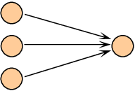
While [10] showed approximation in the parallel one-way LOCC norm associated with the measurement class $\mathsf{LOCC_{1}^{\parallel}}$, here we prove a de Finetti theorem where the approximation is measured with the fully one-way LOCC norm (or relative entropy) associated with $\mathsf{LOCC_{1}}$ (cf. Fig. 1). The error bound remains essentially the same as that of [10]. This improves Brandão and Harrow’s LOCC de Finetti theorem considerably: it is conceptually more complete and when applied to the problems considered in [16, 19, 10] gives new and improved results. For the problem of entanglement detection, so central to quantum information theory and experiment, we present strong guarantees for the effectiveness of the well-known heirarchy of entanglement tests of [20]. We also consider the power of multiple-prover quantum Merlin Arthur games, which bears directly on the problems of pure-state vs mixed-state $N$-representability [21] as well as the entanglement properties of sparse hamiltonian’s ground states [22].

In the proof, we will use information-theoretic methods similar to [10], along with some new ideas. In particular, Lemma 2 presented below is a crucial new technical tool, which may be of independent interest. We employ and manipulate entropic quantities to derive the final result: apart from relative entropy, the mutual information of a state $\omega_{AB}$ is defined as $I(A;B):=D(\omega_{AB}\|\omega_{A}\otimes\omega_{B})$, and the conditional mutual information of a state $\omega_{ABC}$ is defined as $I(A;B|C):=I(A;BC)-I(A;C)$.

Group the $n$ subsystems as shown in Fig. 2: except for one subsystem, the others are divided into groups of $k-1$ subsystems each (we discard the possibly remaining qubits, of which there will be fewer than $k-1$). So, we have $m=\lfloor\frac{n-1}{k-1}\rfloor\geq\frac{n-k}{k-1}$ groups. Label the groups as bigger subsystems $B_{1},B_{2},\ldots,B_{m}$ and the isolated system as $A$. Let the $k-1$ subsystems in $B_{1}$ be $A_{1},A_{2},\ldots,A_{k-1}$ and the system $A$ is also identified with $A_{k}$.

Obviously the total state is invariant under permutations over $B_{1},B_{2},\ldots,B_{m}$. So Lemma 3 applies. Thus there exists a measurement $\mathcal{Q}^{*}:B_{2}\ldots B_{m}\rightarrow X$, such that for any measurement $\mathcal{P}:B_{1}\rightarrow Y$ we have

$\mathcal{Q}^{*}$ effectively decomposes the state on $AB_{1}$ into an ensemble. Specifically, we have $\rho_{AB_{1}}=\sum_{x}p_{x}\rho_{A_{1}\ldots A_{k}}^{x}$, where $p_{x}$ is the probability of obtaining the measurement outcome $x$ and $\rho_{A_{1}\ldots A_{k}}^{x}$ is the resulting state on $A_{1}\ldots A_{k}$. Note that since $\rho_{A_{1}\ldots A_{n}}$ is permutation-invariant, the post-measurement states $\rho_{A_{1}\ldots A_{k}}^{x}$ are also permutation-invariant. Now we rewrite Eq. (3) in terms of the relative entropy: for any measurement $\mathcal{P}$ on $A_{1}\ldots A_{k-1}$,

Pick a one-way LOCC measurement $\Lambda^{k}$ acting on systems $A_{1},\ldots,A_{k}$ and denote its reduced measurement on the first $\ell$ systems as $\Lambda^{\ell}$. Now we apply Lemma 2 to each state $\rho_{A_{1}\ldots A_{k}}^{x}$ and get

where for the first inequality we have also applied the monotonicity of relative entropy [26] and for the second inequality we used the monotonicity of relative entropy again as well as the symmetry of the state $\rho_{A_{1}\ldots A_{k}}^{x}$. Combining Eq. (4) and Eq. (5) we arrive at

where the first inequality is due to the joint convexity of relative entropy. At this point we are able to conclude Eq. (1) from Eq. (6), noticing that $\Lambda^{k}\in\mathsf{LOCC_{1}}$ is picked arbitrarily and $\sum_{x}p_{x}\rho_{A_{1}}^{x}\otimes\ldots\otimes\rho_{A_{k}}^{x}$ is a de Finetti state of the form $\sum_{x}p_{x}(\rho_{A}^{x})^{\otimes k}$ due to the symmetry of $\rho_{A_{1}\ldots A_{k}}^{x}$.   $\sqcap$$\sqcup$

The following lemma, which is a statement of the monogamy of entanglement, is adapted from [10]. For completeness we give a proof in the Appendix.

We consider the situation where a small error $\epsilon$ is permitted, meaning that we must detect all the entangled states except for those very weak ones that are $\epsilon$-close to separable (at the same time all the separable states should be detected correctly). This is equivalently formulated as the Weak Membership Problem for separability: given a state $\rho_{A_{1}A_{2}\ldots A_{k}}$ that is either separable or $\epsilon$-away from any separable state, we want to decide which is the case. It has been shown that this problem is ${\mathsf{NP}}$-hard when $\epsilon$ is of the order no larger than inverse polynomial of local dimensions (in trace norm) [28, 29, 30]. Surprisingly, Brandão, Christandl and Yard found a quasipolynomial-time algorithm for constant $\epsilon$ in one-way LOCC norm for bipartite states [16]. This algorithm was generalized to multipartite states in [19], then in [10] using a stronger method. These algorithms are all based on the searching for symmetric extensions of [20]. Along these lines, we present the following result, which is obtained by applying Theorem 1 to bound the distance between properly extendible states and separable states.

It is worth mentioning that the run time in Eq. (10) is quasipolynomial, for constant particle number $k$ and constant error $\epsilon$. The algorithm in [19] using $\mathsf{LOCC_{1}}$-norm behaves exponentially slower than ours with respect to the number of particles $k$, while the algorithm of [10] has the same run-time as ours but works only for $\mathsf{LOCC_{1}^{\parallel}}$-norm rather than our $\mathsf{LOCC_{1}}$-norm approximation. Thus our result has bridged the gap between these two works. Furthermore, here for the first time we catch the importance of the amount of entanglement in this problem. The quantity $E_{r}^{\mathsf{LOCC_{1}}}(\rho):=\min\{D_{\mathsf{LOCC_{1}}}(\rho\|\sigma):\sigma\text{ being separable}\}$, introduced in [31], is asymptotically normalized since $E_{r}^{\mathsf{LOCC_{1}}}(\Phi_{d})=\log(d+1)-1$ for maximally entangled state $\Phi_{d}$ of local dimension $d$ [32]. Corollary 4 shows that, detecting all the $k$-partite entangled states $\rho$ such that $E_{r}^{\mathsf{LOCC_{1}}}(\rho)\geq\epsilon$ can be done in quasi-polynomial time in local dimensions. This is a stronger statement than using $\mathsf{LOCC_{1}}$-norm as the error measure. We point out that for the bipartite case this result can also be obtained by combining the algorithm of [16] with the “commensurate lower bound” for squashed entanglement of [32].

To solve a problem, the verifier performs a quantum algorithm on the input $x\in\{0,1\}^{n}$ along with the quantum proofs. The algorithm then returns “yes” or “no” as the answer to the instance $x$. This procedure of verification can be effectively described as a set of two-outcome measurements $\{(M_{x},{\openone}-M_{x})\}_{x}$ on the proofs. In the definition below, a problem is formally identified with a “language”.

We are also interested in QMA systems with multiple symmetric proofs. ${\mathsf{SymQMA}}^{{\mathsf{M}}}(k)_{m,c,s}$ is defined in a similar way but here we replace independent proofs $\omega_{1},\ldots,\omega_{k}$ with identical ones $\omega^{\otimes k}$ in both completeness and soundness parts. As a convention, we set ${\mathsf{M}}$ to be ${\mathsf{ALL}}$ (the class of all measurements), $m=poly(n)$, $k=1$, $c=2/3$ and $s=1/3$ as defaults [40]. We can now state our application of Theorem 1 to these complexity classes.

It has been proven in [16] that ${\mathsf{QMA}}={\mathsf{QMA}}^{\mathsf{LOCC_{1}}}(k)$ for constant $k$. Our result generalizes this statement to a polynomial number of proofs. It is also a generalization of the results in [41, 10] which prove the reduction of ${\mathsf{QMA}}^{\mathsf{LO}}(k)$ to ${\mathsf{QMA}}$ ($\mathsf{LO}$ denotes local measurements). On the other hand, Ref. [10] proved that, assuming ETH (exponential time hypothesis for 3-${\mathsf{SAT}}$) [42], any multi-prover QMA protocol with symmetric proofs and Bell verification for 3-${\mathsf{SAT}}$, can not bring better than the square-root reduction of [43] to the proof size. Eq. (12) implies that, this is still true even if adaptively local verification (one-way LOCC measurement) is permitted.

Arguably the biggest open question in the study of QMA proof systems is whether ${\mathsf{QMA}}={\mathsf{QMA}}(2)$ (note that Harrow and Montanaro have proved that ${\mathsf{QMA}}(2)={\mathsf{QMA}}(k)$ for any polynomial $k>2$ [36]). On the one hand, there are natural problems from quantum physics that are in ${\mathsf{QMA}}(2)$ but not obviously in ${\mathsf{QMA}}$ [21, 22, 38]. On the other hand, Harrow and Montanaro showed that if the first equality in Eq. (11) holds for a kind of separable measurements (even only for the case of two proofs), then ${\mathsf{QMA}}={\mathsf{QMA}}(2)$. Our result here, although does not touch this open question directly, is a step towards a larger measurement class compared to [10] and we hope it will stimulate future progress in solving this open question.

We ask whether Theorem 1 can be further improved, to work for two-way LOCC or even separable measurements. This would accordingly give stronger applications, and possibly, solve the ${\mathsf{QMA}}$ vs ${\mathsf{QMA}}(2)$ puzzle due to the result of [36]. Another open question is, for a state supported on the symmetric subspace (aka Bose-symmetric state), whether its reduced states have pure-state approximations of the form $\int\varphi^{\otimes k}\,\mathrm{d}\mu(\varphi)$ with $\varphi$ pure that are not worse than the mixed-state approximations given by our theorem. We notice that this is indeed the case for the de Finetti theorem of [8] and a similar statement holds for [9]. However, our method, as well as that of [10] seems to require that the state $\varphi$ must be generally mixed.

Appendix

To see this, notice that for states of the form $\rho_{ABC}=\rho_{AB}\otimes|0\rangle\!\langle 0|$ and $\sigma_{ABC}=\sigma_{AB}\otimes|0\rangle\!\langle 0|$ we have

where $\mathsf{LO}$ denotes the set of local measurements. We can then apply the existence of bipartite states with $\|\rho_{AB}-\sigma_{AB}\|_{\mathsf{LOCC_{1}}}=2$ and $\|\rho_{AB}-\sigma_{AB}\|_{\mathsf{LO}}\leq C/\sqrt{d}$ as shown in Theorem 2.4 of [24].

Let $\ell\geq k$ be an integer. Introduce quantum systems $\bar{A}_{i}:=A_{1}^{i}A_{2}^{i}\ldots A_{k}^{i}$ with $A_{j}^{i}\cong A_{j}$, for all $0<i\leq\ell$ and $0<j\leq k$. We search for an state $\tilde{\rho}_{\bar{A}_{1}\ldots\bar{A}_{\ell}}$ such that $\tilde{\rho}_{\bar{A}_{1}\ldots\bar{A}_{\ell}}$ is permutation-invariant and $\tilde{\rho}_{A_{1}^{1}A_{2}^{2}\ldots A_{k}^{k}}=\rho_{A_{1}A_{2}\ldots A_{k}}$. If such a state exists, we feed back “separable”. Otherwise we conclude that it is entangled. For our purpose we set $\ell=2(k-1)^{2}\epsilon^{-2}\sum_{i}\ln|A_{i}|+k$.

This search can be done using semidefinite programming in time polynomial of the total dimension of $\tilde{\rho}_{\bar{A}_{1}\ldots\bar{A}_{\ell}}$, which coincides with the claimed result.

To analyze the correctness, first assume that such an extension exists. Then we apply Theorem 1 to see that there is certain probability measure $\mu$ such that

By definition, if we restrict the measurement to be performed only on systems $A_{1}^{1},A_{2}^{2},\ldots,A_{k}^{k}$ then the above inequality implies that there exists a separable state $\sigma_{A_{1}\ldots A_{k}}$ such that $\left\|\rho_{A_{1}\ldots A_{k}}-\sigma_{A_{1}\ldots A_{k}}\right\|_{\mathsf{LOCC_{1}}}\leq\epsilon$. So if $\rho_{A_{1}\ldots A_{k}}$ is $\epsilon$-away from any separable state, the required extension can not exist. But if $\rho_{A_{1}\ldots A_{k}}$ is separable, it is obvious that such an extension does exist. As a result in both cases the above procedure works correctly.

The above argument works as well if the error is measured by the relative entropy. The small modification needed is just to replace $\|\cdot\|_{\mathsf{LOCC_{1}}}$ by $D_{\mathsf{LOCC_{1}}}$ and here we set $\ell=(k-1)^{2}\epsilon^{-1}\sum_{i}\log|A_{i}|+k$.   $\sqcap$$\sqcup$

To prove Eq. (12), we show a way of simulating a ${\mathsf{SymQMA}}^{\mathsf{LOCC_{1}}}(k)_{m,c,s}$ protocol in a single-proof ${\mathsf{QMA}}$ system. The prover provides the verifier with a proof of size $0.6m^{2}k^{2}\epsilon^{-2}$, which consists of $\ell=0.6mk^{2}\epsilon^{-2}$ subsystems each of size $m$ qubits. Then the verifier makes a uniformly random permutation over the subsystems and then performs the ${\mathsf{SymQMA}}^{\mathsf{LOCC_{1}}}(k)_{m,c,s}$ verification on the first $k$ (denoted as $A_{1},A_{2},\ldots,A_{k}$) of them. No matter what the initial state $\rho_{\text{initial}}$ of the proof is, Theorem 1 implies that the state on $A_{1}\ldots A_{k}$, $\rho_{A_{1}\ldots A_{k}}$, can be approximated as $\left\|\rho_{A_{1}\ldots A_{k}}-\int\sigma^{\otimes k}\,\mathrm{d}\mu(\sigma)\right\|_{\mathsf{LOCC_{1}}}\leq 2\epsilon$ with certain probability measure $\mu$. Let $\{(M_{x},{\openone}-M_{x})\}_{x}$ be the one-way LOCC measurements in the ${\mathsf{SymQMA}}^{\mathsf{LOCC_{1}}}(k)_{m,c,s}$ protocol for a language $L$. Then the soundness constant $s^{\prime}$ in this simulation can be

One the other hand, suppose the proof for an accepted instance in ${\mathsf{SymQMA}}^{\mathsf{LOCC_{1}}}(k)_{m,c,s}$ is $\omega^{\otimes k}$. Then in the simulation the state $\omega^{\otimes\ell}$ gives the same probability of acceptance. So completeness does not change.

For Eq. (13), we will prove

This, together with Eq. (12), leads to Eq. (13). The argument is similar to that in [35] (Lemma 38), where the same relation with “$\mathsf{LOCC_{1}}$” replaced by “${\mathsf{ALL}}$” was proved. The strategy is to divide each proof in the ${\mathsf{SymQMA}}^{\mathsf{LOCC_{1}}}(k)_{km,c,s}$ system into $k$ subsystems of $m$ qubits, then simulate the ${\mathsf{QMA}}^{\mathsf{LOCC_{1}}}(k)_{m,c,s}$ protocol on the $i\text{th}$ subsystem from the $i\text{th}$ proof for all $i=1,\ldots,k$.   $\sqcap$$\sqcup$

We use a $d$-dimensional complex vector to encode $2d$ real variables.

References

- [1] B. de Finetti, Ann. Inst. H. Poincare 7, 1 (1937).
- [2] P. Diaconis and D. Freedman, The Annals of Probability 8, 745 (1980).
- [3] E. Størmer, J. Funct. Anal. 3, 48 (1969).
- [4] R. L. Hudson and G. R. Moody, Z. Wahrsch. Verw. Geb. 33, 343 (1976).
- [5] G. A. Raggio and R. F. Werner, Helv. Phys. Acta 62, 980 (1989).
- [6] C. M. Caves, C. A. Fuchs and R. Schack, J. Math. Phys. 43, 4537 (2002).
- [7] R. König and R. Renner, J. Math. Phys. 46, 122108 (2005).
- [8] M. Christandl, R. König, G. Mitchison and R. Renner, Commun. Math. Phys. 273, 473 (2007).
- [9] R. Renner, PhD thesis, ETHZ, Zurich (2005), arXiv:quant-ph/0512258; Nature Phys. 3, 645 (2007).
- [10] F. G. S. L. Brandão and A. W. Harrow, in Proc. of the 45th ACM Symposium on theory of computing (STOC 2013), pp. 861-870 (2013), arXiv:1210.6367.
- [11] M. Fannes and C. Vandenplas, J. Phys. A 39, 13843 (2006).
- [12] M. Lewin, P. T. Nam and N. Rougerie, arXiv:1303.0981.
- [13] F. G. S. L. Brandão and M. B. Plenio, Comm. Math. Phys. 295, 791 (2010).
- [14] M. Christandl and R. Renner, Phys. Rev. Lett. 109, 120403 (2012).
- [15] S. Beigi, P. Shor and J. Watrous, Theory of Computing 7, 101 (2011).
- [16] F. G. S. L. Brandão, M. Christandl and J. Yard, Comm. Math. Phys. 306,805 (2011); Proc. of the 43rd ACM Symposium on theory of computing (STOC 2011), pp. 343–352 (2011); arXiv:1010.1750.
- [17] The exchange of two systems and causes a unitary transformation on their state. We say is permutation-invariant if for any .
- [18] In the present paper, and are logarithms with base and 2, respectively.
- [19] F. G. S. L. Brandão and M. Christandl, Phys. Rev. Lett. 109, 160502 (2012).
- [20] A. C. Doherty, P. A. Parrilo and F. M. Spedalieri, Phys. Rev. Lett. 88, 187904 (2002); Phys. Rev. A 69, 022308 (2004); Phys. Rev. A 71, 032333 (2005).
- [21] Y.-K. Liu, M. Christandl and F. Verstraete, Phys. Rev. Lett. 98, 110503 (2007).
- [22] A. Chailloux and O. Sattath, in Proc. of IEEE 27th Annual Conference on Computational Complexity (CCC), pp 32 – 41 (2012).
- [23] W. Matthews, S. Wehner and A. Winter, Comm. Math. Phys. 291,813 (2009).
- [24] G. Aubrun and C. Lancien, arXiv:1406.1959.
- [25] C. A. Fuchs and J. van de Graaf, IEEE. Tran. Inf. Theory 45, 1216 (1999).
- [26] G. Lindblad, Comm. Math. Phys. 40, 147 (1975); A. Uhlmann, Comm. Math. Phys. 54, 21 (1977).
- [27] R. Horodecki, P. Horodecki, M. Horodecki and K. Horodecki, Rev. Mod. Phys. 81, 865 (2009).
- [28] L. Gurvits, in Proc. of the 35th ACM Symposium on theory of computing (STOC 2003), pp. 10–19 (2003).
- [29] S. Gharibian, Quantum Inf. Comput. 10, 343 (2010).
- [30] S. Beigi, Quantum Inf. Comput. 10, 141 (2010).
- [31] M. Piani, Phys. Rev. Lett. 103, 160504 (2009).
- [32] K. Li and A. Winter, Comm. Math. Phys. 326,63 (2014).
- [33] J. Watrous, in Encyclopedia of Complexity and System Science (Springer, 2009).
- [34] H. Kobayashi, K. Matsumoto and T. Yamakami, In Proc. of the 14th Annual International Symposium on Algorithms and Computation, pp. 189–198 (2003), arXiv:quant-ph/0306051.
- [35] S. Aaronson, R. Impagliazzo, D. Moshkovitz and P. Shor, Theory of Computing 5, 1 (2009).
- [36] A. W. Harrow and A. Montanaro, J. ACM 60 (1), article 3 (2013); earlier version in Proc. of the IEEE 51st Symp. on Found. of Comp. Sci. (FOCS 2010), pp. 633–642 (2010).
- [37] J. Kempe, A. Kitaev and O. Regev, SIAM J. Comput. 35, 1070 (2006); N. Schuch and F. Verstraete, Nature Phys. 5, 732 (2009); T.-C. Wei, M. Mosca and A. Nayak, Phys. Rev. Lett. 104, 040501 (2010).
- [38] G. Gutoski, P. Hayden, K. Milner and M. Wilde, arXiv:1308.5788.
- [39] C. Marriott and J. Watrous, Computational Complexity 14, 122 (2005).
- [40] Actually the values of and can be chosen arbitrarily as long as , because this gap can be amplified to have exponentially small errors. See [35, 39] for the amplification of and . The amplification of follows from Eq. (12) together with the amplification of .
- [41] F. G. S. L. Brandão, PhD thesis, Imperial College, London (2008), arXiv:0810.0026.
- [42] R. Impagliazzo, R. Paturi and F. Zane, in Proc. of the IEEE 39th Symp. on Found. of Comp. Sci. (FOCS 1998), pp. 653–662 (1998).
- [43] J. Chen and A. Drucker, arXiv:1011.0716.
- [44] J. B. Lasserre, SIAM J. Opt. 11, 796 (2001).
- [45] P. A. Parrilo, PhD thesis, MIT, 2000.
- [46] B. Barak, J. Kelner and D. Steurer, in Proc. of the 46th ACM Symposium on theory of computing (STOC 2014), pp. 31–40 (2014), arXiv:1312.6652.
Appendix
Inequivalence of and . Here we show the following: for all there are constant and states and such that but .
To see this, notice that for states of the form and we have
where denotes the set of local measurements. We can then apply the existence of bipartite states with and as shown in Theorem 2.4 of [24].
Proof of Lemma 3. Let , with being measurement operations. Due to the chain rule of mutual information,