Tropical linear algebra with the Łukasiewicz T-norm

The max-Łukasiewicz semiring is defined over the interval $[0,1]$ equipped with the operations of addition $a\oplus b=\max(a,b)$ and multiplication $a\otimes_{L}b=\max(0,a+b-1)$. These operations are extended to matrices and vectors in the usual way: $(A\oplus B)_{ij}=a_{ij}\oplus b_{ij}$ and $(A\otimes_{L}B)_{ik}=\bigoplus_{j}a_{ij}\otimes_{L}b_{jk}$. We consider the max-Łukasiewicz powers of matrices $A^{\otimes_{L}k}:=\overbrace{A\otimes_{L}\cdots\otimes_{L}A}^{k},$ and the spectral problem over max-Łukasiewicz semiring: given $\lambda\in[0,1]$, find $x\in[0,1]^{n}$ with not all components $0$ such that $A\otimes_{L}x=\lambda\otimes_{L}x$.

Our study of max-Łukasiewicz semiring is motivated by the recent success of tropical linear algebra, developed over the max-plus semiring $\mathbb{R}_{\max}=\mathbb{R}\cup\{-\infty\}$ equipped with operations of “addition” $a\oplus b=\max(a,b)$ and “multiplication” $a\otimes b=a+b$. We convert the problems of max-Łukasiewicz linear algebra, i.e., the linear algebra over max-Łukasiewicz semiring, to the problems of tropical (max-plus) linear algebra. Then we can take advantage of the well-developed theory and algorithms of the latter, see [2, 4, 5, 8, 14, 24, 25], to mention only a few possible sources. Our main ingredients are the theory of spectral problem $A\otimes x=\lambda\otimes x$, Bellman equations or Z-equations $x=A\otimes x\oplus b$, one-sided systems $A\otimes x=b$ and, occasionally, the tropical linear programming. Recall that the basic theory of one-sided systems $A\otimes x=b$ involves residuation theory [15] as well as set coverings [5]. Also see Rashid et al. [36] for a preliminary work on the max-Łukasiewicz linear algebra exploring details of the three-dimensional case.

A basic idea behind this paper is that each fuzzy triangular norm (t-norm) as described, for instance, in Klement, Mesiar and Pap [31], leads to an idempotent semiring, which we call a max-t semiring. There are directions of abstract fuzzy sets theory which are related to the present work. Some connections of multivalued logic and fuzzy algebra with idempotent mathematics have been developed by Di Nola et al. [18, 19, 20, 21]. These works develop certain aspects of algebra over semirings arising from fuzzy logic (MV-algebras, Łukasiewicz transform), which currently seem most interesting and useful for the fuzzy sets theory.

However, neither general MV-algebras [19] nor even the special case of Łukasiewicz MV-algebra are considered in this paper. We are rather motivated by the basic problems of the tropical linear algebra, which we are going to consider here in the context of max-Łukasiewicz semiring. We also remark that max-Łukasiewicz semiring can be seen as a special case of incline algebras of Cao, Kim and Roush [9], see also, e.g., Han-Li [28] and Tan [40]. One of the main problems considered in that algebra is to study the periodicity of matrix powers over a larger class of semirings, using lattice theory, lattice ordered groups and residuations. Let us also recall the distributive lattices as another special case of incline algebras, although this special case does not include the max-Łukasiewicz semiring. Powers of matrices over distributive lattices are studied, e.g., by Cechlárová [11].

The approach which we develop here, does not apply to incline algebras in general (or to distributive lattices in particular), but it allows to study the linear-algebraic problems over max-Łukasiewicz algebra in much more detail.

Aggressive network. Let us also recall the basic network motivation to study tropical (max-plus) linear algebra and, more generally, linear algebra over semirings (Gondran-Minoux [26], see also Litvinov-Maslov [34]). This motivation suggests a directed graph ${\mathcal{D}}$ with nodes $N=\{1,\ldots,n\}$ and edges $E=\{(i,j)\colon i,j\in N\}$, where each edge $(i,j)$ is weighted by $a_{ij}$. Sarah is an agent travelling in the network. She is given $1$ unit of money before entering it at node $i$ (say, $1$ thousand of GBP), and $a_{ij}$ expresses the amount of money left on her bank account after she moves from $i$ to $j$. The quantity $c_{ij}:=1-a_{ij}$ expresses the cost of moving from $i$ to $j$. More generally, if Sarah is given $x_{i}$ units of money, with $0\leq x_{i}\leq 1$, then there are two cases: when $x_{i}-c_{ij}\geq 0$ and when $x_{i}-c_{ij}<0$. In the first case, $x_{i}-c_{ij}=x_{i}+a_{ij}-1$ will be the money left on her account after she moves from $i$ to $j$. In the second case, Sarah’s account will be frozen, in other words, her balance will be set to $0$ forever and with no excuse. In any case, $x_{i}\otimes_{L}a_{ij}$ expresses the amount of money left on Sarah’s account if she goes from $i$ to $j$. More generally, if Sarah is given $1$ unit of money and follows a walk $P=(i_{1},\ldots,i_{k})$ on ${\mathcal{D}}$, then the Łukasiewicz weight of $P$ computed as $w_{L}(P)=a_{i_{1}i_{2}}\otimes_{L}\cdots\otimes_{L}a_{i_{k-1i_{k}}}$ will show how much money will remain on her bank account. Computing matrix powers over Łukasiewicz semiring, it can be seen that the entry $(A^{\otimes_{L}t})_{ij}$ shows Sarah’s funds at $j$ if she chooses an optimal walk from $i$ to $j$. Computing the left orbit of a vector, $(x\otimes_{L}A^{\otimes_{L}t})_{i}$ also shows Sarah’s funds if 1) for each $\ell$, $x_{\ell}$ is the amount of money given to her if she enters the network in state $\ell$, 2) she chooses an optimal starting node and an optimal walk from that node to $i$, where the Łukasiewicz weight of a walk $P=(i_{1},\ldots,i_{k})$ is now computed as $x_{i_{1}}\otimes_{L}a_{i_{1}i_{2}}\otimes_{L}\cdots\otimes_{L}a_{i_{k-1}i_{k}}$.

In the context of aggressive network, we can pose the Łukasiewicz spectral problem $x\otimes_{L}A=\lambda\otimes_{L}x$ if we want to control the dynamics of Sarah’s funds, for instance, to know precisely when the game will be over. As $(\lambda\otimes_{L}x)_{i}=\max(\lambda-1+x_{i},0)$, it is also natural to take a partition $(K,L)$ of $\{1,\ldots,n\}$, that is, the subsets $K,L\subseteq\{1,\ldots,n\}$ such that $K\cup L=\{1,\ldots,n\}$ and $K\cap L=\emptyset$, and impose that $x_{i}\leq 1-\lambda$ for $i\in L$ and $x_{i}\geq 1-\lambda$ for $i\in K$. The Łukasiewicz eigenvectors satisfying these conditions are called $(K,L)$-Łukasiewicz eigenvectors. As we shall see, when $K$ and $L$ are proper subsets of $\{1,\ldots,n\}$, the existence of $(K,L)$ eigenvectors is equivalent to $(K,L)$ being a “secure partition” of the network where we subtract $\lambda$ from each edge, see Definition 3.2. This establishes a connection between the Łukasiewicz spectral problem and the combinatorics of weighted digraphs. The network sense of $(K,L)$-eigenvectors is also clear if we require the strict inequalities $x_{i}<1-\lambda$ for $i\in L$ and $x_{i}>1-\lambda$ for $i\in K$: in this case we know how much Sarah should be given in each state, in order that that the game will be over after one step if Sarah starts in any node of $L$, and in order that she has a chance to live longer if she starts in a node of $K$ and chooses an optimal trajectory.

For convenience, in the paper we will consider right Łukasiewicz eigenvectors and orbits.

Figure 1 represents an example of aggressive network. The weights of edges on the left denote Sarah’s debts, or payments if she is able to make them, and the weights on the right stand for her balance after moving along the corresponding edge.

The rest of the paper is organized as follows. Section 2 is occupied with necessary preliminaries on tropical convexity and tropical linear algebra. Section 3 develops the theory of $(K,L)$-Łukasiewicz eigenvectors and secure partitions. Here we give an explicit description of generating sets of $(K,L)$-Łukasiewicz eigenspaces, establish the connection with the problem of finding secure partitions of weighted digraphs, and provide an algorithm for enumeration of all possible secure partitions. In Section 4 we examine the powers and orbits of matrices in Łukasiewicz semiring, whose theory is closely related to its well-known tropical (max-plus) counterpart.

The main idea of this paper is that the max-Łukasiewicz linear algebra is closely related to the tropical (max-plus) linear algebra. A key observation relating the Łukasiewicz linear algebra with the tropical linear algebra is that, given a matrix $A\in[0,1]^{m\times n}$ and a vector $x\in[0,1]^{n}$, we have

where $A^{(1)}$ denotes the matrix with entries $a_{ij}-1$, and $\mathbf{0}$ is the vector with $m$ entries all equal to $0$. Note that the entries of $A^{(1)}$ belong to $[-1,0]$, while the entries of $x$ are required to be in $[0,1]^{n}$. More generally, we denote by $A^{(\alpha)}$ the matrix with entries $a_{ij}-\alpha$.

Sometimes we will also use the min-plus version of the tropical linear algebra, in particular, the min-plus addition $a\wedge b:=\min(a,b)$ and the min-plus matrix product $(A\otimes^{\prime}B)_{ik}=\mathop{\text{\Large$\wedge$}}_{j}a_{ij}+b_{jk}$. Denoting by $A^{\sharp}$ the matrix with entries $(-a_{ji})$, known as Cuninghame-Green inverse, one obtains the following duality law:

In the sequel we usually omit the $\otimes$ sign for tropical matrix multiplication, unlike the $\otimes_{L}$ sign for the max-Łukasiewicz multiplication. We are only interested in matrices and vectors with real entries, that is, with no $-\infty$ entries.

We note here that we only need the special case of tropical(max-plus) semiring here. See, e.g., Gondran and Minoux [26, 27] for more general idempotent algebras (dioïds).

The problem is to find $\lambda$ such that there exist nonzero $x$ solving $A\otimes_{L}x=\lambda\otimes_{L}x$. Using (1) we convert this problem to the following one:

Before developing any general theory, let us look at some two-dimensional examples. Take

Then $A\otimes_{L}x=\lambda\otimes_{L}x$ is equivalent to

Take $\lambda<0.5$. Then the terms with $\lambda$ can be cancelled, and we obtain the system of inequalities

which has solution set

This is the Łukasiewicz eigenspace²² 2 In what follows, we omit the prefix “max-” by the abuse of language. associated with any $\lambda<0.5$.

If $\lambda>0.5$, then the diagonal terms on the l.h.s. of (18) can be cancelled and we obtain the system

The solutions to equations of (21) can be written as

and, respectively,

Intersecting these sets we obtain the Łukasiewicz eigenspace

If $\lambda=0.5$ then we solve

which is equivalent to

The solution set is

Łukasiewicz eigenspaces (20), (24) and (27) for $\lambda=0.1$, $\lambda=0.5$ and $\lambda=0.8$ are displayed on Figure 2.

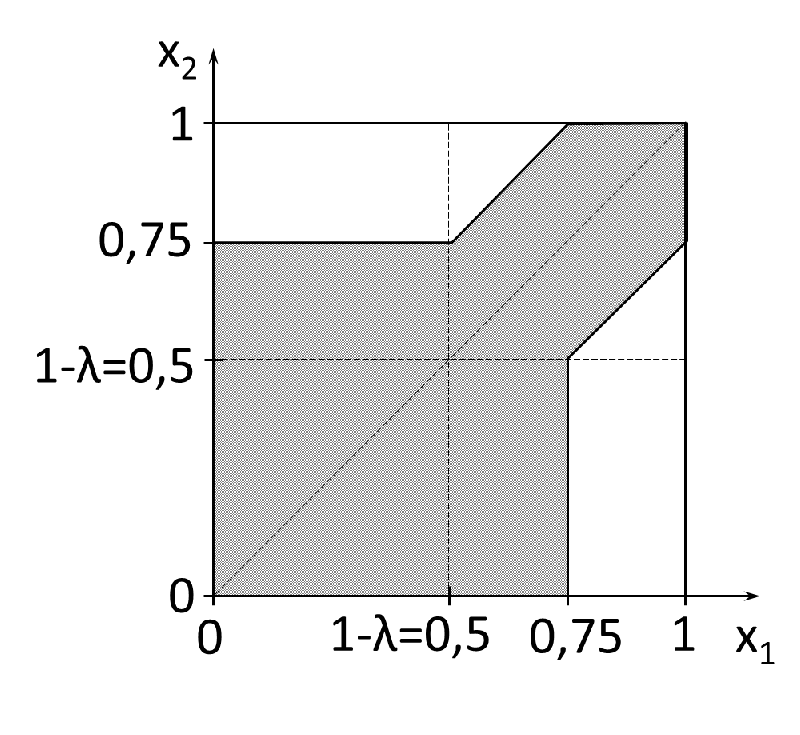
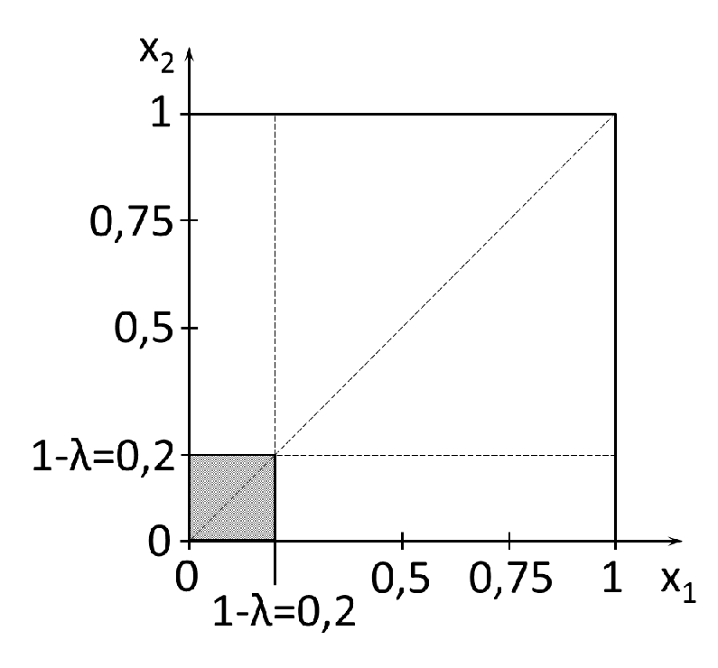
The relatively simple structure of the eigenspace in the previous example is influenced by the symmetry of the matrix $A$, which reduces the number of conditions that are to be considered. Now we show another two-dimensional example, in which all entries of the matrix have different values

There are five possible positions of the parameter $\lambda$ with respect to the diagonal entries $0.2$ and $0.4$, namely: $\lambda<0.2$, $\lambda=0.2$, $0.2<\lambda<0.4$, $\lambda=0.4$ and $\lambda>0.4$.

For $\lambda<0.4$, i.e. in the first three cases, the solution set is

In fact, it is the solution set for the second equation, whereas solution sets for the first equation in cases $\lambda<0.2$, $\lambda=0.2$ and $0.2<\lambda<0.4$ are: $\{x\colon x_{1}\leq 0.8\ \wedge\ x_{2}\leq 0.9\}$, $\{x\colon(x_{1}\leq 0.8\ \wedge\ x_{2}\leq 0.9)\ \vee\ (x_{1}>0.8\ \wedge\ -0.1+x_{2}\leq x_{1})\}$ and $\{x\colon(x_{1}\leq 1-\lambda\ \wedge\ x_{2}\leq 0.9)\ \vee\ (x_{1}>1-\lambda\ \wedge\ 0.1-\lambda+x_{2}=x_{1})\}$, respectively. All these sets contain the solution set (29), hence the intersection of the solutions for both equations is described by (29).

For $\lambda=0.4$ we obtain the solution sets for the first and the second equation

and their intersection is the solution set

For $\lambda>0.4$ we obtain the solution sets for the equations

Their intersection (the solution set) for $0.4<\lambda<0.7$ has the form

while for $\lambda\geq 0.7$ the solution set is simply

All described eigenspaces  (29), (31), (33) and (34) for $\lambda=0.35$, $\lambda=0.4$, $\lambda=0.55$ and $\lambda=0.85$ are displayed on Figure 3.

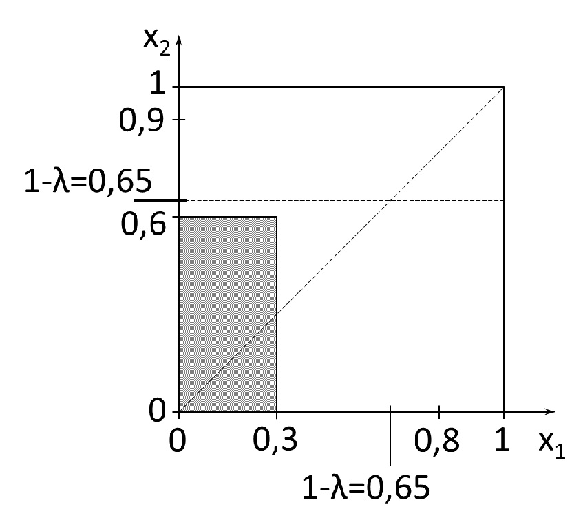
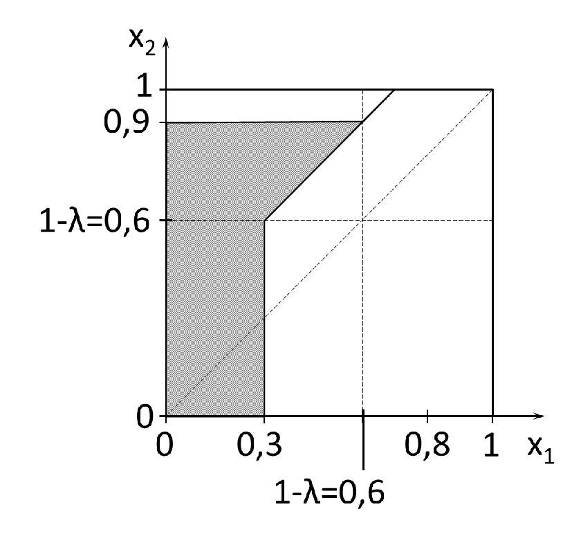
We now going to describe certain parts of the Łukasiewicz eigenspace, determined by the pattern of maxima on the r.h.s. of (16), whose generating sets (containing no more than $n+1$ points) can be written explicitly and computed in polynomial time.

References

- [1] M. Akian, R. Bapat, and S. Gaubert. Min-plus methods in eigenvalue perturbation theory and generalized Lidskiĭ-Višik-Ljusternik theorem. E-print arXiv:math/0402090v3, 2004-2006.
- [2] M. Akian, R. Bapat, and S. Gaubert. Max-plus algebras. In L. Hogben, editor, Handbook of Linear Algebra, volume 39 of Discrete Mathematics and Its Applications, chapter 25. Chapman and Hall/CRC, 2006.
- [3] X. Allamigeon. Static analysis of memory manipulations by abstract interpretation — Algorithmics of tropical polyhedra, and application to abstract interpretation. PhD thesis, École Polytechnique, Palaiseau, France, November 2009. http://www.lix.polytechnique.fr/Labo/Xavier.Allamigeon/papers/thesis.pdf.
- [4] F. L. Baccelli, G. Cohen, G. J. Olsder, and J. P. Quadrat. Synchronization and Linearity: an Algebra for Discrete Event Systems. Wiley, 1992.
- [5] P. Butkovič. Max-linear systems: theory and algorithms. Springer, 2010.
- [6] P. Butkovič and A. Aminu. Introduction to max-linear programming. IMA Journal of Management Mathematics, 2008.
- [7] P. Butkovič, H. Schneider, and S. Sergeev. Generators, extremals and bases of max cones. Linear Alg. Appl., 421:394–406, 2007.
- [8] P. Butkovič, H. Schneider, and S. Sergeev. Z-matrix equations in max-algebra, nonnegative linear algebra and other semirings. Linear and Multilinear Alg., 60(10):1191–1210, 2012. E-print arXiv:1110.4564.
- [9] Z.-Q. Cao, K.H. Kim, and F.W. Roush. Incline Algebra and its Applications. Chichester, 1984.
- [10] B.A. Carré. An algebra for network routing problems. J. of the Inst. of Maths. and Applics, 7, 1971.
- [11] K. Cechlárová. Powers of matrices over distributive lattices — a review. Fuzzy Sets and Systems, 138(3):627–641, 2003.
- [12] G. Cohen, D. Dubois, J.P. Quadrat, and M. Viot. A linear-system theoretic view of discrete-event processes and its use for performance evaluation in manufacturing, IEEE Transaction on Automatic Control, 30(3): 210–220, 1985.
- [13] G. Cohen, S. Gaubert, J. P. Quadrat, and I. Singer. Max-plus convex sets and functions. In G. Litvinov and V. Maslov, editors, Idempotent Mathematics and Mathematical Physics, volume 377 of Contemporary Mathematics, pages 105–129. AMS, Providence, 2005. E-print arXiv:math.FA/0308166.
- [14] R. A. Cuninghame-Green. Minimax Algebra, volume 166 of Lecture Notes in Economics and Mathematical Systems. Springer, Berlin, 1979.
- [15] R. A. Cuninghame-Green, K. Cechlárová. Residuation in fuzzy algebra and some applications. Fussy Sets and Systems, 71(2):227-239, 1995.
- [16] B. De Schutter. On the ultimate behavior of the sequence of consecutive powers of a matrix in the max-plus algebra. Linear Alg. Appl., 307:103–117, 2000.
- [17] M. Develin and B. Sturmfels. Tropical convexity. Documenta Math., 9:1–27, 2004. E-print arXiv:math.MG/0308254.
- [18] A. Di Nola and B. Gerla. Algebras of łukasiewicz’s logic and their semiring reducts. In G.L. Litvinov and V.P. Maslov, editors, Idempotent mathematics and mathematical physics, pages 131–144. 2005.
- [19] A. Di Nola, A. Lettieri, I. Perfilieva, V. Novák. Algebraic analysis of fuzzy systems. Fuzzy Sets and Systems, 158(1):1-22, 2007.
- [20] A. Di Nola and C. Russo. Łukasiewicz transform and its application to compression and reconstruction of digital images. Information Sci., 177:1481–1498, 2007.
- [21] A. Di Nola and C. Russo. Semiring and semimodule issues in mv-algebras. Communications in Algebra, 41:1017–1048, 2013.
- [22] M. Gavalec. Linear matrix period in max-plus algebra. Linear Alg. Appl., 307:167–182, 2000.
- [23] M. Gavalec. Periodicity in Extremal Algebras. Gaudeamus, Hradec Králové, 2004.
- [24] S. Gaubert and R. D. Katz. The Minkowski theorem for max-plus convex sets. Linear Alg. Appl., 421(2-3):356–369, 2007. E-print arXiv:math.GM/0605078.
- [25] S. Gaubert, R.D. Katz, and S. Sergeev. Tropical linear-fractional programming and parametric mean-payoff games. J. of Symbolic Computation, 47(12):1447–1478, 2012. E-print arXiv:1101.3431.
- [26] M. Gondran and M. Minoux. Graphs, Dioids and Semirings: New Applications and Algorithms. Springer, 2008.
- [27] M. Gondran and M. Minoux. Dioïds and Semirings: Links to fuzzy sets and other applications. Fuzzy Sets and Systems, 158:1273–1294, 2008.
- [28] S.-C. Han and H.-X. Li. Invertible incline matrices and Cramer’s rule over inclines. Linear Alg. Appl., 389:121–138, 2004.
- [29] M. Hartmann and C. Arguelles. Transience bounds for long walks. Mathematics of Operations Research, 24(2):414–439, 1999.
- [30] B. Heidergott, G.-J. Olsder, and J. van der Woude. Max-plus at Work. Princeton Univ. Press, 2005.
- [31] E.P. Klement, R. Mesiar, and E. Pap. Triangular Norms. Kluwer Academic Publ., Dordrecht, 2000.
- [32] N. K. Krivulin. On solution of generalized linear vector equations in idempotent algebra. Vestnik St.-Petersburg Univ. Math., 39:16–26, 2006.
- [33] N. K. Krivulin. Methods opf idempotent algebra in the problems of modeling and analysis of complex systems. St.-Petersburg Univ. Publ., 2009. in Russian.
- [34] G. L. Litvinov and V. P. Maslov. The correspondence principle for idempotent calculus and some computer applications. In J. Gunawardena, editor, Idempotency, pages 420–443. Cambridge Univ. Press, 1998. E-print arXiv:math/0101021.
- [35] M. Molnárová. Generalized matrix period in max-plus algebra. Linear Alg. Appl., 404:345–366, 2005.
- [36] I. Rashid, M. Gavalec, and S. Sergeev. Eigenspace of a three-dimensional max-Łukasiewicz fuzzy matrix. Kybernetika, 48(2):309–328, 2012.
- [37] S. Sergeev. Max algebraic powers of irreducible matrices in the periodic regime: An application of cyclic classes. Linear Alg. Appl., 431(6):1325–1339, 2009.
- [38] S. Sergeev. Max-algebraic attraction cones of nonnegative irreducible matrices. Linear Alg. Appl., 435(7):1736–1757, 2011.
- [39] S. Sergeev and H. Schneider. CSR expansions of matrix powers in max algebra. Trans. Amer. Math. Soc., 364:5969–5994, 2012. E-print arXiv:0912.2534.
- [40] Y.-J. Tan. On generalized fuzzy matrices with periods. Fuzzy Sets and Systems, 172(1):87–103, 2011.