Dynamic stabilization of the magnetic field surrounding the neutron electric dipole moment spectrometer at the Paul Scherrer Institute
Abstract
The Surrounding Field Compensation (SFC) system described in this work is installed around the four-layer Mu-metal magnetic shield of the neutron electric dipole moment spectrometer located at the Paul Scherrer Institute. The SFC system reduces the DC component of the external magnetic field by a factor of about 20. Within a control volume of approximately 2.5 m 2.5 m 3 m disturbances of the magnetic field are attenuated by factors of 5 to 50 at a bandwidth from Hz up to 0.5 Hz, which corresponds to integration times longer than several hundreds of seconds and represent the important timescale for the nEDM measurement. These shielding factors apply to random environmental noise from arbitrary sources. This is achieved via a proportional-integral feedback stabilization system that includes a regularized pseudoinverse matrix of proportionality factors which correlates magnetic field changes at all sensor positions to current changes in the SFC coils.
Keywords:
Magnetic field stabilization; magnetic field compensation; magnetic shielding; feedback stabilization; electric dipole momentpacs
07.55.Nk, 14.20.Dh, 13.40.Em, 41.20.GzI Introduction
In this work we describe the setup and performance of a stabilization system which monitors the environmental magnetic field and compensates for magnetic disturbances at several points around the respective control volume of roughly 10 m3 in size. This surrounding field compensation (SFC) system is an important part of the neutron electric dipole moment (nEDM) experiment [1, 2], located at the ultracold neutron (UCN) source [3, 4] of the Paul Scherrer Institute (PSI) in Villigen, Switzerland.
Ultracold neutrons have very low energies, below about 300 neV, and thus can be trapped in bottles and observed for times comparable to the lifetime of the free neutron. This fact makes them an excellent tool to search for a possible electric dipole moment of the neutron [5, 6, 1], which is considered to be one of the most important experiments in particle physics (see e.g. [7, 8, 9]) and will contribute to answering the fundamental questions on the origin of the matter-antimatter asymmetry observed in our universe. An introduction to UCN and the nEDM can be found in [10].
The nEDM experiment at PSI applies the Ramsey method of separated oscillatory fields [11] to spin-polarized UCN confined in a precession chamber located in the center of a vacuum tank inside a four layer Mu-metal magnetic shield. The sensitivity of the experiment depends on the stability of the internal magnetic field and field gradients inside the UCN storage chamber. Thus, of paramount importance for the measurement sensitivity are (i) a four-layer cylindrical magnetic shield made of Mu-metal (a high permeability NiFe-alloy) around the vacuum tank, and (ii) very high – tens of femtotesla – precision magnetometers in and around the UCN storage chamber to monitor the internal magnetic field changes. The stability and homogeneity of the magnetic field inside the shield depends to a large extent on the magnetization state of the Mu-metal. In order to maintain a stable magnetization, the surrounding magnetic field must be as stable as possible for magnetic field changes with frequencies below a few Hz. To fullfill this task the SFC system was set up around the Mu-metal shield. It provides a static compensation of the Earth’s magnetic field and additionally a dynamic compensation for the environmental magnetic field changes.
Our distinctive approach to the SFC system, described in detail in [12], uses a regularized pseudoinverse matrix of proportionality factors in the feedback algorithm and thereby avoids introducing noise in orthogonal directions (as e.g. in [13]). This allows us to stabilize the magnetic field simultaneously at many positions within the control volume. Our approach builds on previous experimental efforts at PSI [14] which used a simple dynamic magnetic field stabilization system. An overview of other magnetic field compensation systems published before the year 2005 can be found in [14].
While active surrounding magnetic field compensation is a necessity for high-sensitivity nEDM searches, it is also used in other particle physics experiments in order to achieve isotropic detector performance [15], in bio-magnetism [16, 17] and in medical research [18, 19] to improve signal and image quality.
II System characteristics
II.1 Overview


The six rectangular coils of the SFC, labeled the (X), (Y), and (Z)-coils, consist of copper wires with 6 mm2 cross section, mounted on aluminum frames, which are designed out of electrically isolated and ungrounded bars. They approximate a Helmholtz configuration as shown in Figs. 1 and 2. Table 1 summarizes important properties of the coils.
The origin of the experiment coordinate system is set at the center of the magnetic shield, which coincides with the center of the vacuum tank. Each coil pair is centered at this origin as well as possible, given physical constraints such as the presence of concrete blocks that are part of the biological shielding of the UCN source. The maximum offset from the center along any of the axes is less than 0.2 m.
The coils are driven by unipolar power supplies from FuG, type NTN350-35 and NTN700-35. These can provide 350 W and 700 W at a maximum voltage of 35 V. We have These power supplies are specified to a relative accuracy of 0.2 by the manufacturer. verified that the current can be controlled with 16-bit resolution. Usually the power supplies are operated at 70 % to 90 % of maximum current. Software-controlled solid state relays were added to the system to allow change of coil polarity. This was necessary because the superconducting test facilities SULTAN [20, 21] and EDIPO [22], at an approximate distance of 30 m from our setup, can cause a polarity change of the magnetic field in the horizontal plane at our experimental site during magnet ramping.
| Coil | X | X | Y | Y | Z | Z |
| Long side (m) | 7.9 | 7.9 | 8.2 | 8.4 | 8.0 | 8.0 |
| Short side (m) | 6.1 | 6.1 | 6.0 | 5.9 | 5.8 | 5.8 |
| Pair separation (m) | 4.2 | 5.1 | 4.2 | |||
| Windings | 18 | 18 | 9 | 9 | 12 | 12 |
| Resistance () | 2.0 | 2.0 | 1.0 | 1.0 | 1.3 | 1.3 |
| Inductance (mH) | 8 | 8 | 2 | 2 | 4 | 4 |
| Static current (A) | 8.7 | 8.7 | 7.3 | 7.3 | 14.0 | 14.0 |
The surrounding magnetic field is monitored with ten three-axis fluxgate magnetometers from Bartington, type Mag-03 MCL70 or MCTP70, mounted at the corners of the aluminum support structure of the Mu-metal shield, as shown in Fig. 1. The nomenclature of the sensors follows the pattern of fluxgate numbers FG 0-9 and their three orthogonal sensors in experiment coordinates: . Due to a sensor failure, fluxgate 4 (FG 4) was removed from the system. However, the entire system and signal treatment was developed to accommodate up to 30 sensors.
The sensor signals are sampled with two 16-bit multiplexing analog-to-digital converters (ADC) at a rate of 15.45 kHz per sensor. Before sampling, the signals are filtered by a passive low-pass filter with 43 Hz bandwidth which was chosen to suppress aliasing at the least significant bit level. The high sampling frequency, in combination with analog and digital filters, provides a high amplitude resolution of the sensor signal.
The same filters also ensure that the feedback system operates at frequencies significantly lower than the smallest magnetic resonance frequency in our system which is 8 Hz from a 199Hg magnetometer [1, 2]. Under these conditions the data acquisition (DAQ) system has an internal noise floor of 10 pT/, which corresponds approximately to the intrinsic sensor noise.
The SFC control software has two operation modes: (i) static, where the currents in the coils are constant and compensate the DC component of the ambient field; the stability of the current output was measured to be at the 10-5 level with an ohmic resistance as load; (ii) dynamic, where a digital feedback loop monitors the magnetic field and controls the currents at an iteration rate of 6 Hz, which is limited by the slow inherent settling time of the coil power supplies.
All relevant system properties are averaged if necessary and written to file at a rate of 1 Hz.
II.2 Magnetic field conditions for the nEDM measurement
Inside the Mu-metal shield of the nEDM experiment a cosine-theta coil wound around the cylindrical vacuum tank generates a vertical magnetic holding field of 1 T necessary for the Ramsey method. Up to 33 trim coils can be used to homogenize the field to a level better than 10-3. However, the holding field is superimposed by the remanent magnetic field of the Mu-metal shield. In order to demagnetize the shield, a so-called idealization procedure [23, 24] is applied. This procedure is analogous to a standard demagnetization but is done within a non-zero external and/or internal field and yields a reproducible remanent field of less than 1 nT inside the vacuum tank measured over the region of interest, in the case when the vertical holding field is turned off. For this reason the shield is idealized at least once a day, usually after a ramp of SULTAN or EDIPO. Keeping the surrounding magnetic field stable reduces the need for more frequent idealizations which would compete with nEDM measurement time. External perturbations can not only influence the magnitude of the holding field, but also locally destabilize the magnetization state of the Mu-metal shield, which may then lead to time-delayed changes of the Mu-metal magnetization. This effect combined with the high shielding factor of the Mu-metal causes that often no direct correlation between external – measured by fluxgates – and internal – measured by atomic magnetometers – magnetic field noise is observable. Thus, the control of the external magnetic field changes is done with the fluxgate sensors outside the magnetic shield, while the internal atomic magnetometers [25] are used to monitor the stability of the internal field.
II.3 Magnetic field characteristics at the nEDM site
The environmental surrounding magnetic field components in the experiment coordinate system are given by
| (1) |
at the coordinate system origin, measured before the experiment and the Mu-metal shield were installed, and with SULTAN and EDIPO turned off. The magnitude of this field is dominated by the Earth’s magnetic field. Additional static magnetic field contributions originate from the typical environment at large research facilities, e.g. radiation shielding made of iron and concrete, steel columns of building walls, etc. Gradients in the surrounding magnetic field and the distortion of the flux density due to the Mu-metal cause absolute magnetic field values measured at single fluxgate positions to range up to to 85 T.
Field perturbations during day-time occur rather frequently on a level of a few hundreds of nT. Figs. 3 shows a 1000 s long snapshot of the field measured with a fluxgate sensor a) or a Cs magnetometer b). Inside the Mu-metal shield the variations are observed with highly sensitive cesium magnetometers [25] operated inside in the 1 T magnetic holding field. All ten installed Cs magnetometers show a similar behavior and observe a strongly reduced amplitude. This confirms the passive shielding factor of our Mu-metal shield of order 104.
In order to demonstrate already here the power of our stabilization setup, we plot for comparison a similar situation with the field compensation working in dynamic mode (see Sec.III). Figs. 3c) and d) reflect the situation for a standard day-time data taking period. c) displays the measured field and the one calculated to be the original uncompensated field (see Eq.13). The suppression of the disturbances is obvious. In d) the corresponding measurement with a Cs magnetometer demonstrates that only one large field spike is not compensated sufficiently and observed inside the shield.

a) The measured uncompensated field shows up to 300 nT large variations; b) the Cs reading with smaller variations at the same time, reflecting the shielding of the Mu-metal shield. c) SFC in dynamic mode: the measured compensated field (lower red curve) and the uncompensated field (upper black curve); d) the corresponding Cs reading showing that all field variations were smaller than the magnetometer noise. Only one large field spike of more than 250 nT – 700 nT in the uncompensated field – at T=2530 s is also observed inside the shield.
The largest disturbance at the nEDM site occurs during regular field ramps of the neighboring SULTAN facility, a situation where nEDM measurements are stopped. Fig. 4a) shows the observed 7.7 T field change caused by a 2.5 T ramp at the position of sensor 5x without dynamic field compensation. At the same time the Cs magnetometer inside the Mu-metal shield observes a field change of about 180 pT (Fig. 4b). The measured field change caused by a 5 T ramp with dynamic field compensation on is plotted in Figs. 4c) and d). Outside the shield this disturbance is reduced by a shielding factor of about 20. The ten available Cs magnetometers inside the shield show corresponding shielding factors between 11 and 24. Clearly we can state, that the suppression of disturbances by dynamic SFC and passive magnetic shield multiply.

The bandwidth of magnetic noise or perturbations which the compensation system is able to attenuate extends from 0.5 Hz down to Hz. This corresponds to time ranges of seconds to hours, which are the important time scales for the nEDM experiment. Single nEDM measurements last from about 100 s up to 300 s, and measurement sequences for one parameter set take several hours. Therefore, the magnetic field should be stable over such time scales. Magnetic noise within this bandwidth is created at the site by neighboring experiments, passing vehicles, cranes, and other moving objects.
The stability of the magnetic field can be quantified via the Allan deviation [26] which is a function of integration time :
| (2) |
where =/ with being the total time of the measurement and the average magnetic field of the subsample over time . The Allan deviation of time is thus a measure of the average stability of the magnetic field at integration time . As shown in Fig. 5, typical stability levels without dynamic stabilization range from 10 nT to 100 nT during daytime – without ramps – and below 1 nT at nighttime and on weekends.

II.4 Performance limitations
The performance of the SFC is not only limited by its response bandwidth, but also by the number of adjustable coil currents, resulting in six degrees of freedom. A system of six coils generates fields dominated by constant terms and some first order gradients. In general, a first order gradient perturbation – consisting of both constant and linear terms – contains eight independent parameters: three homogeneous field components and five independent parameters of the gradient tensor. Thus, the compensation system is most effective at attenuating uniform magnetic field changes, e.g. from magnetic field sources located far away. Perturbations with their origin very close to, or even inside the SFC volume can only be partially attenuated. Therefore, care must be taken to keep sources of magnetic noise away from the sensitive volume of the experiment.
III Feedback algorithm for dynamic compensation
III.1 Structure of the feedback algorithm
| Index | Quantity | Values |
|---|---|---|
| Feedback iteration | ||
| Coil | ||
| Sensor | ||
| Feedback sensor | Subset of |
In this work the currents and magnetic field values are summarized in arrays of size 6 and 27, corresponding to the respective coils (index ) and field sensors (index ). An array, as well as each array element, can have a superscript index referring to an iteration of the feedback loop, e.g. is the current in coil in iteration . This indexing convention is summarized in Tab. 2.

A flow chart of the main structure of the SFC control algorithm is given in Fig. 6. In static mode, constant currents, , are applied to all coils. During standard magnetic field conditions (SULTAN and EDIPO not in operation), the control system applies the currents given in Tab. 1. They partly compensate for the DC component of the environmental field and yield low absolute magnetic field values (Sec. V.1). The target-value of the magnetic field is not predefined within the feedback algorithm. Instead, when switching from static to dynamic mode, the target-value is set to the actual read-value of the magnetic field at the instant of switching to avoid sudden field changes. Once magnetic field perturbations occur, the read-value will change and deviate from the target-value. Within each iteration of the feedback loop, the difference between and should be reduced by determining an appropriate array of six new current set-values .
The distinctive feature of the algorithm is a matrix of proportionality factors which correlate magnetic field changes at all sensor positions to current changes in the SFC coils. This matrix (Sec. III.2) is used to calculate the new current set-values in each iteration of the feedback loop (step D). Before the matrix can be included as a constant into the feedback loop, it has to be inverted and regularized once (see Sec. III.3). Approaches containing a regularized or truncated pseudoinverse are also known from bio-magnetometry [27, 28], where the sources of magnetic signals (e.g. from magnetically targeted drugs) are derived from measured magnetic fields. Another application is the localization of ferromagnetic objects buried in the ground [29, 30].
III.2 Calculating a new current set-value
In an earlier version of the feedback algorithm each coil current was controlled individually to stabilize one sensor reading, i.e. six sensors were used as feedback sensors. This method had the drawback that the field was stabilized very well at the positions of the feedback sensors, but not anywhere else within the SFC volume. An example of such behavior is given in Fig. 12. Presently we employ a more advanced method which enables us to use more than six feedback sensors and, thus, transfers the stabilizing effect of dynamic compensation from certain single points to the requested control volume.
The matrix of proportionality factors

We checked that each fluxgate sensor has a linear response to current changes in each of the six SFC coils. These proportionality factors (with units of nT/A) are summarized in a matrix which is defined as:
| (3) |
In the SFC setup the matrix elements, i.e. the proportionality factors (hereafter used synonymously), vary by three orders of magnitude and reach values of up to a few 1000 nT/A. Their magnitudes depend on the orientation and specific position of the sensors, the distances to the SFC coils and the magnetic shield, and on irregularities of the Mu-metal, such as overlaps, feedthroughs, and welded joints. A color map of the absolute values of the matrix elements is shown in Fig. 7. A pattern is recognizable and each sensor has the largest response to the particular coil which corresponds best to its orientation and position. For example, the largest matrix element of sensor 0x is since it is aligned in the x-direction and mounted on the (X+)-side of the shield.
Including the proportionality matrix into a proportional-integral feedback algorithm
In order to reduce the difference between and in a feedback loop, a compensating magnetic field has to be generated by modifying the coil currents. This new current is calculated by inverting Eq. 3. Since is not a square matrix, we use the Moore-Penrose pseudoinverse [31, 32] hereafter named pseudoinverse or . Thus, when evaluating the change () to a new current set-value, all 27 available sensors can be taken into account:
| (4) |
where is the difference between the target-value and the read-value of sensor .
To improve the stabilizing effect of dynamic SFC, the number of feedback sensors should theoretically be as high as possible. However, using all available sensors as feedback sensors has the disadvantage that there are then no reference sensors left and no information about the magnetic field stability at non-stabilized points is available. To avoid this, and to investigate the influence of the number of feedback sensors on the achieved stabilization, we tested the process with a subset of size . Inserting Eq. 4 into a proportional-integral (PI) feedback algorithm yields the following formula for each current set-value at iteration :
| (5) |
where are the coil currents at the moment of switching into dynamic mode (Fig. 6, step A). The compensation can be tuned individually with the proportional and integral gains and for each coil . is given by
| (6) |
where is the pseudoinverse of a submatrix of which contains only the proportionality factors of the chosen sensors used for the feedback. The dimension of is thus .
III.3 Matrix inversion and regularization
The pseudoinverse of a matrix is calculated via the singular value decomposition [33]:
| (7) |
where and are unitary matrices and is a real diagonal matrix of the same dimensions as , which contains the singular values of .
Tests showed that applying the method described so far yields unsatisfactory results for our feedback system as the stability of the magnetic field decreased in the dynamic mode. This can be explained by the large differences in magnitude between the individual matrix elements , i.e. the matrix is ill-conditioned. As a consequence, sensors with smaller matrix elements have larger weights after matrix inversion. Noise on one of these sensors will then be overcompensated and lead to instabilities. Such effects are accompanied by large amplitudes in the current change during dynamic stabilization. In order to avoid such noise amplification, a regularization is applied to the inversion, in our case a Tikhonov regularization [34]. This method replaces the inverted singular values of the matrix in the following way:
| (8) |
where and is the regularization parameter with a range of .
The limit corresponds to the non-regularized pseudoinverse of the matrix . Setting to will result in , and, from Eq. 7, it will also result that . The regularization has the greatest effect when is of the order of , which corresponds to approximately in our case.
Determination of the regularization parameter

We simulated a simplified compensation model which includes the measured proportionality factors in order to choose an appropriate value of . A flow chart of the concept is shown in Fig. 8.
First (step A in Fig. 8), for the chosen number of feedback sensors magnetic field values are picked at random, from a normal distribution that is based on the noise spectrum observed at the apparatus in the bandwidth of interest, to form .
Next (step B), an array of simulated current set-values is calculated using Eq. 6:
| (9) |
varies not only as a function of , but also as a function of . Thus many different have to be compared in order to determine how much the response of our feedback can vary. Typical field change distributions observed in the real system are shown in Appendix E5 of Ref. [12].
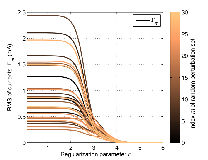
As a figure of merit, the root mean square (RMS) of the currents, , is defined as a function of :
| (10) |
In the following example we used 30 different sets of indexed with . The 30 resulting for the different are plotted in Fig. 9 with each indicated in a different color. With increasing regularization parameter, the magnitude of the currents in the SFC coils decreases. Lower compensation currents (not the DC part though) indicate smaller overcompensation, but if currents are too small the stabilizing effect will vanish; hence a compromise has to be found. The resulting magnetic field is a superposition of the perturbation and the field caused by . This field can be calculated with the original submatrix of the feedback sensors (step C). Thus as function of is given by:
| (11) |
In order to evaluate the effect of the simulated currents on the field perturbation, we compare the RMS of to the RMS of the resulting compensated field (step D),
| (12) |
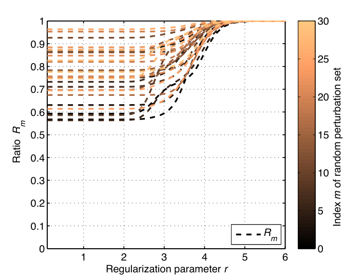
via the ratio .
If the perturbation was compensated completely, the resulting field, and the ratio would be zero. The dependence of for the same 30 values of on the regularization parameter is shown in Fig. 10. One can see that if the regularization parameter is too large, the compensation effect collapses completely as a consequence of the vanishing currents. This figure also shows that in this simulated case, perturbations can only be compensated for by a maximum of 45%, a behavior also observed in the real system.
In order to find the optimal value for , it is convenient to normalize and such that their minimum and maximum values lie between 0 and 1. The resulting quantities and are shown in Fig. 11. The regularization parameter is finally determined in the following way (step E): 1000 different random values of are generated.
For each random perturbation the values of corresponding to and to (as indicated in Fig. 11 by the horizontal solid grid-line) are stored. These 2000 values of are then averaged. In the model example shown here, the final result of the described procedure is . The regularized pseudoinverse resulting from is then fixed in the feedback algorithm.
A further fine tuning of the feedback behavior is possible via and . Using different amplitudes and widths for the normal distribution from which we extract , we have found that the qualitative behavior of and does not depend on the magnitude of the perturbation. The specific dependence on the regularization parameter is rather a property of the matrix itself, i.e. of the particular subset of chosen feedback sensors. Each time a different set of feedback sensors is used, is re-determined in the way described above and the resulting regularized pseudoinverse is inserted into the feedback algorithm.
In general, we can compare tuning to changing : in Fig. 11 one can see that close to the chosen value of the regularization parameter, the dependency of the current on can be approximated to be linear. In this way, the final fine tuning of the system can be achieved without recalculating a new regularized matrix. are finally chosen to achieve a fast system response and avoid overshooting. Further detailed information about gain tuning can be found in Ref. [12].
IV A method to quantify the SFC performance
IV.1 General comments on shielding factors
There exist many different approaches to quantifying the performance of an active stabilization system for magnetic fields, depending on each specific setup. Often shielding factors include the passive shielding provided by a high permeability magnetic shield, such as our Mu-metal shield, which is usually one order of magnitude per shielding layer at frequencies around 1 Hz and increasing for higher frequencies, as e.g. in [35]. It is also common to investigate the shielding performance with artificial noise sources such as dedicated coils [36]. Such tests have limited significance since the coils are often of the same geometry as the compensation coils and thus generate a similar field. Furthermore, the excitation coils are typically mounted with their axes parallel to one of the axes of the compensation setup. As a consequence, the shielding factors are only determined for one direction [14], neglecting the fact that one-dimensional corrections can increase the noise level in orthogonal directions. This is referred to as cross-axial interference in [36]. Realistic shielding factors for arbitrary environmental magnetic noise are usually much smaller. They are also more difficult to estimate, since random noise, as typically present in an accelerator facility such as ours, cannot be easily reproduced. The method presented here allows determining the shielding factors of all sensors in a single measurement and does not rely on comparing measurements with compensation “on” vs. “off”.
IV.2 Definition of the shielding factor
To investigate the impact of the SFC on the stability of the magnetic field, the measured field is interpreted as a superposition of the uncompensated field and the additional magnetic field created by the SFC coils at all sensor positions:
| (13) |
The field generated by the coils can be calculated via
| (14) |
and the magnetic field without the compensation effect can be extracted. The applied current values as measured by the coil power supplies are used. The Allan deviation (Eq. 2) is used as a measure of the magnetic field stability. Comparing of to that of the measured magnetic field reveals if the noise level is decreased by applying the SFC in dynamic mode. The ratio of both shows the factor by which the stability was improved at a given integration time for each specific measurement, independent of any reproducibility of the surrounding magnetic field properties. The active shielding factor for each sensor is thus defined as
| (15) |
regardless whether is a feedback sensor or not. therefore reflects the improvement under real environmental conditions.
The largest possible integration time for a time series of length is . For computational reasons we calculate the shielding factor only for s. Thus, each time series under consideration is truncated to . In this way the same portion of the time series is regarded for each . is omitted in the plots shown in Sec. V. The length of the measured time series was at least four times the largest given integration time.
A measurement with SFC in static mode, where the DC component of the environmental field is compensated, results in = 1.000000.00001 for all integration times and therefore confirms the validity of the shielding factor definition. This demonstrates that including the coil currents in the shielding factor calculation (Eq. 14) does not significantly affect the shielding factor values.
The statistical errors on the level of single magnetic field measurements have a negligible contribution to the shielding factor. The observed spread of shielding factors at various positions (plotted for several conditions in Sec. V) represents in our experience a measure for the uncertainty of the shielding factor.
V Performance of the SFC system
V.1 Reduction of the DC component of the magnetic field around the Mu-metal shield
The amplitudes of magnetic perturbations are usually much smaller than the absolute value of the surrounding magnetic field given in Eq. 1. Thus, for the static operation mode, a set of standardized currents was derived (Tab. 1) which decreases the absolute value of the surrounding magnetic field to at least below 10 T at all sensor positions but exceptions up to 15 T may occur at two sensor positions. These standard currents are also set during the demagnetization procedure of the shield. The average DC reduction factor is about 20 or larger.
V.2 Performance of the SFC with six independent fluxgate sensors
In a simple feedback mode, six sensors are used to control the six SFC coil currents as listed in Tab. 3 via six independent control loops.
| Coil | X | X | Y | Y | Z | Z |
|---|---|---|---|---|---|---|
| Feedback sensor | 5x | 1x | 5y | 1y | 5z | 1z |
| 0.95 | 0.92 | 0.98 | 0.94 | 0.45 | 0.50 | |
| 0.44 | 0.45 | 0.42 | 0.39 | 0.35 | 0.32 |
The fluxgate sensors FG 1(x,y,z) and FG 5(x,y,z) were located at positions and (full circles in Fig. 1). Each position is at the crossing point of the three coil planes. There, the smallest value for the response of fluxgate sensors orthogonal to the axis of a given coil was found. The signal was about 10 % of the sensor parallel to the coil axis. The stabilization worked well only at the positions of the feedback sensors. The stabilizing effect showed a huge discrepancy between the feedback sensors and all other sensors, as shown in Fig. 12. The shielding factor for the feedback sensors (dashed lines) reached values up to 103 and above for s, while other sensors showed low values from 2 to 4 or even indicated a decrease in stability in dynamic mode, e.g. , (Fig. 12, bottom). Such a decrease of stability was even more prominent in magnetically quiet times when very small perturbations at the positions of FG 1 or FG 5 were overcompensated and projected onto the entire control volume.

V.3 Comparison of the SFC performance with twelve feedback sensors with a non-regularized and a regularized matrix.


The shielding factors measured with twelve feedback sensors, using a non-regularized pseudoinverse of the matrix of proportionality factors are shown in Fig. 13. The feedback sensors were distributed over the entire control volume with an equal number of x-, y-, and z-sensors. The monitor sensors are depicted with solid lines. Gains were used for all . The measured shielding factors were spread over a wide range, and most of them were below one. Thus, the stability of the magnetic field was significantly decreased, caused by overcompensation of noise in sensor 0x, which showed a factor of four stability improvement. In order to mitigate this overcompensation, a regularization with was applied. The effect of the regularization on the matrix elements of the individual sensors is displayed in Fig. 14 as a color-map of the absolute values of the differences . Indeed, the matrix elements of sensor 0x are most affected by the regularization.
Dynamic feedback stabilization with the regularized matrix increased the shielding factors as shown in Fig. 15. and were used for all . The smaller spread of the shielding factor values indicates that the stabilization effect by dynamic SFC was more homogeneous at different sensor positions. The stability improved by factors of 4 to 30 at integration times greater than 10 s at almost all sensor positions. This demonstrates that using a regularized pseudoinverse matrix of proportionality factors is an effective way to take into account the entanglement of all sensors and coils and transfer the stabilization of the magnetic field at single feedback sensor positions to a larger volume.
V.4 SFC performance with 18 and 24 feedback sensors

We also investigated the influence of 18 and 24 feedback sensors on the SFC stabilization performance. Figure 16 shows the shielding factors achieved with 18 feedback sensors, , , and for all . For feedback three sensors of FG 1 and FG 5 and two sensors each of FG 2, FG 3, FG 4, FG 6, FG 7 and FG 9 were selected. The achieved shielding factors cover a range from 2 to 50 for s, comparable to the regularized case with 12 sensors.
Figure 17 shows the shielding factors achieved with 24 feedback sensors, , , and for all . Only sensors 6y, 5z, and 6z were not used for the feedback. The behavior is slightly different compared to the 18-sensor feedback. The shielding factors are quite low for s which is probably caused by picking up noise of higher multipole order which cannot be compensated by the present system. Opening and closing of shutters or valves in the nEDM experiment with operation times of a few seconds could be the source of this noise. For s the shielding factors increased and reach a similar level as for the 12- and 18-sensor feedback. The observed shielding factors agree with amplitude suppression of single-disturbance events, as e.g. shown in Fig.3.

V.5 SFC performance with large field changes caused by remote sources

The highest shielding factors observed so far were during the approximately hour-long magnetic field changes during ramping of the neighboring superconducting magnets SULTAN or EDIPO. These events cause a field change of up to 30 T at our experiment position in case of a full 12 T ramp. The two remote magnetic field sources differ in stray field magnitude, but have only small higher order multipoles at the position of our experiment. Therefore, the SFC system can compensate for these perturbations very well, as shown in Fig. 18. Fig. 4 shows the observed field values in a single sensor during a SULTAN ramp outside and inside the Mu-metal shield and also the achieved compensation with the SFC system. Nevertheless, the ramp can only be attenuated, the remaining field change, in spite of dynamic SFC, can be up to 2 T at single sensor positions outside the shield. A dedicated coil system which creates the particular compensation fields for SULTAN or EDIPO would be necessary in order to fully offset those ramps. However, with an idealization procedure as described in [23], the absolute value, as well as the three components of the magnetic field inside the Mu-metal shield, were reproduced to within a few hundreds of pT of the values before the ramp, as measured with scalar and vector magnetometers inside the Mu-metal shield. The observed shielding factors up to about 100 show the potential of the applied method for remote disturbances.
VI Conclusions and outlook
We have shown that the SFC reduces and stabilizes the magnetic field around and inside the Mu-metal shield of our apparatus. This is important for conducting the nEDM measurements, specifically in the time range from 100 s to 300 s.
When using a simple feedback algorithm without implementation of a matrix of proportionality factors, high shielding factors were achieved only at the locations of the chosen feedback sensors. The obtained shielding factors in the control volume ranged from 2 to 5. At magnetically quiet times, such a simple feedback type even decreased the field stability slightly.
The shielding factors were increased to values of 3 to 50 by including a regularized pseudoinverse matrix of proportionality factors. No significant difference was observed in the quality of the magnitude of the shielding factors at stabilized and non-stabilized sensor positions. Furthermore, comparable results were achieved at magnetically noisy periods and at quiet times.
We have shown that in our setup the shielding factors do not improve when the number of feedback sensors is increased from 12 to 18 or to 24. On the contrary, the shielding factors for short integration times (s) decrease with increasing number of feedback sensors, which may pick up very localized higher-order multipole magnetic noise.
In the case of remote magnetic disturbances containing no, or only small higher-order, multipole contributions, shielding factors of up to 100 were achieved.
The performance of the SFC system could be extended to compensate for higher multipole field perturbations by increasing the number of coils in the system. R&D for systems with a larger number of coils and field sensors are being pursued, together with further refinement of the SFC feedback model.
VII Acknowledgements
The Paul Scherrer Institute and ETH Zürich gratefully acknowledge the support of the Swiss National Science Foundation under Grant Nos. 200021_126562, 200020_144473, 200021_138211, 200020_149211 and CRSII2_144257. University of Fribourg acknowledges financial support by Grant 200020_140421 of the Swiss National Science Foundation. KU Leuven acknowledges the support of the Fund for Scientific Research Flanders (FWO) and Project GOA/2010/10 of the KU Leuven. LPC Caen and LPSC Grenoble acknowledge Grant No. ANR-09-BLAN-0046. Jagellonian University Cracow acknowledges support by the Foundation for Polish Science - MPD program, co-financed by the European Union within the European Regional Development Fund, and by the National Science Centre, Poland, under Grant No. 2012/04/M/ST2/00556. The contribution of TU München in the beginning of the project is acknowledged.
References
- [1] C. Baker, G. Ban, K. Bodek, M. Burghoff, Z. Chowdhuri, M. Daum, M. Fertl, B. Franke, P. Geltenbort, K. Green, M. van der Grinten, E. Gutsmiedl, P. Harris, R. Henneck, P. Iaydjiev, S. Ivanov, N. Khomutov, M. Kasprzak, K. Kirch, S. Kistryn, S. Knappe-Gr¨uneberg, A. Knecht, P. Knowles, A. Kozela, B. Lauss, T. Lefort, Y. Lemiere, O. Naviliat-Cuncic, J. Pendlebury, E. Pierre, F. Piegsa, G. Pignol, G. Quémener, S. Roccia, P. Schmidt-Wellenburg, D. Shiers, K. Smith, A. Schnabel, L. Trahms, A. Weis, J. Zejma, J. Zenner, and G. Zsigmond, Physics Procedia 17, 159 (2011).
- [2] C. Baker, Y. Chibane, M. Chouder, P. Geltenbort, K. Green, P. Harris, B. Heckel, P. Iaydjiev, S. Ivanov, I. Kilvington, S. Lamoreaux, D. May, J. Pendlebury, J. Richardson, D. Shiers, K. Smith, and M. van der Grinten, Nuclear Instruments and Methods in Physics Research Section A 736, 184 (2014).
- [3] B. Lauss, Hyperfine Interactions 211, 21 (2012).
- [4] B. Lauss, Physics Procedia 51, 98 (2014).
- [5] C. A. Baker, D. D. Doyle, P. Geltenbort, K. Green, M. G. D. van der Grinten, P. G. Harris, P. Iaydjiev, S. N. Ivanov, D. J. R. May, J. M. Pendlebury, J. D. Richardson, D. Shiers, and K. F. Smith, Phys. Rev. Lett. 97, 131801 (2006).
- [6] A. Serebrov, E. Kolomenskiy, A. Pirozhkov, I. Krasnoschekova, A. Vassiljev, A. Polushkin, M. Lasakov, A. Fomin, I. Shoka, V. Solovey, O. Zherebtsov, P. Geltenbort, S. Ivanov, O. Zimmer, E. Alexandrov, S. Dmitriev, and N. Dovator, JETP Letters 99, 4 (2014).
- [7] R. Lamoreaux, S. K. Golub, Lepton Dipole Moments. Series: Advanced Series on Directions in High Energy Physics, ISBN: 978-981-4271-83-7. WORLD SCIENTIFIC, Edited by B Lee Roberts and William J Marciano, vol. 20, pp. 583-634 .
- [8] M. Raidal, A. Schaaf, I. Bigi, M. Mangano, Y. Semertzidis, S. Abel, S. Albino, S. Antusch, E. Arganda, B. Bajc, S. Banerjee, C. Biggio, M. Blanke, W. Bonivento, G. Branco, D. Bryman, A. Buras, L. Calibbi, A. Ceccucci, P. Chankowski, S. Davidson, A. Deandrea, D. DeMille, F. Deppisch, M. Diaz, B. Duling, M. Felcini, W. Fetscher, F. Forti, D. Ghosh, M. Giffels, M. Giorgi, G. Giudice, E. Goudzovskij, T. Han, P. Harris, M. Herrero, J. Hisano, R. Holt, K. Huitu, A. Ibarra, O. Igonkina, A. Ilakovac, J. Imazato, G. Isidori, F. Joaquim, M. Kadastik, Y. Kajiyama, S. King, K. Kirch, M. Kozlov, M. Krawczyk, T. Kress, O. Lebedev, A. Lusiani, E. Ma, G. Marchiori, A. Masiero, I. Masina, G. Moreau, T. Mori, M. Muntel, N. Neri, F. Nesti, C. Onderwater, P. Paradisi, S. Petcov, M. Picariello, V. Porretti, A. Poschenrieder, M. Pospelov, L. Rebane, M. Rebelo, A. Ritz, L. Roberts, A. Romanino, J. Roney, A. Rossi, R. Rückl, G. Senjanovic, N. Serra, T. Shindou, Y. Takanishi, C. Tarantino, A. Teixeira, E. Torrente-Lujan, K. Turzynski, T. Underwood, S. Vempati, and O. Vives, The European Physical Journal C 57, 13 (2008).
- [9] CERN Council, “European strategy for particle physics - update 2013,” (2013), s/106.
- [10] R. Golub, D. Richardson, S.K. Lamoreaux, Ultra-Cold Neutrons, Gol (Adam Hilger - Bristol, New York, Philadelphia, 1991).
- [11] N. F. Ramsey, Physical Review 76, 996 (1949).
- [12] B. Franke, Investigations of the Internal and External Magnetic Fields of the Neutron Electric Dipole Moment Experiment at the Paul Scherrer Institute, Phd thesis no. 21562, ETH Zürich (2014).
- [13] J. Belfi, G. Bevilacqua, V. Biancalana, R. Cecchi, Y. Dancheva, and L. Moi, Review of Scientific Instruments 81, 065103 (2010), 10.1063/1.3441980.
- [14] T. Brys, S. Czekaj, M. Daum, P. Fierlinger, D. George, R. Henneck, M. Kasprzak, K. Kirch, M. Kuzniak, G. Kuehne, A. Pichlmaier, A. Siodmok, A. Szelc, L. Tanner, C. Assmann, S. Bechstein, D. Drung, T. Schurig, C. Ciofi, and B. Neri, Nuclear Instruments and Methods in Physics Research, Section A 554, 527 (2005).
- [15] M. Bodmer, F. Giuliani, M. Gold, A. Christou, and M. Batygov, Nuclear Instruments and Methods in Physics Research, Section A 697, 99 (2013).
- [16] O. Baltag, D. Costandache, M. Rau, A. Iftemie, and I. Rau, Advances in Electrical and Computer Engineering 10, 135 (2010).
- [17] O. Baltag, D. Costandache, and M. C. Rau, Journal of Basic and Applied Physics 1, 9 (2012).
- [18] Y. Nakashima and I. Sasada, Journal of Applied Physics 105, 07A336 (2009).
- [19] H. Dong, L. Qiu, W. Shi, B. Chang, Y. Qiu, L. Xu, C. Liu, Y. Zhang, H.-J. Krause, A. Offenhaeusser, and X. Xie, Applied Physics Letters 102, 102602 (2013).
- [20] P. Bruzzone, A. Anghel, A. Fuchs, G. Pasztor, B. Stepanov, M. Vogel, and G. Vecsey, IEEE Transactions on Applied Superconductivity 12, 520 (2002).
- [21] B. Stepanov, P. Bruzzone, K. Sedlak, and G. Croari, Fusion Engineering and Design 88, 282 (2013).
- [22] A. Portone, J. Amend, W. Baker, P. Bruzzone, F. Cau, G. Croari, E. Fernandez-Cano, S. March, E. Salpietro, H. Scheller, B. Stepanov, E. Theisen, M. Vogel, and R. Wesche, IEEE Transactions on Applied Superconductivity 22, 4202905 (2012).
- [23] F. Thiel, IEEE Transactions on magnetics 45, 12, 5307 (2009).
- [24] S. Knappe-Grueneberg, A. Schnabel, G. Wuebbeler, and M. Burghoff, Journal of Applied Physics 103, 07E925 (2008).
- [25] P. Knowles, G. Bison, N. Castagna, A. Hofer, A. Mtchedlishvili, A. Pazgalev, and A. Weis, Particle Physics with Slow Neutrons, Nuclear Instruments and Methods in Physics Research Section A: Accelerators, Spectrometers, Detectors and Associated Equipment 611, 306 (1).
- [26] J. A. Barnes, A. R. Chi, L. S. Cutler, D. J. Healey, D. B. Leeson, T. E. McGunigal, J. A. Mullen, W. L. Smith, R. L. Sydnor, R. F. C. Vessot, and G. M. R. Winkler, IEEE Transactions on Instrumentation and Measurement IM-20, 105 (1971).
- [27] D. Baumgarten, M. Liehr, F. Wiekhorst, U. Steinhoff, P. Münster, P. Miethe, L. Trahms, and J. Haueisen, Medical and Biological Engineering and Computing 46, 1177 (2008).
- [28] D. Baumgarten and J. Haueisen, IEEE Transactions on Magnetics 46, 3496 (2010).
- [29] R. Eichardt, D. Baumgarten, L. Di Rienzo, S. Linzen, V. Schultze, and J. Haueisen, COMPEL - The International Journal for Computation and Mathematics in Electrical and Electronic Engineering 28, 1327 (2009).
- [30] R. Eichardt and J. Haueisen, IEEE Transactions on Magnetics 46, 3449 (2010).
- [31] E. Moore, Bulletin of the American Mathematical Society 26, 394 (1920).
- [32] R. Penrose, Mathematical Proceedings of the Cambridge Philosophical Society 51, 406 (1955).
- [33] G. Golub and W. Kahan, Journal of the Society for Industrial and Applied Mathematics Series B Numerical Analysis 2, 205 (1965).
- [34] H. Engl, M. Hanke, and A. Neubauer, Regularization of Inverse Problems (Kluwer Academic Publishers, Dordrecht, Netherlands, 2000).
- [35] H. J. M. ter Brake, R. Huonker, and H. Rogalla, Measurement Science and Technology 4, 1370 (1993).
- [36] K. Kobayashi, A. Kon, M. Yoshizawa, and Y. Uchikawa, IEEE Transactions on Magnetics 48, 4554 (2012).