The Smart Kinetic Self-Avoiding Walk and
Schramm Loewner Evolution
Abstract
The smart kinetic self-avoiding walk (SKSAW) is a random walk which never intersects itself and grows forever when run in the full-plane. At each time step the walk chooses the next step uniformly from among the allowable nearest neighbors of the current endpoint of the walk. In the full-plane a nearest neighbor is allowable if it has not been visited before and there is a path from the nearest neighbor to infinity through sites that have not been visited before. It is well known that on the hexagonal lattice the SKSAW in a bounded domain between two boundary points is equivalent to an interface in critical percolation, and hence its scaling limit is the chordal Schramm-Loewner evolution with (SLE6). Like SLE there are variants of the SKSAW depending on the domain and the initial and terminal points. On the hexagonal lattice these variants have been shown to converge to the corresponding version of SLE6. It is believed that the scaling limit of all these variants on any regular lattice is the corresponding version of SLE6. We test this conjecture for the square lattice by simulating the SKSAW in the full-plane and find excellent agreement with the predictions of full-plane SLE6.
1 Introduction
There are a variety of models that produce random walks that are simple, i.e., walks that do not have any self-intersections. In the self-avoiding walk (SAW) model, all simple walks with the same number of steps are given the same probability [16]. The scaling limit of this model is conjectured to be SLE8/3 (Schramm-Loewner evolution with ) [13], and there is numerical evidence to support this conjecture [8, 9]. Loop-erased random walks (LERW) are generated by erasing the loops in an ordinary random walk in chronological order. The scaling limit of this model has been proved to be SLE2 [14].
In this paper we study another model of simple random walks in the plane that was introduced in the physics literature in the mid 1980’s under a couple of names. We will refer to it as the smart kinetic self-avoiding walk (SKSAW) for reasons we will explain later. The model can be defined on any lattice in any number of dimensions, but our study will only be concerned with two dimensions. We are particularly interested in the relationship of the scaling limit of this model with SLE6.

There are several versions of the SKSAW corresponding to different choices of the region in which the walk takes place and the choice of initial and terminal points. We first define one that we will call the “full-plane” SKSAW. We start the walk at the origin, i.e., . For the first step we choose one of the nearest neighbors of the origin with equal probability. Now suppose the steps have been chosen for . We say that a site is occupied if the walk has visited before, i.e., for some . We say that is a trapping site (with respect to ) if there does not exist a nearest neighbor path from to though unoccupied sites. Figure 1 illustrates these definitions. Now consider the nearest neighbors of that are not occupied and are not trapping sites. We assign them equal probability and choose one at random to be . A simple induction argument shows there is always at least one such nearest neighbor. (Because was not a trapping site when it was chosen, it is connected to .) This process will run forever and generate a self-avoiding walk in the plane from to . So we will refer to it as the full-plane SKSAW from to .
The next version we consider is also defined in the full-plane and generates walks between two points. We take the origin to be one of the two points and denote the other point by . For the moment we assume that is not the origin. We start the walk at the origin as before. Given the walk for , we define occupied sites as before. We say that a site is a trapping site with respect to if there does not exist a nearest neighbor path from to though unoccupied sites. Now consider the nearest neighbors of that are not occupied and are not trapping sites with respect to . We choose one with equal probability. We stop the process when the walk reaches . It is possible that the walk never reaches . We believe, but cannot prove, that this event has probability zero. We refer to this model as the full-plane SKSAW from to .
In the previous definition we can take to be the origin if we modify the definition slightly. When the walk is at a nearest neighbor of the origin, we consider the origin to be unoccupied. So the origin is an allowed choice for the next step. We stop the process when it returns to the origin. Again, there are walks that never return to the origin, but we expect this event to have probability zero. For the hexagonal lattice we will see later that this follows from a relation between the SKSAW and critical percolation. Since this model will produce loops that pass through the origin, we will refer to it as the loop SKSAW.
The next version is the chordal SKSAW. We let be a simply connected domain and fix two lattice sites on its boundary. (More precisely, we fix two sites on the boundary of and let be the closest lattice sites inside the domain.) We start the walk at . We want the walk to end at . Given the walk for we define occupied sites as before. We treat sites which are outside the domain the same as occupied sites - the walk is not allowed to visit them. A site is a trapping site (with respect to ) if there does not exit a nearest neighbor path from to though sites which are inside the domain and are not occupied. Now consider the nearest neighbors of which are inside the domain, are not occupied and are not trapping sites. We pick one of these sites with equal probability. (There will always be at least one such site.) We stop the process when we reach . If is bounded this will always happen. If is unbounded there can be walks that never reach , but we believe this event has probability zero. If is unbounded we can take to be . In this case the walk goes on forever and converges to . We have assumed the domain is simply connected since we are primarily interested in the relationship of the scaling limit to SLE, but the definition of the SKSAW does not require the domain to be simply connected.
The final version is the radial SKSAW. We now let be a site on the boundary of a simply connected domain and a site in the interior of the domain. The walk goes from to and is defined just as in the chordal case. Note that we can also run the walk from to . By considering some simple examples, one finds that in general the distribution for the walk from to is not the same as that of the walk run from to . An interesting question is whether they have the same scaling limit.
On a hexagonal lattice the chordal SKSAW in a domain is exactly equivalent to an interface in critical percolation on the hexagonal lattice in with suitable boundary conditions. We review this well-known equivalence. Fix two sites on the boundary of . We first color the hexagons around the boundary of in the following deterministic way. We start at and traverse the boundary in the clockwise direction and color the boundary hexagons black until we reach . Then as we continue in the clockwise direction around the boundary we color the hexagons white until we reach . The hexagons in the interior of the domain are randomly colored black or white with probability . These boundary conditions force an interface which runs between and . As the interface is traversed from to , the hexagons which border the interface on the right are always white and the hexagons along the interface on the left are always black. All the other interfaces will be loops.
One can imagine generating the interface from to in the following way. Initially only the boundary hexagons are colored. The first step of the walk starts at and is determined by the colored boundary hexagons. When the walk takes a step from to , we refer to the hexagon centered at as the hexagon that the walk is “hitting.” If the hexagon the walk is hitting is already colored then the color tells us which direction to turn. If it is white we turn left, and if it is black we turn right. If this hexagon has not been colored yet, we randomly color it white or black with probability . From the point of view of the walk, we are randomly choosing one of the two directions for the next step. Note that hitting a colored hexagon means that some other site on the hexagon is occupied. Hence one of the two possible next steps will take the walk to a trapping site. A little thought reveals that the rule which specifies which direction to turn when we encounter a colored hexagon is the same as the rule for the SKSAW. The colors simply provide a method for determining which direction will keep the endpoint of the walk from being a trapping site. This relation between the SKSAW and percolation shows that the chordal SKSAW from to has the same distribution as the chordal SKSAW from to . Simple examples show that this reversibility does not hold for the chordal SKSAW on the square lattice.
A celebrated result of Smirnov is that the scaling limit of the percolation interface defined above on the hexagonal lattice is chordal SLE6 [19, 2]. So on the hexagonal lattice the scaling limit of the chordal SKSAW is chordal SLE6. Thus it is natural to expect (at least for the hexagonal lattice) that the scaling limit of the full-plane SKSAW is full-plane SLE6, and the scaling limit of the radial SKSAW is radial SLE6. A sketch of a proof of this latter assertion for the hexagonal lattice has been given by Werner [21], and a complete proof has been given by Jiang [7]. If one believes that the scaling limit of the SKSAW does not depend on the lattice used, then for all lattices the scaling limit should be the appropriate version of SLE6.
On the hexagonal lattice the SKSAW also has a simple interpretation as a self-avoiding walk with an attractive interaction, and this suggests a connection with the tri-critical point or -point for polymers. We first review the tri-critical point for polymers. It is most easily described in the context of an interacting self-avoiding walk. The simplest interacting self-avoiding walk (ISAW) is defined as follows. For an -step self-avoiding walk let
| (1) |
The limits on the sums are such that this energy function counts the number of pairs of sites on the walk that are nearest neighbors, not counting those pairs that are only one time step apart. The probability of a walk is then taken to be proportional to . The minus sign in (1) makes this an attractive interaction. There is expected to be a phase transition in . For below the critical value the scaling limit should be the same as for , the ordinary SAW. For above the critical value the scaling limit is expected to be a collapsed phase in which the walk is contained in a ball whose radius is proportional to , where is the number of sites in the walk. This critical point is sometimes called the -point.
We now return to the SKSAW on the hexagonal lattice. We consider the full-plane SKSAW and run it until there are steps. We leave it as an exercise for the reader to check that the probability of a walk is proportional to where is the number of hexagons that have at least one boundary edge that belongs to . (The easiest way to derive this formula is to recognize that each time the walk encounters a hexagon that has not been counted in yet, the probability acquires a factor of . ) So the probability is proportional to with . This weight favors walks that fold back on themselves often to minimize . So it is a sort of attractive interaction. The energy function is not the same as in (1), but it is natural to expect it is in the same universality class. It is not obvious that is the critical value for , but the connection with critical percolation suggests that it is. Thus we expect that the SKSAW is in the same universality class as the tri-critical polymer, and so the scaling limit of the tri-critical polymer should also be SLE6.
The SKSAW model was introduced in the physics literature under two different names. Kremer and Lyklema introduced a model which they called the infinitely growing self-avoiding walk [10]. It is the full-plane version of the model we have been considering. Independently Weinrib and Trugman introduced the model, calling it the smart kinetic walk. They considered both the full-plane SKSAW and the loop SKSAW [20]. They showed that the loops generated by the loop SKSAW on the hexagonal lattice have exactly the same distribution as interfaces in critical percolation on the hexagonal lattice. The walk is “smart” in the sense that it never allows itself to become trapped. (Note that the notion of trapping is always with respect to the site the walk is trying to reach.) The walk is “kinetic” in the sense that it can be defined by a simple rule that gives the transition probabilities at each step. We refer to the model as the smart kinetic self-avoiding walk since in all the versions the walk is smart and kinetic, while it is infinitely growing only in some of the versions.
Several other random walk models with some form of self-avoidance were introduced at about the same time. Amit, Parisi, and Peliti defined what they called the true self avoiding walk (TSAW) [1]. It is a nearest neighbor random walk in which the walk is allowed to visit sites it has visited before, but is discouraged from doing so. More precisely, the walk can jump only to nearest neighbors and the probability of jumping to the nearest neighbor is proportional to where is the number of previous visits to , and is a parameter. They argued that this model is in a different universality class from the self-avoiding walk and that the upper critical dimension is two. (In their paper they often refer to the TSAW as simply the self-avoiding walk and use the term self-repelling polymer-chain for what is now called the self-avoiding walk.) Another random walk model is the Kinetic Growth Walk (KGW) [17]. It randomly chooses one of its unoccupied nearest neighbors at each step. Unlike the SKSAW it is allowed to move to trapping sites, so the walk can get trapped. On certain oriented lattices the KGW cannot get trapped and so is equivalent to the SKSAW [18]. Neither the TSAW or the KGW are expected to be in the same universality class as the SKSAW. The SKSAW is the same as the Laplacian random walk with the parameter set to zero. The Laplacian random walk was introduced in [15], and its connection with SLE was studied in [12].
As noted earlier, the connection of the SKSAW on the hexagonal lattice with critical percolation was studied in [20]. Ziff, Cummings, and Stell introduced a random walk that generates the perimeter of percolation clusters for critical site percolation on the square lattice [23]. A random walk model that generates the perimeters for bond percolation on the square lattice was given by Gunn and Ortuño [6].
Coniglio, Jan, Majid, and Stanley [3] studied the SKSAW on the hexagonal lattice and argued that it is a polymer model at the tri-critical point. Since the SKSAW on the hexagonal lattice is equivalent to a critical percolation interface, they concluded that it appears that this particular polymer chain has the same statistics as percolation interfaces. Duplantier and Saleur [4] studied a model of a self-avoiding walk on the hexagon lattice with random forbidden hexagons. They argued that this model describes the tri-critical point of the self-avoiding walk. They then used Coulomb gas methods to derive exact values for the critical exponents.
Since the scaling limit of percolation is SLE6, the scaling limit of the tri-critical point for polymers should be described by SLE6. Gherardi studied this prediction for the ISAW with Monte Carlo simulations of the ISAW and SLE6 [5]. There are some subtleties related to just how we should define the ISAW in a bounded domain to obtain a scaling limit of radial or chordal SLE6 that we discuss in the final section of this paper.
In this paper we point out some consequences of the conjecture that the full-plane SKSAW converges to full-plane SLE6 and use these observations to test the conjecture with simulations of the SKSAW on the square lattice. We perform the same simulations on the hexagonal lattice for comparison. In the next section we review full-plane SLE6 and state the conjecture for the scaling limit of the SKSAW and its consequences. In sections three and four we present the results of our simulations. Our conclusions and some open questions are discussed in the final section.
2 The conjecture and its consequences
We begin this section by reviewing the definition of full-plane SLE following section 6.6 of [11]. The Loewner equation for full-plane is
| (2) |
with the initial condition for . The driving function is defined as follows. Let and be independent Brownian motions with mean zero and . Let be another independent random variable which is uniformly distributed on . For , and for , . For each , is a conformal map of a domain onto . There is a curve defined for such that is the hull of (the unbounded component of ). is defined to be . One can think of full-plane SLE as the limit as of radial SLE in the region where the radial SLE starts at a random point on the boundary of the small disc and ends at .
We now let denote a full-plane SLE6 starting at the origin, and we let be a two dimensional Brownian motion starting at the origin. Consider a simply connected domain (other than the full plane) containing the origin. Let be the time when first exits this domain, and the time when first exits the domain. So and are random points on the boundary of . The distribution of the latter is of course harmonic measure. The curve will intersect itself without crossing itself. The hull of is defined to be the curve up to time along with the regions that are enclosed by the curve. More precisely, it is the complement of the unbounded component of the complement of . We denote the hull of by . The hull of is defined similarly and denoted by . There is a deep connection between these two hulls.
Proposition 1.
(Propositions 6.31 and 6.32 in [11])
(i) and have the same distribution, i.e.,
harmonic measure.
(ii) The hulls and have the same distribution.
Let . If we condition on the event and condition on the event then we have two probability measures on hulls in that intersect the boundary at . The proposition implies that the two probability measures are the same. This probability measure is an example of a radial restriction measure. Radial restriction measures were studied by Wu [22]. We refer the reader there for the full definition. Informally, the restriction property is defined as follows. Given a simply connected domain and points on the boundary and in the interior we say that a closed subset of is a hull if is connected, is connected, and . Suppose that for each simply connected domain (other than ) and points on the boundary and in the interior we have a probability measure on hulls. We assume that these measures are related to each other by conformal transformations in the obvious way. (So they are completely determined by the measure for a single choice of , , .) We say that these measures satisfy the restriction property if whenever with on the boundaries of and and , then is just conditioned on the event that .
The conformal invariance of Brownian motion implies that the measure in part (ii) of the proposition is conformally invariant. This invariance also allows us to do explicit calculations for the measure. Take to be the unit disc and condition on the event that we exit at the point . Then it is an easy exercise to show that
| (3) |
where is any closed subset of such that , is simply connected, the origin is in , and belongs to its boundary. is the conformal map of onto that fixes the origin and . The formula holds for all hulls in with and . In general, radial restriction measures are completely characterized by a generalization of this formula:
| (4) |
where the real parameters completely determine the restriction measure. So our measure is the particular case of .
We now state the main conjecture studied in this paper and the consequences that would follow from the conjecture using the rigorous results described above. For the hexagonal lattice these are all theorems. This conjecture is implicit in the literature; in particular the analogous conjecture for the half-plane may be found in chapter 1 of [11].
Conjecture: In the limit that the lattice spacing converges to zero, the full-plane smart kinetic self-avoiding walk from to on any regular lattice converges in distribution to full-plane SLE6 from to .
Consequence 1: Let be a simply connected domain containing the origin. We refer to the distribution of the point where the smart kinetic self-avoiding walk first exits the domain as the exit distribution for . As the lattice spacing converges to zero the exit distribution converges to harmonic measure.
Consequence 2: Let be a simply connected domain containing the origin, and let be a point on its boundary. We consider the hull of the smart kinetic self-avoiding walk up to the time it exits , conditioned on the event that it exits at . In the limit that the lattice spacing goes to zero this process is conformally invariant. For equal to the unit disc and , the scaling limit satisfies (3).
3 Simulations
We generate samples of the SKSAW by growing the walk according to the definition given in the first section. Some details of how we do this are given at the end of this section. We test the conjecture that the scaling limit of the full-plane SKSAW is full-plane SLE6 for the square lattice. In this section we discuss two types of tests that assume the scaling limit is rotationally invariant. We perform the same simulations for the hexagonal lattice for comparison purposes. In the next section we discuss two similar types of tests that do not assume the scaling limit is rotationally invariant.
For the first type of simulation we compute the exit distribution for three particular domains and compare the results with harmonic measure for those domains. The first domain is a disc with radius centered at the point :
The second domain is a horizontal strip of width with the distance from the origin to the top boundary equal to . So
The third domain is an equilateral triangle with the origin at the center.
where means the convex hull of the three points. All three domains are scaled so that the distance from the origin to the boundary of the domain is .
We are interested in the limit that the lattice spacing goes to zero. One effect of the non-zero lattice spacing is that the point at which the walk exits the domain is a discrete random variable. If the scaling limit is rotationally invariant then it does not matter how the lattice is oriented with respect to the domain. So if we assume the scaling limit is rotationally invariant, then we can reduce the effect of this discreteness by averaging over rotations of the lattice. We make this assumption and implement this averaging by randomly choosing a rotation of the domain for each sample that we generate.
The second type of simulation test in this section is based on the observation that if the conjecture is true, then if we condition on where the process exits the domain we have a radial restriction measure whose hull has the same distribution as Brownian motion conditioned to exit the domain at the same point. We consider the process in the unit disc started at the origin. We would like to condition on the event that it exits at . Assuming that the scaling limit is rotationally invariant, in the scaling limit this is equivalent to applying a random rotation to take the endpoint of the process to . This gives a curve in the unit disc from to . Eq. (3) can be used to explicitly calculate the distribution of various random variables for this process. For our simulations we consider three random variables. The random variable is the farthest the curve travels to the left. The random variable is the farthest the curve travels in the upwards direction, and is the maximum distance the curve travels from . So letting denote the curve,
Eq. (3) can be used to compute the distribution of these three random variables. We omit the details of these computations.
For all our simulations we display the results using the cumulative distribution function (CDF) rather than the density. (Computing the density from a simulation requires taking a numerical derivative and so adds further uncertainty.) For the exit distributions for the three domains, we let be the polar angle of the point where the walk first exits the domain and look at the CDF defined by . The subscript is the lattice spacing. We let be this CDF for harmonic measure. We are testing the conjecture that converges to as . If we plot these two functions together they are indistinguishable. So we will only show plots of the difference .

We have run simulations for both the square lattice and the hexagonal lattice. For the hexagonal lattice the conjecture that the scaling limit is full-plane SLE6 is a theorem. The purpose of these simulations is simply to provide some comparison with the square lattice simulations. So we focus our description of the results on the square lattice.
For all three domains we have run simulations with . For each lattice spacing we generated samples. For the square lattice the differences for the domain (a disc whose center is not at the origin) are shown in the inset in figure 2. This plot clearly shows that the differences are going to zero as . It also suggest a sort of finite size scaling with the magnitude of the differences proportional to . In the larger plot in figure 2 we test this scaling as following. The difference for is plotted unchanged. The difference for is multiplied by , and the difference for is multiplied by . If the differences are indeed proportional to , then this rescaling should cause the curves to collapse to a single curve. In the plot of the rescaled differences we see that they collapse together so well that it is difficult to distinguish the three curves. The error bars shown represent plus or minus two standard deviations for the statistical errors.


In figure 3 we plot the differences for the square lattice for the domain (the strip). The differences are rescaled as we did for the previous domain. ( is unchanged, are multiplied by respectively.) Again we see that the rescaled differences collapse nicely onto a single curve. Finally, for the square lattice and domain (the triangle), figure 4 shows the rescaled differences.
The results for the hexagonal lattice are very similar. The size of the difference between the SKSAW CDF and the harmonic measure CDF appears to be proportional to . When we rescale these differences by factors proportional to , the curves again collapse nicely onto a single curve. We show these rescaled curves for the hexagonal lattice for for all three domains in figure 5. We were quite surprised to find that the shape of these curves is similar to the corresponding curves for the square lattice. (Their magnitudes are slightly different.) This is surprising since one would expect the difference between the exit distribution on a lattice and harmonic measure to depend very strongly on the lattice. We should remind the reader that we are assuming the scaling limit is rotationally invariant and using this assumption to average our simulations over rotations of the lattice with respect to the domain. Nonetheless, even with this averaging over rotations we would still expect the differences being plotted to depend on the lattice used.

Our second set of tests of the conjecture that the scaling limit of the full-plane SKSAW is full-plane SLE6 is to simulate the distributions of the three random variables and defined in (). We have performed simulations for both the square and hexagonal lattices with lattice spacings of . For each lattice spacing we generated samples. For each random variable and lattice we plot the difference of the CDF from the simulation and the exact CDF predicted by SLE6. The inset in figure 6 shows these differences for for the square lattice. As with the exit distributions it appears the size of the difference is proportional to . The main plot in figure 6 tests this by plotting the differences for and multiplied by factors of and , respectively, while the difference for is unchanged. The three curves collapse to a single curve, supporting the hypothesis that the difference is proportional to . Similar rescaled plots of the difference for and for the square lattice are shown in figure 7. The rescaled differences for all three random variables for the hexagonal lattice are shown in figure 8. Only the differences for and are shown in this figure.


In choosing the lattice spacing to use in these simulations there is a trade-off. One would like to make the lattice spacing small so that the simulation is close to the scaling limit. But a smaller lattice spacing means the time to generate a sample is longer and so fewer samples can be generated resulting in larger statistical errors. We have chosen lattice spacings that result in relatively short walks. For the SKSAW in the unit disc with the smallest lattice spacing of , the average number of steps is approximately for the square lattice and for the hexagonal lattice. For the lattice spacings that we use, we are able to generate samples. The result is that we can study the deviation of the simulation from the scaling limit accurately and see clearly that the leading order correction is proportional to . We expect the critical exponent to be [4], so the average number of steps in the SKSAW should be proportional to . Thus to reduce the lattice spacing by a factor of increases the time required by more than a factor of . Our simulations for the smallest lattice spacings typically took about a week running on 100 CPU’s.
We conclude this section with some details about how we generate samples of the SKSAW. At each step we need to determine which nearest neighbors are occupied sites and which are trapping sites. We use a hash table to record which sites have been visited so that we can efficiently check if nearest neighbors are occupied. Determining if they are trapping sites is a bit more subtle.
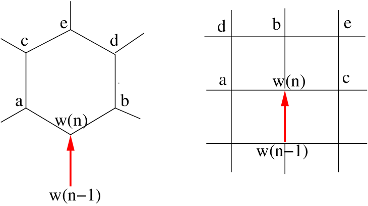
Suppose the walk has been defined for , and let a nearest neighbor of . Since the current site is not a trapping site, in order for to be a trapping site the walk must be close to forming a loop that disconnects from . To determine which sites are trapping sites we need to know which sites are inside and which are outside the loop that is about to be formed. This can be efficiently determined using the winding angle of the loop [10]. We first consider the hexagonal lattice, referring to figure 9. If one of the nearest neighbors or is occupied then the other nearest neighbor cannot be occupied and cannot be a trapping site. So we need only consider the case that neither nearest neighbor is occupied. We describe how we determine if the nearest neighbor is a trapping site. The procedure for is similar. Since is not a trapping site, in order for to be a trapping site, at least one of the sites must be occupied. The portion of the walk from this occupied site to is then close to forming a loop. We can close it to form a loop by adding two or three steps. We do this in such a way that the extension does not pass through . We then compute the orientation of the loop we have formed. This orientation tells us if is inside or outside the loop, and so we can determine if the loop disconnects the nearest neighbor from . If it does then the nearest neighbor is a trapping site. (We note that the process we have just described to form a loop is only to determine which sites are trapping sites. The two or three steps added to form this loop should not be confused with the next step that the walk will take.) Once we have determined which nearest nearest neighbors of are not allowable since they occupied or trapping, we then pick one of the allowable nearest neighbors with equal probability to be .
For the square lattice we refer again to figure 9. Since is not a trapping site, in order for one of the nearest neighbors of to be a trapping site, at least one of the sites must be occupied. For example, if is occupied then one of or must be a trapping site. (Which one depends on how the walk connects to .) If is occupied then it is possible to connect to in such a way that and are trapping sites. However, this connection would mean that is a trapping site. So this case does not happen. Likewise we need not worry about the possibility that being occupied makes and trapping sites. If is occupied then depending on how the walk connects to either will be a trapping site or and will both be trapping sites. Similarly, if is occupied then either is a trapping site or both and are trapping sites. When one of are occupied, we determine which nearest neighbors are forced to be trapping sites by extending the walk one or two steps from to the occupied site in such a way that the walk does not pass through the nearest neighbor in question. The orientation of this loop then determines whether the site is inside the loop. If it is inside it is a trapping site.
To compute the orientation of loops efficiently, as we generate the walk we record the total of the angles of the turns the walk has made up to the current point. Given a loop we can compute the total of the angles of the turns in the loop by taking the difference of two of these totals. This total for the loop tells us the orientation of the loop. In principle the time needed to generate a sample with steps should be , but we have not tested if this is true in practice.
4 Further simulations
In the previous section we assumed that the scaling limit of the SKSAW is rotationally invariant. When we studied the exit distribution for various domains, we used this assumption to average over rotations of the lattice with respect to the domain. This averaging smooths out the discrete nature of the exit distribution and allows for a better comparison with harmonic measure. For the random variables in the disc, we used this rotational invariance to rotate the lattice so that the SKSAW exits the disc at . In this section we do not assume that the scaling limit is rotationally invariant. We carry out two types of simulations that are similar to those of the previous section. All the simulations in this section were only done for the square lattice.

The first set of simulations compute the exit distribution for the same three domains considered in the previous section, but without averaging over the orientation of the lattice. We also compute the exit distribution for a unit disc when the SKSAW starts at the center of the disc and the orientation of the lattice is fixed. If we were to average over orientations of the lattice, then this distribution would trivially be uniform on the boundary. Without the averaging it is not. Checking that it converges to the uniform distribution as the lattice spacing goes to zero serves as a test of the rotation invariance of the scaling limit. For each of the four domains we simulated the SKSAW with lattice spacings of . For each lattice spacing we generated samples. We computed the norm of the difference between the CDF of the exit distributions from the simulations and the CDF of harmonic measure. These norms are plotted as a function of in figure 10. The lines shown are least squares fits to the data.

The second type of simulation in this section studies the random variables from the previous section. We divide the boundary of the disc into six disjoint subsets and condition on the event that the SKSAW exits the disc in one of these subsets. For the walks that meet this conditioning we rotate the lattice so that the walk exits at . Thus for each of the three random variables we have six different distributions corresponding to the subset that we condition on. In the scaling limit we expect that they will converge to the same limit thanks to the rotation invariance. But before the scaling limit these six distributions are clearly different.
The six subsets of the boundary of the disc are defined as follows. Let be the polar angle of the point where the walk exits the disc. For the subsets are defined by dividing into six subintervals of equal length. The rotation and reflection symmetries of the square lattice imply that any outside of is equivalent to an angle in this interval. We extend the six subsets to all of accordingly.
For each random variable and each subset of the boundary we compute the norm of the difference between the CDF of the random variable conditioned on this subset and the predicted CDF. Then for each random variable we sum the six norms corresponding to the six subsets. This gives an overall measure of the deviation of the CDF’s with the conditioning from the prediction. Simulations were done for lattice spacings of . For each we generated samples. So for each subset of the boundary there are approximately as many samples for the conditioned CDF. These sums of norms for the three random variables are plotted as a function of in figure 11. Again, the lines are least squares fits to the data.
5 Conclusions and open questions
We have carried out four types of simulations to test the conjecture that the scaling limit of the smart kinetic self-avoiding walk on the square lattice in the full-plane is full-plane SLE6. In one set of tests we compute the exit distribution for three particular domains under the assumption that the scaling limit is rotationally invariant. We conjecture not only that this distribution converges to harmonic measure, the SLE6 prediction for the distribution, as the lattice spacing goes to zero, but also that the leading order correction is proportional to . Our simulations provide excellent support for this conjecture for both the square and hexagonal lattices.
Our second set of tests look at the full-plane SKSAW up to the time it exits the unit disc centered at the origin. We assume that the scaling limit is rotationally invariant so that we can rotate the disc to put the exit point at . We then compute the distribution of the three random variables and . Their distributions for the analogous process using full-plane SLE6 can be computed explicitly and we find excellent agreement with these predictions. Again we conjecture that the leading order correction is proportional to and find strong support for this prediction for the square lattice.
The third set of tests is the same as the first set of tests except that we do not average over orientations of the lattice. The fourth set of tests is similar to the second set of tests. In the second set we rotated so that the walk exits the disc at . For the fourth set we divide the boundary of the disc into six subsets and condition on the event that the walk exits the disc in one of them, and then rotate the disc so that the walk exits at 1. The third and fourth sets of tests find strong support for the rotational invariance of the scaling limit.
We expect that the SKSAW is in the universality class of the so called -point for polymers. In particular, we expect it to be in the same universality class as the interacting self-avoiding walk given by (1) at its critical point. So if we take the -step ISAW in the full-plane, let and then let , then we expect to get full-plane SLE6. If we want to define the ISAW in a simply connected domain so that the scaling limit is radial or chordal SLE6, then the definition is more subtle. The SKSAW on the hexagonal lattice helps explain what the definition should be. Let be a simply connected domain containing the origin. Consider a full-plane SKSAW from to stopped when it first exits the domain. Let be the SKSAW up to this exit. It can be shown that on the hexagonal lattice the probability of essentially satisfies
where is the number of hexagons which have an edge in . Thus the SKSAW up to the time it exits the domain is equivalent to taking all self-avoiding walks in the domain which start at the origin and end on the boundary and weighting them according to the above equation. The analogous construction for the ISAW is to take all self-avoiding walks in the domain which start at the origin and end on the boundary and weight them by with given by (1). So the scaling limit of this variant of the ISAW is not radial SLE6, but rather full-plane SLE6 stopped when it exits the domain. The energy does not depend on the boundary. The only effect of the boundary is that we only consider walks in from to the boundary.
Now fix a point on the boundary of the domain and consider the radial SKSAW from to . It can be shown that on the hexagonal lattice the probability of a walk in this model essentially satisfies
where is the number of hexagons which have an edge which belongs to not including the hexagons on the boundary. Let be the number of boundary hexagons that have an edge in . So , and thus is proportional to . So the radial SKSAW can be thought of as the full-plane SKSAW conditioned to exit the domain at and weighted so that it is attracted to the boundary. Thus to define a version of the ISAW that would have radial SLE6 as its scaling limit, we would need to include some sort of attractive interaction with the boundary. Presumably we would also need to tune the parameters in the boundary interaction to put the system at an appropriate critical point.
Acknowledgments: An allocation of computer time from the UA Research Computing High Performance Computing (HPC) and High Throughput Computing (HTC) at the University of Arizona is gratefully acknowledged.
References
- [1] D. J. Amit, G. Parisi, L. Peliti, Asymptotic behavior of the “true” self-avoiding walk. Phys. Rev. B 27, 1635 (1983).
- [2] F. Camia, C. M. Newman, Critical percolation exploration path and SLE6 : a proof of convergence. Probab. Theory Related Fields 139,473–519 (2007). Archived as arXiv:math/0605035 [math.PR].
- [3] A. Coniglio, N. Jan, I. Majid, H. E. Stanley, Conformation of a polymer chain at the Theta′ point: connection to the external perimeter of a percolation cluster. Phys. Rev. B 35, 3617 (1987).
- [4] B. Duplantier, H. Saleur, Exact tricritical exponents for polymers at the FTHETA point in two dimensions. Phys. Rev. Lett. 59, 539 (1987).
- [5] M. Gherardi, Theta-point polymers in the plane and Schramm-Loewner evolution. Phys. Rev. E 88, 032128 (2013). Archived as arXiv:1306.4993 [cond-mat.stat-mech].
- [6] J. M. F. Gunn, M. Ortuño, Percolation and motion in a simple random environment. J. Phys. A 18, L1095 (1985).
- [7] J. Jiang, Exploration processes and SLE6. Preprint (2014). Archived as arXiv:1409.6834 [math.PR].
- [8] T. Kennedy, Monte Carlo tests of SLE predictions for 2D self-avoiding walks. Phys. Rev. Lett. 88, 130601 (2002). Archived as arXiv:math/0112246v1 [math.PR].
- [9] T. Kennedy, Conformal invariance and stochastic Loewner evolution predictions for the 2D self-avoiding walk - Monte Carlo tests. J. Stat. Phys. 114, 51–78 (2004). Archived as arXiv:math/0207231v2 [math.PR].
- [10] K. Kremer, J. W. Lyklema, Indefinitely growing self-avoiding walk. Phys. Rev. Lett. 54, 267 (1985).
- [11] G. Lawler, Conformally Invariant Processes in the Plane. American Mathematical Society (2005).
- [12] G. Lawler, The Laplacian- random walk and the Schramm-Loewner evolution. Illinois J. Math. 50, 701–746 (2006).
- [13] G.F. Lawler, O. Schramm, and W. Werner, On the scaling limit of planar self-avoiding walk, Fractal Geometry and Applications: a Jubilee of Benoit Mandelbrot, Part 2, 339, Proc. Sympos. Pure Math. 72, Amer. Math. Soc., Providence, RI, 2004. Archived as arXiv:math/0204277v2 [math.PR].
- [14] G. Lawler, O. Schramm, W. Werner, Conformal Invariance of Planar Loop-Erased Random Walks and Uniform Spanning Trees. Ann. Probab. 32, 939–995, (2004). Archived as arXiv:math/0112234 [math.PR].
- [15] J. W. Lyklema, C. Evertsz, L. Pietronero, The Laplacian random walk. Europhys. Lett. 2, 77 (1986).
- [16] N. Madras and G. Slade, The Self-Avoiding Walk. Birkhäuser (1996).
- [17] I. Majid, N. Jan, A. Coniglio, H. E. Stanley, Kinetic growth walk: A new model for linear polymers. Phys. Rev. Lett. 52, 1257 (1984).
- [18] S.S. Manna, A. J. Guttmann, Kinetic growth walks and trails on oriented square lattices: Hull percolation and percolation hulls. J. Phys. A 22, 3113 (1989).
- [19] S. Smirnov, Critical percolation in the plane: Conformal invariance, Cardy’s formula, scaling limits. C. R. Math. Acad. Sci. Paris 333, 239–244 (2001). Archived as arXiv:0909.4499 [math.PR].
- [20] A. Weinrib, S. A. Trugman, A new kinetic walk and percolation perimeters. Phys. Rev. B 31, 2993 (1985).
- [21] W. Werner, Lectures on two-dimensional critical percolation, Statistical Mechanics (IAS/Park City mathemematics series v. 16), S. Sheffield, T. Spencer (eds.) (2007). Archived as arXiv:0710.0856 [math.PR]
- [22] H. Wu, Conformal restriction: the radial case. Preprint (2013). Archived as arXiv:1304.5712 [math.PR].
- [23] R. M. Ziff, P. T. Cummings, G. Stell, Generation of percolation cluster perimeters by a random walk. J. Phys. A 17, 3009 (1984).