TTP14-026 Two-loop helicity amplitudes for the production of two off-shell electroweak bosons in quark-antiquark collisions
Abstract
Knowledge of two-loop QCD amplitudes for processes is important for improving the theoretical description of four-lepton production in hadron collisions. In this paper we compute these helicity amplitudes for all intermediate vector bosons, , , , , , including off-shell effects and decays to leptons.
I Introduction
Production of vector boson pairs at the LHC is an interesting process for a variety of reasons. For definiteness, let us consider the final state. In that case, ATLAS and CMS collaborations have recently observed that the production cross section is about twenty percent higher than existing theoretical predictions [1, 2, 3]. This observation prompted speculations about the possibility to explain this excess by physics beyond the Standard Model [4] and, at the same time, strongly emphasized the need to improve predictions for production within the Standard Model itself [5, 6]. In addition, production of pairs is an important process for studying anomalous couplings of electroweak gauge boson. Although current limits are already quite impressive [7], it is clear that studies of anomalous gauge boson couplings will intensify once the LHC Run II is underway. Making use of higher experimental precision will require improved modeling of production in the Standard Model. Finally, the process with one -boson on the mass shell and the other off the mass-shell, is an important background to Higgs boson production in channel. Better understanding of this background should allow improved measurements of Higgs boson couplings to -bosons – including the anomalous ones – in the next run of the LHC. Similar arguments can be given for processes with other vector bosons in the final state.
It follows from these examples, that higher theoretical accuracy for vector-boson pair production in hadron collisions is essential. It can be achieved by extending existing computations of cross sections and kinematic distributions of processes [6, 5, 11, 12, 14, 15, 16] to next-to-next-to-leading order (NNLO) in perturbative QCD.11 1 First NNLO QCD results for electroweak boson pair production have recently appeared, see e.g. Refs.[8, 9, 10]. In particular, predictions for fiducial volume cross sections, where kinematic restrictions on final state particles are taken into account exactly, are crucial. A NNLO QCD prediction for needs three ingredients: i) real-emission matrix elements for , and ; ii) one-loop matrix elements for and and, finally, iii) two-loop amplitudes for tree-level process . Once these three ingredients become available, they need to be put together in a self-consistent manner using existing methods for fully differential NNLO computations [17]. For the production, the major unknown is the two-loop amplitude for ; the goal of this paper is to provide it.
The remainder of the paper is organized as follows. In Section II we explain the general setup of the calculation. Since two-loop scalar master integrals required for this computation have been recently computed for equal electroweak boson masses in Refs. [18, 19] and for unequal masses in Refs. [21, 20], we mainly focus on the procedure that allows us to express the various contributions to scattering amplitudes in terms of these integrals. In Section III we describe checks on our computation, evaluate the scattering amplitudes numerically and discuss numerical stability of the results. We conclude in Section IV.
II The setup of the computation
We are interested in the production of a four-lepton final states in proton collisions . The four-lepton final states can be produced in three distinct ways:
- •
through the production of a pair of off-shell vector bosons, ;
- •
through the production of a single vector boson that decays to two vector bosons that, in turn, decay to lepton pairs, ;
- •
through the production of a single vector boson that decays into a pair of leptons (one of them of-shell), followed by the emission of a vector boson by an of-shell lepton, e.g. .
Each of these three processes depends on different combinations of electroweak couplings; therefore, they are separately invariant under QCD gauge transformations and we can compute QCD corrections to each of them separately. We note in this respect that QCD corrections to processes mediated by single gauge-boson production are simple since they are directly related to QCD corrections to the quark form factor of the vector current whose perturbative expansion through NNLO is well-known [22].
However, computation of NNLO QCD corrections to process , where vector bosons couple only to fermions and not to other vector bosons or primary leptons, is non-trivial. Calculation of this contribution to two-loop QCD amplitudes for four-lepton production processes is the main focus of this paper.
We consider quark-antiquark annihilation in to vector bosons
| (1) |
and work in the approximation where quarks of the first two generations are massless and quarks of the third generation are consistently neglected. We also set the CKM matrix to an identity matrix. Since we work with massless quarks, helicity is a conserved quantum number; therefore, once the helicity of the incoming quark is specified, the helicity of the incoming anti-quark is completely fixed. We will use this observation when writing the amplitude for quark-antiquark annihilation process in Eq.(1).
The partonic process in Eq.(1) can proceed in two different ways since the vector bosons can either couple directly to external fermions or to closed loops of virtual fermions, see Fig.1. Consequently, we write the scattering amplitude for process in Eq.(1) as
| (2) |
where is the weak coupling, is the -boson propagator, are helicities of the incoming quark and outgoing leptons, respectively, and are helicity-dependent couplings of vector bosons to quarks and leptons, and are matrix elements for leptonic decays of and that we will specify shortly. The amplitudes describe direct coupling of the vector bosons to external fermions and the amplitude describes contributions of diagrams where vector bosons couple to loops of virtual fermions, see Fig. 1. The factor involves sums over couplings of virtual fermions to gauge bosons.
We note that full amplitude for in Eq.(2) is written as the sum of two amplitudes where two vector bosons appear in different order. These amplitudes are, therefore, quantities similar to ordered or primitive amplitudes often used in perturbative QCD computations. For us they are useful because we only need to compute one of them and then obtain the other one from permutation. We stress that amplitudes and in Eq.(2) are computed assuming that vector bosons couple to a single quark generation and that the coupling is vector-like with unit coefficient, i.e. . As we explain below, such amplitudes are sufficient to obtain physical amplitudes for pair production of all electroweak gauge bosons.

We begin by discussing the parametrization of amplitude in terms of Lorentz-invariant form factors. A representative diagram that contributes to at two loops in perturbative QCD is shown in Fig. 1. Our goal is to re-write these diagrams in such a way that all Feynman integrals can be dealt with using the integration-by-parts technique [23]. To achieve this goal, we need to express the amplitude in terms of invariant form factors. To this end, we note that the most general form of is
| (3) |
where and the vector is defined by the Sudakov decomposition of the momenta
| (4) |
The transverse momentum is orthogonal to , . The coefficients and in Eq.(4) can be written as
| (5) |
where we defined , and introduced standard Mandelstam variables . The functions , introduced in Eq.(3), depend on momenta and Lorentz indices. To make this dependence explicit, we decompose them into invariant form factors ,
| (6) |
We note that not all invariant form factors that appear in Eq.(6) give independent contributions to physical amplitudes. This happens because we did not use the transversality condition for lepton currents . As we will see shortly, when physical amplitudes are computed, the number of relevant form factors will be reduced thanks to the transversality condition.
To calculate the physical amplitude in Eq.(2), we need to contract with polarization vectors of external vector bosons. As we already mentioned, they are given by matrix elements of the vector current between relevant leptonic states. Using the spinor-helicity formalism, we write
| (7) |
Since, as we already pointed out, the helicity of the incoming quark fully determines the allowed helicity of the incoming antiquark, we need eight helicity amplitudes to fully describe production of two vector bosons. They are , , , , , , , . We note that, according to Eq.(7), a change in lepton helicities can be obtained by interchanging momenta and , where necessary. Therefore, we obtain all required helicity amplitudes from and by simple permutations of lepton momenta.
For left- and right-handed incoming quarks we find
| (8) |
where the following nine combinations of form factors enter
| (9) |
We note that form factors only depend on and ; therefore, they are invariant under and permutations. For this reason, it is straightforward to obtain all the relevant amplitudes from Eq.(8). To find and , we need to construct projection operators. To accomplish this, we write a generic amplitude as a matrix element of a string of Dirac matrices
| (10) |
Multiplying it with and summing over spinor helicities, we find
| (11) |
Choosing different operators , we can project on individual form factors or their combinations. Below we list all the projection operators and the results that we get when these operators are convoluted with the amplitude
| (12) |
Each of the projections can be calculated from Feynman diagrams by taking traces and integrating over loop momenta. These quantities depend on the Mandelstam invariants of the underlying process but not on the polarization vectors of electroweak bosons or on the momenta of final-state leptons. Thus, they can be expressed in terms of Feynman integrals of the type introduced in Refs. [21, 20] and then reduced to master integrals using integration-by-parts identities.
We can use projections to derive the form factors; the result reads
| (13) |
The form factors that are used for the evaluation of the amplitude can now be easily computed using Eq.(9). We do not present these results here since they are not very illuminating.
One point worth emphasizing though is that in Eq.(13) there are expressions (see e.g. equation for ) that appear to have spurious singularities in the limit . It would have been unfortunate if these singularities survive in the final formulas for form factors since, in such a situation, computation of all pieces needed for the evaluation of ’s, including master integrals, to higher orders in is required. It is therefore pleasing to observe that this does not happen and once results for the form factors are written in terms of projectors, all spurious singularities disappear.
For future reference, we give results for leading order form factors that appear in the physical amplitudes Eq.(8)
| (14) |
We stress that these results are exact in a sense that no limit was taken to obtain them; in other words, all the -dependence cancels out completely once physical form factors are computed.
Before proceeding to the discussion of various couplings of vector bosons to fermions introduced in Eq.(2), we want to explain why and amplitudes can be computed assuming that interactions of vector bosons with quarks are mediated by vector currents. The main reason is that we only consider here contributions of massless quarks and that, in such a case, the helicity is conserved. Therefore, we can always write couplings of vector bosons to fermions as linear combinations of left- and right-handed couplings and then move helicity projection operators to external lines. In this way the helicity-dependent couplings are generated and amplitudes that remain can be viewed as originating from pure vector current interactions of gauge bosons and quarks.
Of course, this discussion applies only to diagrams where vector bosons couple directly to external quark lines; in the notation of Eq.(2) such diagrams contribute to amplitudes. However, we will now argue that the same parametrization Eq.(3) can be used to compute amplitudes , which receive contributions from diagrams where vector bosons couple to closed fermion loops. In fact, this would have been obvious provided that electroweak boson coupling to fermions is vector-like since in this case tracing over spin degrees of freedom in the internal quark loop gives us diagrams that are not very different from the ones that we already considered. Potential problems could be expected with axial couplings and, in particular, with terms where one axial and three vector couplings appear in Green’s function. However, all such terms cancel because of -parity conservation for massless fermions for any final state with two vector bosons [15].22 2 More precisely, for -parity argument to be applicable, all fermions in the loop should have equal masses [15]. Contributions of terms with two vector and two axial couplings are not anomalous and must be equal to those with four vector couplings. Hence, we conclude that it is sufficient to consider vector-current couplings of gauge bosons to internal fermion loops, to account for all non-vanishing contributions to the amplitude. The parametrization of the amplitude is then taken from Eq.(3) and its expression through invariant form factors is taken from Eq. (8).
To complete our construction of the scattering amplitude for in Eq.(2), it remains to specify various helicity-dependent couplings that we introduced there. Below we present these couplings for various pairs of electroweak gauge bosons that can be produced in proton collisions.
II.1 production
Photons are produced in the annihilation of a quark and an antiquark of the same flavor . Photon interactions with both quarks and leptons are pure vector-like and, therefore, helicity-independent. We find
| (15) |
where and are electromagnetic quark and lepton charges in units of the positron charge. Finally, is given by the sum of up and down quark charges of the first two generations
| (16) |
II.2 production
Pairs of bosons are produced in annihilation of quarks and anti-quarks of the same flavor. Couplings of bosons to quarks and leptons depend on helicity and weak isospin of the corresponding particle. We find
| (17) |
where
| (18) |
The coefficient is given by the sum of up and down quark vector and axial charges of the first two generations. We find
| (19) |
II.3 production
II.4 and for production
The final state is produced in annihilation, . Production of occurs in process. Since bosons interact with left-handed fermions, we have
| (21) |
Coefficients and vanish identically due to electric charge conservation.
II.5 and for production
Production processes for are identical to . The relevant couplings are
| (22) |
Coefficients vanish identically due to electric charge conservation.
II.6 production
Finally, we display the necessary couplings for the pair production of two bosons. This process can occur thanks to and annihilation. First, consider the process . In this case,
| (23) |
In case of , the coupling constants read
| (24) |
Couplings to leptons are given in Eq.(22). The coefficient receives contributions from two generations33 3 As we already mentioned several times, we do not consider the third quark generation in this paper. and reads
| (25) |
III Calculation of the form factors and the amplitudes
Once projection operators are established, one can compute the form factors and construct the scattering amplitudes for arbitrary di-boson final state. To this end, we note that all integrals that appear in the calculation of form factors can be associated with one of the six topologies, introduced in Refs. [21, 20]. Integrals that belong to each of these topologies are closed under the integration-by-parts identities [23]. We use QGRAF [25] to generate Feynman diagrams and FORM [26] for algebraic manipulations and computation of projections . We use FIRE [27, 28, 29] to reduce all the integrals that appear in this calculation to master integrals. The master integrals were computed by us in Refs. [21, 20]. In principle, once all the ingredients are in place, computation of the amplitude becomes straightforward. In practice, however, it requires some effort to put all the pieces together primarily because algebraic expressions that appear e.g. in the course of the reduction to master integrals are quite large in size. The master integrals are expressed in terms of Goncharov polylogarithms up to weight four; we use GiNaC [30] implementation [31] to compute them.
The results for the amplitudes contain infra-red and ultraviolet divergences. The ultraviolet divergences are removed by the renormalization of the strong coupling constant. Since tree-level scattering amplitudes are independent of , we only need its renormalization through one loop. It reads
| (26) |
where is the bare and is the renormalized coupling constant. In addition, is the QCD beta-function, is the number of massless flavors, and , with being the Euler constant.
According to Catani [32], infra-red singularities of UV-renormalized amplitudes at next-to-next-to-leading order are fully determined by leading and next-to-leading order amplitudes. This feature can be used as an important check of the correctness of the computation. To introduce Catani’s result, we write a UV-renormalized amplitude as
| (27) |
Leading order amplitude in this formula is finite and, in fact, -independent. The next-to-leading order amplitude contains infra-red divergences that, however, can be written in a factorized form
| (28) |
For the process of vector boson pair production, the final state is neutral. Therefore,
| (29) |
where and . In variance with , and depend on the dimensional regularization parameter . This feature is important for proper comparison of Catani’s formula with results of explicit computation.
| Helicity | |||||
|---|---|---|---|---|---|
The two-loop amplitude can be written in a similar way
| (30) |
where
| (31) |
The two constants that enter this formula read
| (32) |
We note that Catani formula can also be used for individual form factors that we introduced earlier to describe physical amplitudes. To this end, we only need to replace tree and loop amplitudes in the above formulas with the corresponding form factors. We have used the above results for the infra-red poles of scattering amplitudes to check the correctness of our computation of the amplitudes . We also note that the amplitude appears for the first time at NNLO; therefore, according to Catani’s formula it cannot have infra-red singularities. This is an important check of the correctness of the computation of the amplitude .
| Helicity | |||||
|---|---|---|---|---|---|
We turn to the discussion of numerical results for the scattering amplitudes , . We define those amplitudes by contracting them with polarization vectors of electroweak bosons
| (33) |
and write their perturbative expansion as
| (34) |
where . We note that in Eq.(34) we choose to expand in bare, rather than renormalized, QCD coupling. Also, we made it explicit in Eq.(34) that the amplitude appears at two loops for the first time.
To motivate our choice of kinematics for numerical results for the amplitudes that we present below, we consider production as the background to Higgs boson signal in . Therefore, we choose the center-of-mass energy to be the mass of the Higgs boson . The invariant mass of the vector boson is set to , with . The invariant mass of the second vector boson is set to . We take the vector boson scattering angle in the center-of-mass collision frame to be radians. We also take decay angles of the lepton in the rest frame of the boson to be and and decay angles of the lepton in the rest frame of the boson to be and . The four-momenta of initial and final state particles are given by
| (35) |
To obtain numerical results for the amplitude, we take the number of massless fermion species to be five. Results for selected helicity amplitudes and are shown in Tables 1,2,3. They can be compared to predictions based on Catani’s formula44 4 Catani’s formula needs to be re-written to provide an expansion in the unrenormalized QCD coupling.. For both one- and two-loop amplitudes, divergent terms agree perfectly. For the one-loop amplitudes, we can also compare the terms against the known results [33]; we find perfect agreement. The amplitude that describes contributions to where vector bosons couple to closed loops of fermions is finite as expected since those amplitudes have no tree- and one-loop contributions.
| Helicity | |||||
|---|---|---|---|---|---|
We will now elaborate on the numerical stability of our results. This is an important issue since amplitudes for vector boson pair productions may exhibit numerical instabilities in the limit of forward or backward scattering. In fact, numerical stability depends on the vector boson transverse momentum since singularities appear when Feynman integrals are reduced to master integrals. We have evidence from previous studies about values of transverse momenta where such instabilities arise. In case of one-loop amplitudes, numerical instabilities start to appear for transverse momenta of an order of a few GeV [34, 35] and sophisticated treatment is required to remove them completely [35]. To explore numerical (in)stability of our results, we study amplitudes in dependence of the vector boson scattering angle. All other kinematic variables are taken to be identical to what we described above.
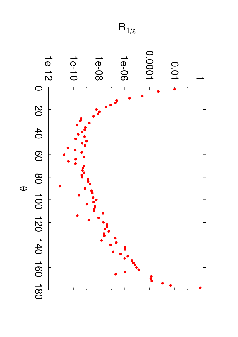
In Fig. 2 we show ratios of singularities in the squared amplitude computed directly and using Catani’s formula. Deviations of this ratio from one signal numerical instabilities. We observe that is of order in the bulk of the phase-space. Significant instabilities are observed for backward scattering ( degrees), where the transverse momentum is close to . However, the situation improves considerably already for degree scattering where the transverse momentum is . The forward scattering limit appears to be more stable; even at two degrees, the contribution is computed properly to within a percent.
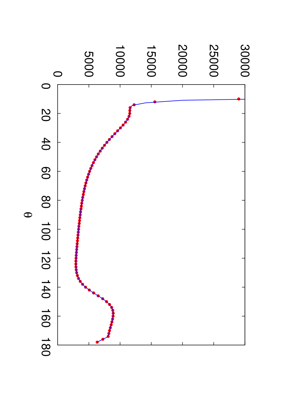
;
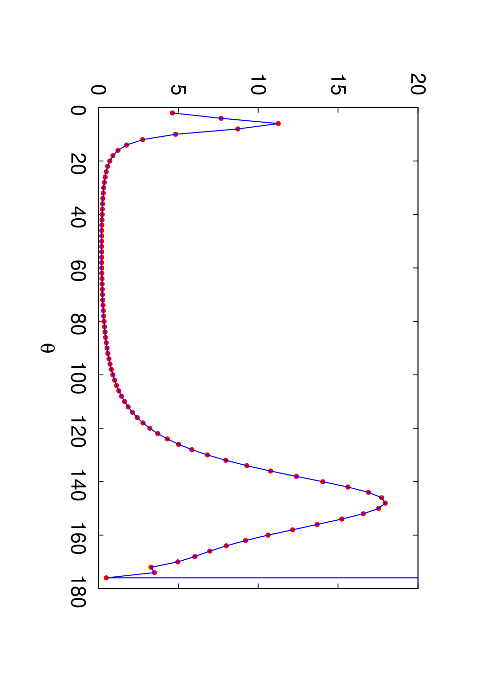
In the left pane of Fig. 3 we show the absolute value squared of the ratio of the finite part of the amplitude and the leading order amplitude . To understand numerical accuracy of these results, we compared the output obtained with the double-precision version of the Fortran code with the Mathematica implementation. The advantage of the latter is that it provides a possibility to compute amplitudes with arbitrary numerical precision thereby ameliorating the problem of numerical instability. For backward scattering, we find that up to degrees, the finite part is computed to within a per mille. For forward direction, the situation is similar but, perhaps, slightly better.
Finally, in the right pane of Fig. 3 we show absolute value squared of the ratio of the finite part of the left amplitude and the leading order amplitude . Numerical instabilities are apparent for backward scattering. In fact, at degrees (), the agreement between double-precision Fortran code and the Mathematica code is about ten percent. In the forward direction, the situation is much better – the double-precision Fortran results agree with the results obtained using Mathematica implementation to better than a fraction of a percent for scattering angles as small as six degrees.
To summarize, while the two-loop amplitudes that we compute in this paper do exhibit numerical instabilities at small values of vector boson transverse momenta, we believe the stability is acceptable for phenomenological applications. Moreover, there are several ways to improve the situation. For example, it is possible to extend the Fortran code to provide results with quadruple precision. Note that computation of master integrals with arbitrary precision is feasible since Goncharov polylogarithms implementation in GiNaC does provide this functionality [31]. Moreover, it should also be possible to construct expansion of analytic expressions for scattering amplitudes that we obtained in this paper around singular limits, for example for forward or backward scattering and threshold production. If such expansions become available, computation of helicity amplitudes in singular limits will be significantly simplified. We leave these improvements for future work.
IV Conclusions
In this paper we described computation of two-loop scattering amplitudes for the annihilation of a quark and an antiquark into four leptons, that occurs through the production of two electroweak gauge bosons. The invariant masses of gauge bosons are kept arbitrary. We have given explicit formulas for projection operators that allow one to compute contributions of individual Feynman diagrams to invariant form factors. We use these form factors to construct helicity amplitudes for vector boson pair production processes including all off-shell effects and leptonic decays of vector bosons.
Results for two-loop scattering amplitudes obtained in this paper remove the last obstacle for computing the NNLO QCD corrections to the production of pairs of vector bosons with identical and different invariant masses. The two-loop virtual corrections that we compute in this paper will have to be combined with one-loop amplitudes for and with tree amplitudes for . While doing this consistently is non-trivial, the relevant technology is well-understood by now [17]. We hope, therefore, that results for NNLO fiducial volume cross sections for pair production of electroweak bosons can be expected in the near future.
V Acknowledgments
J.M.H. and A.V.S. are grateful to Institute for Theoretical Particle Physics (TTP) at Karlsruhe Institute of Technology for the hospitality extended to them during the work on this paper. Research of K.M and F.C. was partially supported by US NSF under grant PHY-1214000. K.M. was also partially supported by Karlsruhe Institute of Technology through its distinguished researcher fellowship program. J.M.H. is supported in part by the DOE grant DE-SC0009988 and by the Marvin L. Goldberger fund. F.C. and A.S. are supported in part by DFG through SFB/TR 9. V.S. is supported in part by the Alexander von Humboldt Foundation (Humboldt Forschungspreis).
Note added In the original version of this paper, one of the form factors that contributes to the amplitude was calculated incorrectly. We are grateful L. Tancredi for pointing this out to us. After correcting this mistake, our results for the two-loop amplitudes agree with the results of an independent calculation in Ref. [36].
References
- [1] G. Aad et al. ATLAS collaboration, Phys. Rev. D87, (2013), 112001 [Erratum ibid., 88, (2013) 079906].
- [2] CMS Collaboration, CMS-PAS-SMP-12-005.
- [3] CMS Collaboration, CMS-PAS-SMP-12-013.
- [4] D. Curtin, P. Meade, P.J. Tien, arXiv:1406.0848; D. Curtin, P. Jaiswal, P. Meade, Phys. Rev. D 87 (2013) 031701.
- [5] P. Meade, H. Ramani and M. Zeng, arXiv:1407.4481 [hep-ph].
- [6] P. Jaiswal and T. Okui, arXiv:1407.4537 [hep-ph].
- [7] For recent results and earlier references, see e.g. CMS Collaboration, hep-ex/1406.0113; CMS collaboration Phys. Rev. D89 (2014) 092005, ATLAS collaboration, Phys. Lett. B 717 (2012) 49.
- [8] F. Cascioli, T. Gehrmann, M. Grazzini, S. Kallweit, P. Maierhöfer, A. von Manteuffel, S. Pozzorini, D. Rathlev, L. Tancredi and E. Weihs, arXiv:1405.2219 [hep-ph].
- [9] Ch. Anastasiou, J. Cancino, F. Chavez, C. Duhr, A. Lazopoulos, B. Mistlberger and R. Mueller, arXiv:1408.4546 [hep-ph].
- [10] T. Gehrmann, M. Grazzini, S. Kallweit, P. Maierhöfer, A. von Manteuffel, S. Pozzorini, D. Rathlev, L. Tancredi, arXiv:1408.5243 [hep-ph].
- [11] J. Ohnemus and J. F. Owens, Phys. Rev. D 43 (1991) 3626; J. Ohnemus, Phys. Rev. D 44 (1991) 3477; J. Ohnemus, Phys. Rev. D 44 (1991) 1403; B. Mele, P. Nason and G. Ridolfi, Nucl. Phys. B 357 (1991) 409; S. Frixione, P. Nason and G. Ridolfi, Nucl. Phys. B 383 (1992) 3; S. Frixione, Nucl. Phys. B 410 (1993) 280; U. Baur, T. Han and J. Ohnemus, Phys. Rev. D 53 (1996) 1098; L. J. Dixon, Z. Kunszt and A. Signer, Phys. Rev. D 60, 114037 (1999); J. M. Campbell and R. K. Ellis, Phys. Rev. D 60 (1999) 113006; J. M. Campbell, R. K. Ellis and C. Williams, JHEP 1107, 018 (2011).
- [12] S. Frixione and B. R. Webber, JHEP 0206 (2002) 029; P. Nason and G. Ridolfi, JHEP 0608 (2006) 077; K. Hamilton, JHEP 1101 (2011) 009; T. Melia, P. Nason, R. Rontsch and G. Zanderighi, JHEP 1111 (2011) 078; R. Frederix, S. Frixione, V. Hirschi, F. Maltoni, R. Pittau and P. Torrielli, JHEP 1202 (2012) 099; F. Cascioli, S. Höche, F. Krauss, P. Maierhöfer, S. Pozzorini and F. Siegert, JHEP 1401 (2014) 046; F. Campanario, M. Rauch and S. Sapeta, Nucl. Phys. B 879 (2014) 65.
- [13] M. Billoni, S. Dittmaier, B. Jäger and C. Speckner, JHEP 1312 (2013) 043; A. Bierweiler, T. Kasprzik, H. Kühn and S. Uccirati, JHEP 1211 (2012) 093; A. Bierweiler, T. Kasprzik and J. H. Kühn, JHEP 1312 (2013) 071; J. Baglio, L. D. Ninh and M. M. Weber, Phys. Rev. D 88 (2013) 113005.
- [14] M. Grazzini, JHEP 0601 (2006) 095; S. Dawson, I. M. Lewis and M. Zeng, Phys. Rev. D 88 (2013) 5, 054028; Y. Wang, C. S. Li, Z. L. Liu, D. Y. Shao and H. T. Li, Phys. Rev. D 88 (2013) 114017.
- [15] E.W.N. Glover and J.J. van der Bij, Phys. Lett. B 219, (1989) 488; G. Kao and D.A Dicus, Phys. Rev. D 43, (1991), 1555.
- [16] T. Binoth, M. Ciccolini, N. Kauer and M. Krämer, , JHEP 0503 (2005) 065; T. Binoth, M. Ciccolini, N. Kauer and M. Krämer, JHEP 0612 (2006) 046.
- [17] A. Gehrmann-De Ridder, T. Gehrmann and E. W. N. Glover, JHEP 0509, 056 (2005); S. Catani and M. Grazzini, Phys. Rev. Lett. 98, 222002 (2007); S. Catani, L. Cieri, D. de Florian, G. Ferrera and M. Grazzini, Nucl. Phys. B 881, 414 (2014); S. Weinzierl, JHEP 0303, 062 (2003); G. Somogyi, P. Bolzoni and Z. Trocsanyi, Nucl. Phys. Proc. Suppl. 205-206, 42 (2010) and references therein. M. Czakon, Phys. Lett. B 693, 259-268 (2010); M. Czakon, Nucl. Phys. B 849, 250-295 (2011); M. Czakon and D. Heymes, arXiv:1408.2500 [hep-ph]; R. Boughezal, K. Melnikov and F. Petriello, Phys. Rev. D 85, 034025 (2012).
- [18] T. Gehrmann, A. von Manteuffel, L. Tancredi and E. Weihs, JHEP 1406, 032 (2014).
- [19] T. Gehrmann, L. Tancredi and E. Weihs, JHEP 1308, (2013) 070;
- [20] F. Caola, J. M. Henn, K. Melnikov, V. A. Smirnov, arXiv:1404.5590.
- [21] J. M. Henn, K. Melnikov and V. A. Smirnov, JHEP 1405 (2014) 090.
- [22] R.J. Gonsalves, Phys. Rev. D 28 (1983) 1542; W.L. van Neerven, Nucl. Phys. B 268 (1986) 453; G. Kramer and B. Lampe, J. Math. Phys. 28 (1987) 945.
- [23] F. Tkachov, Phys. Lett. B 100 (1981) 65; K.G. Chetyrkin and F. Tkachov, Nucl. Phys. B 192 (1981) 159.
- [24] J.M. Henn, Phys. Rev. Lett. 110 (2013), 251601.
- [25] P. Nogueira, J.Comput.Phys. 105 (1993) 279.
- [26] J. Kuipers, T. Ueda, J. Vermaseren, and J. Vollinga, Comput.Phys.Commun. 184 (2013) 1453.
- [27] A. V. Smirnov, JHEP 0810 (2008) 107.
- [28] A. V. Smirnov and V. A. Smirnov, Comput. Phys. Commun. 184 (2013) 2820.
- [29] A. V. Smirnov, arXiv:1408.2372 [hep-ph].
- [30] C. W. Bauer, A. Frink and R. Kreckel, cs/0004015 [cs-sc].
- [31] J. Vollinga and S. Weinzierl, Comput. Phys. Commun. 167 (2005) 177.
- [32] S. Catani, Phys. Lett. B 427 (1998) 161.
- [33] L. J. Dixon, Z. Kunszt and A. Signer, Nucl. Phys. B 531 (1998) 3;
- [34] N. Kauer and G. Passarino, JHEP 1208 (2012) 116.
- [35] J. M. Campbell, R. K. Ellis and C. Williams, JHEP 1404 (2014) 060.
- [36] T. Gehrmann, A. von Manteuffel, L. Tancredi, arXiv:1503.04812.