A Simulation Approach for Change-Points on Phylogenetic Trees

Several negative mathematical results exist in the literature (e.g. [23]) for Markov chain Monte Carlo (MCMC) inference when the tree topology (and branch lengths) is unknown, and these have spurred the development of highly sophisticated Monte Carlo-based algorithms [24]. Here, the tree topology and branch lengths are assumed to be known, but the position and number of change-points for the rates are unknown. In addition, as we will explain later, the cost of evaluating the likelihood will be an $\mathcal{O}(mp^{2}n^{2})$ operation ($p$ is the number of states at each site, $m$ the number of sites and $n$ the number of sequences). It follows that parameter inference requires expectations w.r.t. a probability on a trans-dimensional state-space. Contructing efficient MCMC algorithms on trans-dimensional spaces is a notoriously challenging problem and the standard approach is to use reversible jump MCMC (RJMCMC) [25]. Typically, and especially for our model, it is difficult to develop moves on the trans-dimensional state-space that are likely to be accepted, which is important here because likelihood computations are expensive.

To deal with some of these inferential and computational issues, we propose:

• •

  To reduce the cost of computing the likelihood and assist the mixing of MCMC, through a likelihood approximation based on the time-machine principle [26].

• •

  To improve mixing compared to standard RJMCMC, by adapting an idea in [27], developing a particle marginal Metropolis-Hastings (PMMH) algorithm [28], based on the sequential Monte Carlo (SMC) samplers method in [29]. This approach can benefit from the time-machine approach.

In the time-machine approach, the unobserved sequence at the root, and possibly also other top-most nodes of the tree, are replaced with the stationary distribution of the substitution process. This can reduce the cost of computing the likelihood by a linear factor in $n$; this can allow larger datasets than would otherwise be manageable. The resulting estimates are biased, but in the examples below we find the bias to be smaller than for competitive methods. Indeed, we conjecture (and this is supported by empirical results) that our approach is competitive with other approximate methods, in particular approximate Bayesian computation (ABC); this latter method is often not appropriate for model selection problems as we describe in Section 3.3. An important point here is that the time-machine performs a ‘principled’ approximation of the mathematical model. This is based on the general understanding that most of the information in the data is at the lower part of the tree, thus contrasting with an often ad-hoc selection of summary statistics in ABC approaches.

Our PMMH algorithm extends the idea in [27], both with regard to the methodology and the context of phylogenetic trees with change-points. The MCMC method will often generate (as we will explain in Section 3.2) trans-dimensional proposals which are more likely to be accepted than standard RJMCMC algorithms. This is further aided by using the time-machine, which results in a less complex posterior with a faster likelihood evaluations. The combination of the above factors can lead to reliable, but biased, inference from moderate sized data-sets. As mentioned above, we expect the bias to be minimal relative to ABC methods.

This article is structured as follows. In Section 3 the model and methods are described; this includes our mathematical result on the bias. In Section 4 our empirical results are given. In Section 5 we conclude the article with a discussion. The appendix provides further details of the methods.

We observe $n$ sequences of length $m$, such that each observation is $x_{ij}\in\{1,\dots,p\}$ with $1\leq i\leq n$, $1\leq j\leq m$. Similar to as in [30], it is assumed that the data originate from a rooted binary tree [2, Chapter 1] of known topology and branch lengths with the $n$ leaves being the observed sequences. The sequences at the other $n-1$ nodes are unobserved. Nodes are numbered backwards in time, starting from the observed leaves (numbered 1 to $n$) to the root $2n{-}1$. Let $\nu:[2n-2]\rightarrow\{n{+}1,\ldots,2n-1\}$ map nodes other than the root onto their parent node. It is assumed that we are given a Markov model on the tree describing the evolution of states over time on each branch of the tree and at each site; each site evolves independently given the branch lengths. Treating the sequence states at internal nodes as missing data we can write the full-data likelihood as:

where $\theta\in\Theta\subseteq\mathbb{R}^{d}$ is an unknown parameter, $f_{\theta}$ a Markov transition probability, and $\mu_{\theta}$ a probability distribution on the state space at a site. Note that $x_{n+1:2n-1,1:m}$ are unobserved, whereas $x_{1:n,1:m}$ are observed. Note also that $f_{\theta}(x_{ij}|x_{\nu(i)j})$ can depend on the (known) length of the branch connecting the node $i$ with node $\nu(i)$. For convenience in subsequent formulas we will write $f_{\theta}(x_{(2n-1)j}|x_{\nu(2n-1)j})$ in place of $\mu_{\theta}(x_{(2n-1)j})$, even though $\nu(2n{-}1)j$ is undefined.

The observed-data likelihood can be written as a sum over the missing data:

Using belief propagation [31] (also called the sum and products algorithm), the cost of computing (2) is $\mathcal{O}(mp^{2}n^{2})$.

Our model generalises (1) to allow $\theta$ to vary along the sequence at a set of change-points $1=s_{0}<s_{1}<\cdots<s_{k+1}=m$. Then the full-data likelihood for the change-point model is:

and, as in (2), one can sum over $x_{n+1:2n-1,1:m}$ to obtain an observed-data likelihood:

where

In order to sample from the trans-dimensional state-space of (3) we first consider an SMC sampler which only samples on $\mathsf{S}_{k}\times\Theta^{k+1}$, for $k$ fixed. We then show how the SMC sampler can be embedded within a PMMH algorithm to target (3). The SMC sampler will be necessary to ensure a good acceptance probability for trans-dimensional moves. Our approach has the advantage over alternative simulation techniques for model selection (see [33]) that the model selection and parameter estimates are simultaneous, which helps to focus computational resources on the important model(s).

For $1\leq k<m$, and a user-specified $T\geq 1$, let $\{\xi_{t,k}\}_{0\leq t\leq T}$ be a sequence of probabilities on $\mathsf{S}_{k}\times\Theta^{k+1}$, such that $\xi_{0,k}(s_{1:k},\theta_{1:k+1})=p(s_{1:k},\theta_{1:k+1}|k)$ and

The remaining sequence of targets $\{\xi_{t,k}\}_{1\leq t\leq T-1}$ interpolate between the (conditional) posterior and the prior, e.g. via the tempering procedure:

with $0<\kappa_{1}<\cdots<\kappa_{T-1}<1$. The SMC sampler will propagate a collection of $N$ particles from the prior $\xi_{0,k}$ all the way to the posterior $\xi_{T,k}$ via the bridging densities $\xi_{t,k}$ by means of importance sampling, resampling and MCMC move steps. The tempering procedure aims at controlling the variability of the incremental importance weights, for instance providing robust estimates of the normalising constants $p(x_{1:n,1:m}|k)$ which is an important attribute for the overall algorithm. The sampler propagates the particles by using a sequence of MCMC kernels of invariant densities $\xi_{t,k}$ (which operate on a fixed dimensional space). All the details of the specific steps of the SMC sampler are given in the Supporting Information document. We write the probability of all the variables associated to the SMC sampler (which resamples $N>1$ ‘particles’ at every time except at time $T$) as

where $a_{0:T-1}^{1:N}=(a_{0}^{1},\dots,a_{0}^{N},\dots,a_{T-1}^{1},\dots,a_{T-1}^{N})$ are the resampled indices and $\phi_{0:T}^{1:N}(k)=(\phi_{0}^{1}(k),\dots,\phi_{0}^{N}(k),\dots,\phi_{T}^{1}(k),\dots,\phi_{T}^{N}(k))$ with $\phi_{t}^{i}(k)=(s_{t,1:k}^{i},\theta_{t,1:k+1}^{i})$, $i\in[N],t\in\{0\}\cup[T]$, is the collections of the $N$ particles as propagated through the sequence $\xi_{t,k}$.

One can use this SMC sampler within a broader PMMH algorithm to sample from the true target of interest (3). The specific steps of PMMH are given in the Supporting Information document, but briefly, a single iteration of the algorithm is as follows. Given the current state of the Markov chain, one proposes to change $k$ with some proposal kernel $q(k^{\prime}|k)$. Conditional on this $k^{\prime}$, we run an SMC sampler $\Psi_{k^{\prime},N}(\cdot)$ and choose a particle $\phi_{T}^{l}(k^{\prime})$, for some $1\leq l\leq N$, with probability proportional to a weight. Acceptance of both the model index $k^{\prime}$ and of the proposed change-point times and rates $\phi_{T}^{l}(k^{\prime})$ happens with probability

where $p^{N}(x_{1:n,1:m}|k)$ is the SMC (unbiased) estimate of $p(x_{1:n,1:m}|k)$, the normalizing constant of $\xi_{T,k}$. The Supporting Information document presents the formula used to calculate $p^{N}(x_{1:n,1:m}|k)$. Note that whilst there are a lot of user set parameters (namely, the temperatures and tuning parameters for the MCMC kernels), their choice can be done adaptively to reduce user involvement (see [34]). In this article we tune the parameters by trial and error.

The advantages of our procedure is that it mitigates having to construct trans-dimensional proposals which need to mix well (see [27] for another recent work that attempts to deal with this issue). We note, however, that the cost of each proposal will be $\mathcal{O}(NTmp^{2}n^{2})$, as $\xi_{t,k}$ must be obtained at each time step of the SMC sampler (see Supporting Information). In addition, note that tailored methods for change-point models (e.g. [35]) do not apply here as one does not have a convenient way to integrate the likelihood.

ABC is another methodology that avoids exact computation of the likelihood, at the cost of a biased approximation of the posterior; see for instance [36] for a review. The method is based on accepting simulated data sets that are similar to the observed dataset, where ‘similar’ is usually assessed using summary statistics sensitive to the parameter(s) of interest.

ABC can be unreliable as a tool for model selection. According to [37], the best summary statistics to be used in ABC approximation to a Bayes factor are ancillary statistics with different mean values under two competing models. Otherwise, the summary statistic must have enough components to prohibit a parameter under a wrong model from generating summary statistics that are plausible under the true model. However, summary statistics satisfying the conditions of [37] for model choice in ABC is not easy (or even possible) to verify in our context.

In the numerical examples of Section 4.1, we consider two ABC algorithms which approximate the same ABC posterior. The first algorithm is a PMMH that replaces the SMC sampler of [29] with the SMC sampler of [38, Section 3.3]; see Supporting Information for details. The second ABC algorithm is the ABC-SMC algorithm for model selection appearing on [39, page 190].

We compared three algorithms on their performance in Bayesian model selection for four simulated DNA datasets. Within each dataset, the DNA sequences shared a common ancestral binary tree with known topology, unknown sequence states at ancestral nodes, and unknown substitution rates and branch lengths. The first algorithm was our proposed PMMH algorithm outlined in Section 3.2, and we employed three versions of the time machine. Using the notation of Section 3.1.2, these used $g=1$ (so in effect the time machine was not implemented at all), $g=4$ and $g=8$. We also used two ABC algorithms described in Section 3.3. The PMMH algorithms were not run until they converged fully, but were compared on the basis of results achieved after six hours of computation. Other implementation details of the algorithms may be found in the Supporting Information document.

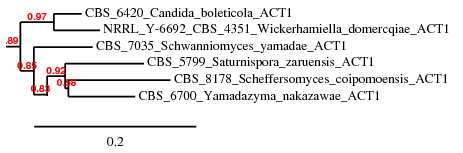
Using the publicly available database of [42], we assembled a dataset consisting of $n=6$ ACT1 gene DNA sequences ($m=540$ sites). We assumed the tree structure given in Figure 1 of Section A, and a Jukes-Cantor model of DNA evolution. We implemented our time-machine PMMH algorithm to infer $k$, $s_{1:k}$, and $\theta_{1:k+1}$ for cut-off parameter $g=4$ (see Supporting Information for further details). The prior on $k$ was a discrete uniform distribution on $\{0,1,2\}$, the prior on $s_{1:k}$ was uniform on $k$-subsets of $[m{-}1]$, and each substitution rate had a gamma prior with shape $=1$, scale $=0.3$.

We ran the algorithm for 10,589 iterations ($23$ days) on a Linux workstation that used twelve Intel Xeon E5-1650 3.20 GHz CPUs. We monitored convergence via autocorrelation and trace plots (Figure 3). We also monitored convergence of each model individually using the diagnostic in [43]; that is, we obtained a Z-score for each model parameter per each value of $k$ to get a sense of the algorithm’s ability to fully explore the state space of each model (only some values are reported below). Figure 3 suggests good exploration of the state space of $k$, resulting in an estimated distribution: $0.17$ ($k=0$), $0.47$ ($k=1$), and $0.36$ ($k=2$).

From the 4,946 samples with $k=1$, we estimated a 95% highest posterior density interval of (194,199) (see also the histogram in Figure 4). The Z-score for $k$ was $-0.60$, suggesting that we were still some way off convergence (values close to $0$ imply convergence). For the rates $\theta_{1}$ (before the change-point) and $\theta_{2}$ (after the change-point), the Z-scores of $0.11$ and $0.23$, respectively, give stronger evidence for convergence (estimated densities of these parameters are shown in Figure 5).

References

- [1] Felsenstein, J. (1981). Evolutionary Trees from DNA Sequences: A Maximum Likelihood Approach. J. Mol. Evol., 17, 368–376.
- [2] Felsenstein, J. (2004). Inferring Phylogenies. Sinauer, Sunderland, MA.
- [3] Huelsenbeck, J. P. & Suchard, M. A. (2007). A nonparametric method for accommodating and testing across-site rate variation. System. Biol., 56, 975-987.
- [4] Huelsenbeck, J. P. & Hillis, D. M. (1993). Success of phylogenetic methods in the four taxon case. System. Biol., 42, 247-264.
- [5] Wakeley, J. (1994). Substitution-rate variation among sites and the estimation of transition bias. Mol. Biol. Evol., 11, 436-442.
- [6] Swofford, D.L., Olsen, G.J., Waddell, P. J., & Hillis, D.M. (1996). Phylogenetic Inference. In Molecular systematics, 2nd edition, chap. 5, pp. 407-514. Sinauer and Associates, Sunderland, Massachusetts.
- [7] Uzzell T & Corbin K.W. (1971). Fitting discrete probability distributions to evolutionary events. Science, 172, 1089-96.
- [8] Nei M, Chakraborty R, & Fuerst P. A. (1976). Infinite allele model with varying mutation rate. Proc. Natl. Acad. Sci., 73, 4164–4168.
- [9] Olsen, G. J. (1987). Earliest phylogenetic branchings: comparing rRNA-based evolutionary trees inferred with various techniques. Cold Spring Harbor Symp Quant. Biol., 52, 825-837.
- [10] Yang, Z. (1995). A space-time process model for the evolution of DNA sequences. Genetics, 139, 993–1005.
- [11] Felsenstein, J & Churchill, G. A. (1996) A Hidden Markov Model approach to variation of evolutionary rates among sites. Mol. Biol. Evol., 13, 93-104.
- [12] Yang, Z., Goldman, N. & Friday, A. (1994). Comparison for models for nucleotide substitution used in maximum likelihood phylogenetic estimation. Mol. Biol. Evol., 11, 316–324.
- [13] Siepel A & Haussler D. (2005). Phylogenetic hidden Markov models. In R. Nielsen, editor, Statistical Methods in Molecular Evolution, pp. 325-351, Springer, New York.
- [14] Yang, Z. (1993). Maximum likelihood estimation of phylogeny from DNA sequences when substitution rates differ over sites. Mol. Biol. Evol., 10, 1396–1401.
- [15] Suchard, M. A, Weiss, R. E., Dorman, K. S. & Sinsheimer, J. S. (2003). Inferring spatial phylogenetic variation along nucleotide sequences: a multiple change-point model. J. Amer. Statist. Ass., 98, 427-437.
- [16] Pagel, M., & Meade, A. (2004). A phylogenetic mixture model for detecting pattern-heterogeneity in gene sequence or character-state data. Syst. Biol., 53, 571–581.
- [17] Loza-Reyes, E., Hurn, M.A. & Robinson A. (2014). Classification of molecular sequence data using Bayesian phylogenetic mixture models. Comp. Statist. Data Anal., 75, 81-95.
- [18] Wu, C. H., Suchard, M. A., & Drummond, A. J. (2013). Bayesian selection of nucleotide substitution models and their site assignments. Mol. Biol. Evol., 3, 669–688.
- [19] Boffelli, D., McAuliffe, J., Ovcharenko, D., Lewis, K. D., Ovcharenko, I., et. al. (2003). Phylogenetic shadowing of primate sequences to find functional regions of the human genome. Science, 299, 1391–1394.
- [20] Gibbs, R. A., Weinstock, G. M., Metzker, M. L., Muzny, D. M., Sodergren, E. J., et. al. (2004). Genome sequence of the Brown Norway Rat yields insights into mammalian evolution. Nature, 428, 493–521.
- [21] Chinwalla, A. T., Cook, L. L., Delehaunty, K. D., Fewell, G. A., Fulton, L. A., et. al. (2002). Initial sequencing and comparative analysis of the mouse genome. Nature, 420, 520–562.
- [22] Siepel, A., Bejerano, G., Pedersen, J. S., Hinrichs, A. S., Hou, M., et. al. (2005). Evolutionarily conserved elements in vertebrate, insect, worm, and yeast genomes. Genome Res., 15(8),1034–1050.
- [23] Mossel, E. & Vigoda, E. (2006). Limitations of Markov Chain Monte Carlo Algorithms for Bayesian Inference of Phylogeny. Ann. Appl. Probab, 16, 2215–2234.
- [24] Bouchard-Côté, A., Sankararaman, S. & Jordan, M. I. (2012). Phylogenetic inference via sequential Monte Carlo. System. Biol.. 61, 579-593.
- [25] Green, P. J. (1995). Reversible jump Markov chain Monte Carlo computation and Bayesian model determination. Biometrika, 82, 711–732.
- [26] Jasra, A., De Iorio, M., & Chadeau-Hyam, M. (2011). The time machine: a simulation approach for stochastic trees. Proc. R. Soc. A, 467, 2350–2368.
- [27] Karigiannis, G. & Andrieu, C. (2013). Annealed Importance Sampling Reversible Jump MCMC Algorithms. J. Comp. Graph. Statist., 22, 623–648.
- [28] Andrieu, C., Doucet, A., & Holenstein, R. (2010). Particle Markov chain Monte Carlo methods. J. R. Statist. Soc. Ser. B, 72, 269–342.
- [29] Del Moral, P., Doucet, A., & Jasra, A. (2006). Sequential Monte Carlo samplers. J. R. Statist. Soc. Ser. B, 68, 411–436.
- [30] Ma, Y. (2008). Bayesian and MCMC methods for phylogenetic footprinting. PhD Thesis, Imperial College London.
- [31] Pearl, J. (1982). Reverend Bayes on inference engines: A distributed hierarchical approach. In: Proceedings of the Second National Conference on Artificial Intelligence. AAAI-82: Pittsburgh, PA. AAAI Press, Menlo Park, CA.
- [32] Del Moral, P. (2004). Feynman-Kac Formuale. Springer: New York.
- [33] Zhou, Y., Johansen, A. M. & Aston, J. A. D. (2013). Towards Automatic Model Comparison: An Adaptive Sequential Monte Carlo Approach. arXiv preprint.
- [34] Jasra, A., Kantas, N., & Persing, A. (2014). Bayesian inference for partially observed stopped processes. Stat. Comp., 24, 1-20.
- [35] Fearnhead, P. & Liu, Z. (2007). Online Inference for Multiple Changepoint Problems. J. R. Statist. Soc. Ser. B, 69, 589–605.
- [36] Marin, J.-M., Pudlo, P., Robert, C.P. & Ryder, R. (2012). Approximate Bayesian computational methods. Statist. Comp., 22, 1167–1180.
- [37] Marin, J. M., Pillai, N. S., Robert, C. P., & Rousseau, J. (2013). Relevant statistics for Bayesian model choice. J. R. Statist. Soc. Ser. B, DOI: 10.1111/rssb.12056.
- [38] Del Moral, P., Doucet, A., & Jasra, A. (2012). An adaptive sequential Monte Carlo method for approximate Bayesian computation. Statist. Comp., 22, 1009–1020.
- [39] Toni, T., Welch, D., Strelkowa, N., Ipsen, A., & Stumpf, M. P. H. (2009). Approximate Bayesian computation scheme for parameter inference and model selection in dynamical systems. J. R. Statist. Soc. Interface, 6, 187–202.
- [40] Kong, A., Liu, J. S., & Wong, W. H. (1994). Sequential imputations and Bayesian missing data problems. J. Amer. Statist. Assoc., 89, 278–288.
- [41] Liu, J. S. (1996). Metropolized independent sampling with comparison to rejection sampling and importance sampling. Statist. Comp., 6, 113–119.
- [42] Weiss, S., Samson, F., Navarro, D., & Casaregola, S. (2013). YeastIP: a database for identification and phylogeny of ascomycetous yeasts. FEMS Yeast Res., 13, 117–125. http://genome.jouy.inra.fr/yeastip/
- [43] Geweke, J. (1992). Evaluating the accuracy of sampling-based approaches to calculating posterior moments. In Bayesian Statistics 4 (eds. Bernardo, J. M., Berger, J. O., Dawid, A. P., & Smith, A. F. M.). Clarendon Press, Oxford, UK.
- [44] Tavare, S., Balding, D. J., Griffiths, R. C., & Donnelly, P. (1997). Inferring coalescence times from DNA sequence data. Genetics, 145, 505–518.
- [45] Lopes, J. S., Balding, D., & Beaumont, M. A. (2009). PopABC: a program to infer historical demographic parameters. Bioinformatics, 25, 2747–2749.
- [46] Guennebaud, G., Jacob, B., et al. (2010). Eigen v3. http://eigen.tuxfamily.org.
Appendix A Figures
Real Data Case: Phylogeny of a subset of the Saccharomycotina subphylum
Sim. Data base dataset: Variability of for versus
Real Data Case: Autocorrelation and trace plot of sampled
Real Data Case: Histogram of sampled given
Real Data Case: Kernel density plots of sampled substitution rates given
Appendix B Tables