Simulated Magnetic Flows in the Solar Photosphere

Advances in instrumentation often lead to the discovery of new phenomena in the solar atmosphere. Thus, Borrero et al. (2010) found a large number of strongly blue-shifted Stokes V profiles in observations recorded by the Imaging Magnetograph eXperiment (Martínez Pillet et al., 2011a, IMaX,) on board Sunrise balloon-borne solar observatory (Barthol et al., 2011; Solanki et al., 2010; Berkefeld et al., 2011). By assuming hG vertical field and after taking the IMaX spectral resolution into account, Borrero et al. (2012) concluded that supersonic velocities are needed to produce such signatures at a wavelength shift of $\Delta\lambda=+227$ mÅ from the Fe I $525.02$ nm nominal line center. Since these features appear mostly above granules and thus are related to upflows, it is expected that the signal actually comes from the blueshifted neighbouring Fe I $525.06$ nm line.

Counterparts of these events were later found in Hinode/SP (Lites et al., 2001; Kosugi et al., 2007) data. Martínez Pillet et al. (2011b) assumed that Fe I $525.02$ nm and Fe I $630.25$ nm lines are similar and equally sensitive to all atmospheric parameters and identified signals that correspond to the same Doppler velocities. The difference with respect to IMaX results is that, while IMaX found $70$% of cases to be associated with upflows, in Hinode data blue-shifted and red-shifted profiles were equally present. On the other hand, both datasets, as well as the detailed study by Quintero Noda et al. (2013), showed that the events coincide with the appearance of linear polarization in the regions where the sign of the line-of-sight field was mixed. Based on these characteristics, both groups of authors concluded that reconnection of the emerging with pre-existing field could be the cause of these magnetic flows. This is supported by Borrero et al. (2013) who found a reversal in the polarity of the magnetic field along the line-of-sight, accompanied by an enhancement in the temperature and supersonic line-of-sight velocities.

We explore this scenario by using numerical 3D radiation MHD simulations of an emerging magnetic flux sheet in the presence of magnetic flux concentrations. We compute spectral line profiles in the simulated snapshots to simulate the IMaX or Hinode observations and compare the results to the observed signatures.

We consider two runs produced with the MURaM code (Vögler et al., 2005). The setup is essentially the same as in Cameron et al. (2011) with a checkerboard-like $2\times 2$ pattern of initial magnetic polarity, vertical magnetic field boundary condition at the upper boundary which is transparent for upflows and non-grey radiative transfer included. The computational domain of $6\times 6\times 1.68$ Mm was chosen with some $700$ km above $\tau_{500}=1$ and the resolution of $10$ and $14$ km in horizontal and vertical directions, respectively. Both ambipolar diffusion and the Hall current are included in the induction equation. These terms are expected to be important in the photosphere for dynamics at very small scales, especially in regions where the magnetic field gradients are large (Cheung & Cameron, 2012). At the current resolution (10 km in the horizontal directions) the effects on the dynamics of quiet-Sun features are relatively weak (Cheung & Cameron, 2012). A study of the full effects of the ambipolar and Hall effects is an interesting topic for future studies at higher spatial resolution.

Both runs start from the same snapshot of non-magnetic convection, to which a purely vertical magnetic field of positive and negative polarity was added. This initial field is arranged in a $2\times 2$ checkerboard pattern (Cameron et al., 2011, as in ), and has a height-independent strength of 200 G. The first run (from now on called the ’reference run’), was allowed to evolve freely from this initial condition, simulating the decay of the magnetic field in a mixed polarity region. For the second run we introduced a horizontal flux sheet $300$ km below mean optical depth unity, in order to simulate the scenario explained in the introduction. The field strength is set to vary across the cross section as a Gaussian with a FWHM of $110$ km with a maximum value of $1$ kG. We call this run - the ’emergence run’. In what follows all times are given with respect to the time at which the flux sheet was introduced in the second run.

Figure 1 shows a vertical cut through the initial snapshot (with the imposed sheet of horizontal flux) and the snapshot 188 s later. In the upper panel, the sheet is unmodulated, in its initial position. The field strength of $1$ kG at the center of the sheet gradually decrease to $0$ G at the edges. The added field was directed in the +X axis, i.e. aligned with the planes shown in this figure. At t$=188$ s most of the flux in this sheet has emerged. At this time, high-temperature structures are visible in locations where the emerging flux is reconnecting with the pre-existing magnetic field (green features in upper part of the simulation domain). We stress that it is not our aim to follow the detailed emergence and evolution of individual loops or the sheet in general. Rather, we are interested in the interaction of emerging flux with pre-exiting field in the solar photosphere. The number of such interactions is maximized with the initial magnetic configuration chosen here. Additionally, the time needed for the field to emerge is minimized.

To explore the observational signatures of these interactions, we synthesized the Sunrise/IMaX and Hinode/SP observables with the radiative transfer code SPINOR (Frutiger et al., 2000), based on the STOPRO routines (Solanki, 1987). The Fe abundance used for the synthesis is taken from Thevenin (1989) and the values of the oscillator strengths from the VALD database (Piskunov et al., 1995). For simulated IMaX data we synthesized the Fe I $525.02$ nm line, the Fe I $525.06$ nm line and the Co I $525.0$ nm line, which were then smeared with the IMaX spectral PSF. To simulate the effect of the phase diversity reconstruction technique with which the data were reconstructed that Borrero et al. (2010) used, we applied a low-pass filter that removes all spatial frequencies higher than $5.5$ arcsec^-1. We also took into account the stray-light which has been estimated empirically based on data recorded at the limb (Feller et al., in preparation). A noise of $3\cdot 10^{-3}$ I_c was added.

The Hinode/SP lines Fe I $630.15$ and $630.25$ nm were also computed. They were broadened with the Hinode/SP spectral PSF, as well as with a realistic spatial PSF (Danilovic et al., 2008). Finally, random noise of $8\cdot 10^{-4}$ I_c was added.

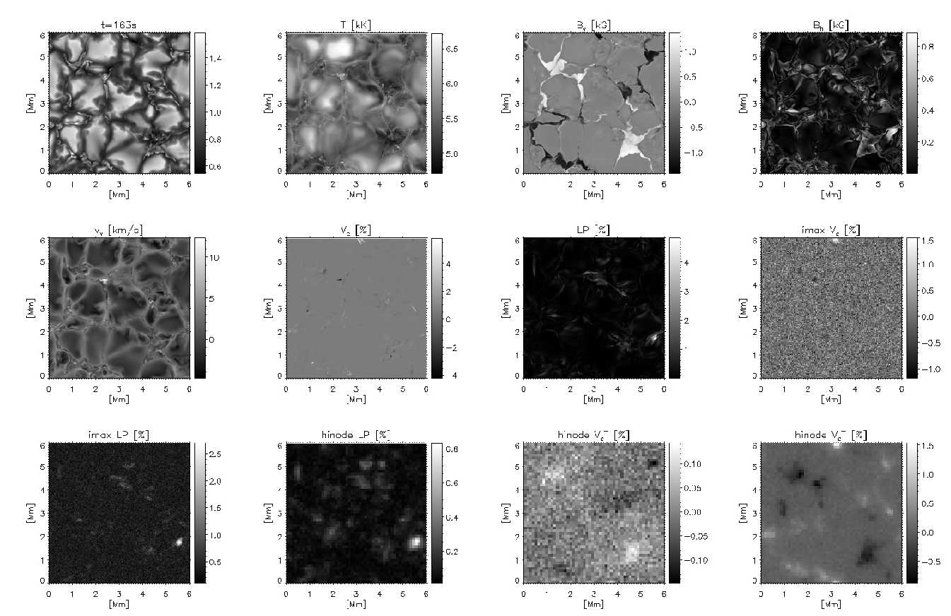
The simulation without the imposed horizontal flux sheet is similar to that studied by Danilovic et al. (2010). The main dynamical activity is the cancellation of flux between the opposite polarity magnetic elements. High velocities only occur in a few locations where several granules meet and magnetic field intensification takes place. Since the addition of the horizontal flux sheet leads to a substantial increase in the number of high velocity events, we will concentrate mainly on the ’emergence run’. Figure 2 shows various plasma properties on the $<\tau_{500}>=1$ plane from this simulation at t$=156$ s.¹¹ 1 Movies covering the $20$ minute period of both runs are available as on-line material. They combine all the maps shown in Figures 2, 3 and 4.

The flux sheet is significantly corrugated by the convective flows already $30$ s after the start. At around $90$ s, the first horizontal field crosses the $<\tau_{500}>=1$ plane. Then at $156$ s the whole simulation domain at that level is covered with horizontal magnetic field structures. Although the field strength was initially uniform in the horizontal direction, the loops are highly structured now. Fine structures in magnetic field are reflected in the fine structures in the intensity. The vertical field map shows footpoints of $\Omega$ loops as they sweep from the centres of granules towards their edges, at the same time increasing in strength as the material drains.

As the field emerges strong upflows appear at the +X edge of the pre-existing magnetic elements with negative polarity and on the -X edge of positive magnetic elements. These are locations at which the emerging field has the opposite polarity to the pre-existing field. An examination of the magnetic field lines shows that the high velocities correspond to U loops which are formed due to reconnection below the surface and are accelerated outwards by magnetic tension as they cross the photosphere. This outward acceleration leads to upflows and corresponding blue-shifts of spectral lines. In some cases the reconnection occurs at optical depth unity where strong magnetic concentrations are pushed together by the granular flow occurs. Reconnection jets with both upflows and downflows are then present.²² 2 An example of such processes can clearly be seen in the accompanying movie around $t=406$ s at $[2.5,4.5]$ Mm. Similar jets have previously been studied in more idealized simulations at different spatial scales (Takeuchi & Shibata, 2001; Isobe et al., 2008; Kigure et al., 2010).

On the other side of the flux concentrations (the -X edge of features with negative polarity and +X side of positive polarity features), the emerging flux leads not to a cancellation but to an enhancement of the field. This is consistent with the fact that the sheet of horizontal flux has zero net vertical flux. This enhancement of the magnetic field can initiate a ’collapse’ of the field (old and new) to kilo-gauss strengths. This process is aided in some cases by the draining of material down the field lines and produces strong negative vertical velocities, and consequently strong red-shifted features.³³ 3 An examples of such processes can clearly be seen in the accompanying movie around $t=375$ s at $[2.3,2.8]$ Mm.

Recent SUNRISE/IMaX observations revealed many short-lived events during which highly shifted circular polarization signals are detected. Their apparent association with the appearance of linear polarization signal and the nearby opposite magnetic polarity suggest that these events might be produced by the reconnection of the emerging with the preexisting field. Here, we use realistic 3D MHD simulations to investigate the applicability of this scenario. We introduce a uniform horizontal field $\approx 300$ km below the solar surface into a mixed polarity run and search for counterparts to the observed signatures. We simulate SUNRISE/IMaX and Hinode/SP observables. The simulations show that events similar to the observations tend to appear much more often when emergence is taking place and only in the locations where the high line-of-sight velocities coincide with the strong longitudinal magnetic field. These simulated events qualitatively match the observations. The synthesized line profiles are very similar to the observed ones. However there are a few significant deferences. The simulated events are on average considerably smaller and weaker than observed. For the mean lifetime and size of these events we obtain $57.4$ s and $7.6$ pixels, respectively, instead of $81.3$ s and $15.5$ pixels as found by Borrero et al. (2010) in the observations. Also, the huge majority of them appears in intergranular lanes and are associated with downflows, in contrast to observations. We believe that the size limit introduced by Borrero et al. (2010) removed most of these events. As a result, their analyses included only the cases that appear above granule. We find a few of these in our simulations. They are produced at the moment when the newly emerging flux appears at the surface. At these locations both, magnetic field and velocity drop rapidly with height. We find no change of polarity along the line of sight, as suggested by Borrero et al. (2013). Besides, our simulation give none of the height profiles presented in that paper. In the simulations, reconnection happens in the intergranular lanes where magnetic features of opposite polarity come into contact. Depending on the gradient of magnetic field, the temperature height profile can show a bump corresponding to an increase of $\approx 1000$ K. As a result, a shift in the formation height of the synthesized Fe I lines is produced. Because of this, lines usually miss to reveal dramatic events or show only associated downflows which take place below the temperature bump i.e. the reconnection site.

Why couldn’t we produce more of the observed-like examples? Having in mind that these features appear rather seldom, only few over 55${}^{\prime\prime}\times$55^′′ (Martínez Pillet et al., 2011b), this might not be so surprising. Thus, simulations that cover larger field of view and extend deeper in the convention zone are needed. We expect that such simulations will result in more realistic emergence events and wider spectra of magnetic field configurations that are not imposed by initial and boundary conditions as in our case.

Two movies for both the ’reference’ and the ’emergence’ runs are attached to the paper. Figures 9 and 10 show the styles from the movies.

References

- Barthol et al. (2011) Barthol, P., Gandorfer, A., Solanki, S. K., et al. 2011, Sol. Phys., 268, 1
- Berkefeld et al. (2011) Berkefeld, T., Schmidt, W., Soltau, D., et al. 2011, Sol. Phys., 268, 103
- Borrero et al. (2013) Borrero, J. M., Martínez Pillet, V., Schmidt, W., et al. 2013, ApJ, 768, 69
- Borrero et al. (2012) Borrero, J. M., Pillet, V. M., Schlichenmaier, R., et al. 2012, ASP Conference series, Vol 455, Edited by Luis R. Bellot Rubio, Fabio Reale, and Mats Carlsson. San Francisco: Astronomical Society of the Pacific, 2012, p.155
- Borrero et al. (2010) Borrero, J. M., Martínez-Pillet, V., Schlichenmaier, R., et al. 2010, ApJ, 723, L144
- Cameron et al. (2011) Cameron, R., Vögler, A., & Schüssler, M. 2011, A&A, 533, A86
- Cheung & Cameron (2012) Cheung, M. C. M., & Cameron, R. H. 2012, ApJ, 750, 6
- Danilovic et al. (2008) Danilovic, S., Gandorfer, A., Lagg, A., et al. 2008, A&A, 484, L17
- Danilovic et al. (2010) Danilovic, S., Schüssler, M., & Solanki, S. K. 2010, A&A, 509, A76
- Frutiger et al. (2000) Frutiger, C., Solanki, S. K., Fligge, M., & Bruls, J. H. M. J. 2000, A&A, 358, 1109
- Isobe et al. (2008) Isobe, H. and Proctor, M. R. E. and Weiss, N. O. 2008, ApJ, 679, L57
- Kigure et al. (2010) Kigure, H. and Takahashi, K. and Shibata, K. et al. 2010, PASJ, 62, 993
- Kosugi et al. (2007) Kosugi, T., et al. 2007, Sol. Phys., 243, 3
- Lites et al. (2001) Lites, B. W., Elmore, D. F., Streander, K. V., et al. 2001, Proc. SPIE, 4498, 73
- Martínez Pillet et al. (2011a) Martínez Pillet, V., Del Toro Iniesta, J. C., Álvarez-Herrero, A., et al. 2011, Sol. Phys., 268, 57
- Martínez Pillet et al. (2011b) Martínez Pillet, V., Del Toro Iniesta, J. C., & Quintero Noda, C. 2011, A&A, 530, A111
- Piskunov et al. (1995) Piskunov, N. E., Kupka, F., Ryabchikova, T. A., Weiss, W. W., & Jeffery, C. S. 1995, A&AS, 112, 525
- Quintero Noda et al. (2013) Quintero Noda, C., Martínez Pillet, V., Borrero, J. M., & Solanki, S. K. 2013, A&A, 558, A30
- Sainz Dalda et al. (2012) Sainz Dalda, A., Martínez-Sykora, J., Bellot Rubio, L., & Title, A. 2012, ApJ, 748, 38
- Solanki (1987) Solanki, S. K. 1987, PhD thesis No. 8309, ETH, Zürich
- Solanki et al. (2010) Solanki, S. K., Barthol, P., Danilovic, S., et al. 2010, ApJ, 723, L127
- Steiner (2000) Steiner, O. 2000, Sol. Phys., 196, 245
- Takeuchi & Shibata (2001) Takeuchi, A. & Shibata, K. 2001, ApJ, 546, L73
- Thevenin (1989) Thevenin, F. 1989, A&AS, 77, 137
- Vögler et al. (2005) Vögler, A., Shelyag, S., Schüssler, M., Cattaneo, F., Emonet, T., & Linde, T. 2005, A&A, 429, 335